
Abstract
Effect sizes typically vary among studies of the same intervention. In a random effects meta-analysis, this source of variation is taken into account, at least to some extent. However, when we have only one study, the heterogeneity remains hidden and unaccounted for. Treating the study-level effect as if it is the population-level effect leads to underestimation of the uncertainty. We propose an empirical Bayesian approach to address this problem. We start by estimating the distribution of the population-level effects and heterogeneity among 1635 meta-analyses from the Cochrane Database of Systematic Reviews. Using both synthetic data and cross-validation, we assess the consequences of using these estimated distributions as prior information for the analysis of single trials. We find that our Bayesian “meta-analyses of single studies” perform much better than naively assuming non-varying effects. The prior on the heterogeneity results in better quantification of the uncertainty. The prior on the treatment effect substantially reduces the mean squared error both for estimating the study-level and population-level effects. For the latter, this reduction is equivalent to doubling the sample size.
Introduction
It is common practice to interpret the observed treatment effect of a clinical trial as an estimate of an underlying true treatment effect. This is reasonable. We claim that it is also common to tacitly, perhaps even unconsciously, assume that this true effect is an immutable property of the treatment. Thus, one might speak of “the” effect of a particular treatment or intervention, and expect the same effect in another study about the same treatment. However, there are many good reasons to expect variation among the underlying effects from differences between study populations, application of the treatment and measurement protocols among other factors. There is also much empirical evidence of effect heterogeneity from random effects meta-analyses.1–3 Failure to take this into account when interpreting the results of a trial will lead to underestimation of the uncertainty about the treatment effect.
Recall that meta-analysis is a quantitative approach for combining inferences from multiple studies. Besides providing an estimate of the average or “population-level” effect of the treatment, together with some measure of uncertainty such as a standard error or confidence interval, a meta-analysis also provides an estimate of the variation of underlying effects of the individual studies. Understanding and quantifying heterogeneity is an important aspect of meta-analysis, as it can influence the interpretation of the overall results.
The Cochrane Database of Systematic Reviews (CDSR) is a globally respected collection of evidence-based healthcare information, comprising rigorous and comprehensive systematic reviews on diverse medical topics, with many of those reviews including meta-analyses. 4 The database is continuously updated, offering the latest evidence to inform clinical practice, policy decisions, and research priorities. It adheres to strict quality standards, undergoes peer review, and includes open-access summaries for wider accessibility.
We will assume the standard random effects meta-analysis model. That is, we assume the following two-part hierarchical (or multilevel) model for the


When we have only one study, we cannot separate the two error terms. Without additional assumptions, there is nothing more to do than estimate
Instead of assuming that
We compare the performance across the trials of the CDSR of our Bayesian approach to the naive approach of assuming that
Estimating the distributions of
and
Many of the systematic reviews in the CDSR are accompanied by meta-analyses. These data have been processed and made available by Schwab (2020). 8 Since the trials in the same meta-analysis are evaluating the same intervention, we can use the data from the CDSR to study how the effects of the same treatment vary across multiple studies.
We start by selecting trials with either a binary or numerical primary efficacy outcome; these comprise 97% of the trials in the CDSR. To make the effect sizes of the binary and numerical outcomes comparable, we quantify the treatment effect on the probit scale for all binary outcomes, and as the standardized mean difference (SMD) for all continuous outcomes. Next, we select all meta-analyses with at least 5 individual studies. Meta-analyses with fewer studies have little information about heterogeneity and discarding them reduces computation time. This leaves 18,368 unique trials from 1635 meta-analyses. We consider the following hierarchical model. For the


We want to estimate the distribution of the
To estimate the five parameters of our model (the mean, scale and degrees of freedom of the generalized
Estimated parameters of the
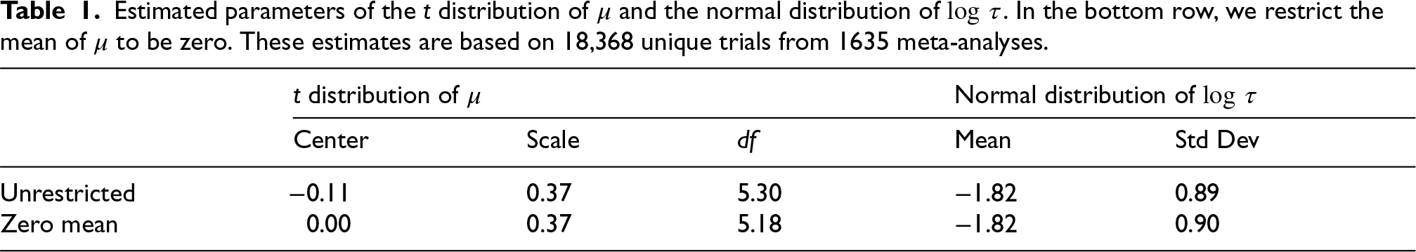
We can provide some context for these estimated distributions by recalling the tentative classification of effect sizes by Cohen according to which SMD values of 0.2–0.5 are considered small, 0.5–0.8 are considered medium, and >0.8 are considered large.9,10 The estimated
We also fit the model restricting the center of the distribution of effect sizes
We demonstrate our approach with a small example. Suppose that we have a single trial with a numerical outcome, with estimated SMD of
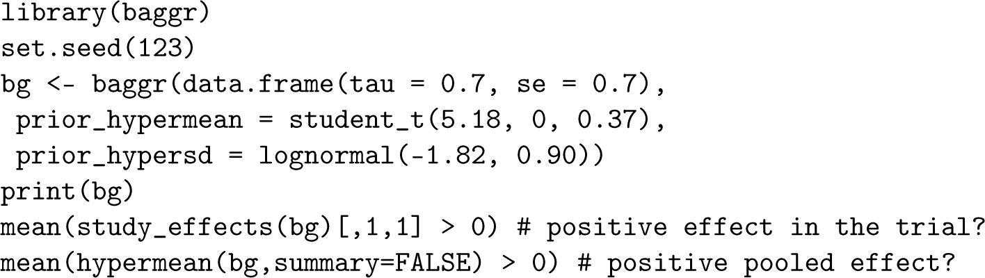
We can use the R package baggr to incorporate the prior information that is represented in Table 1. We first use a flat prior for the population-level effect

We find that the posterior distribution of the study-level effect (the true effect in the trial)
Next, we also incorporate information about the population-level effect
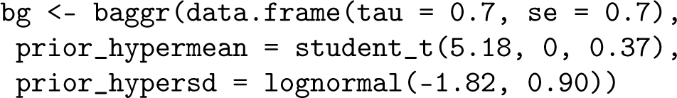
The zero-mean prior for
The probability of the correct sign
Next, we use baggr to perform all 18,368 meta-analyses with one trial and compute the posterior probabilities that the observed
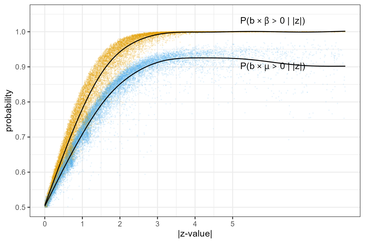
Conditional probabilities of
Building a synthetic CDSR
We construct a “synthetic” CDSR to evaluate the performance of our Bayesian approach and compare it to the naive approach of assuming that
Sample To induce dependence between the pairs Sample independent Sample
For
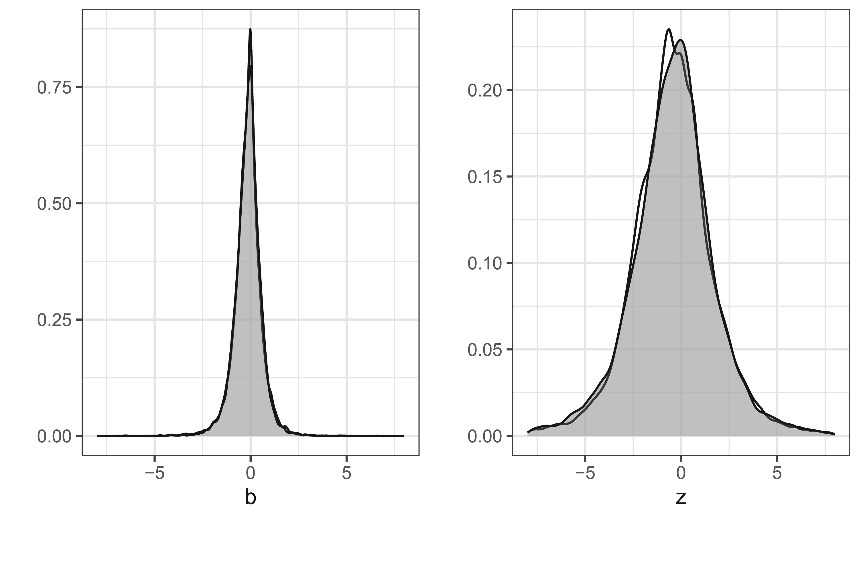
Observed and simulated distributions of 18,368 estimates and
Once again we use baggr to perform all meta-analyses with one trial in the simulated dataset to estimate
In Table 2, we show the root mean squared error (RMSE), bias of the magnitude, and coverage of these two estimators. To be precise, for the naive approach we compute


Performance of the unbiased estimators
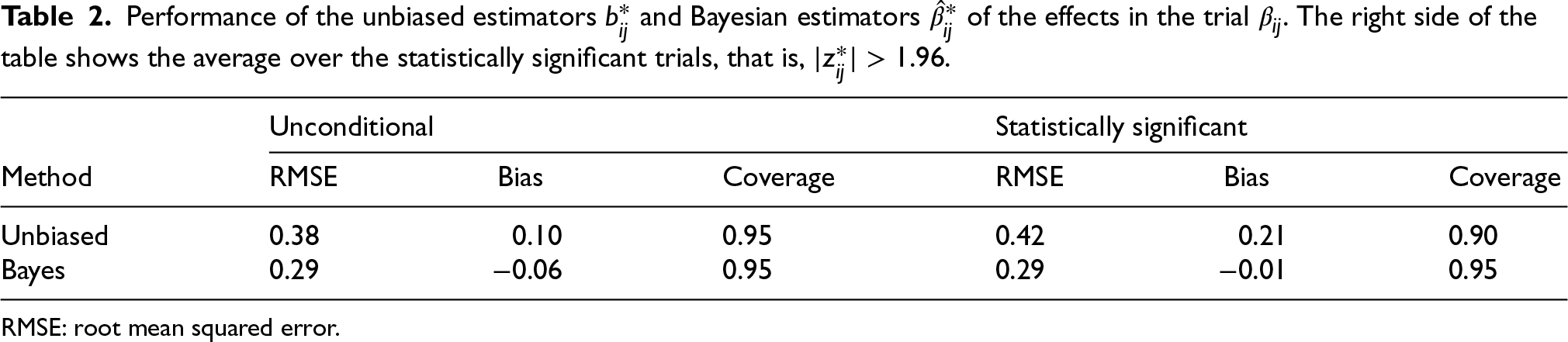
RMSE: root mean squared error.
We compute the analogous quantities for the Bayesian approach. The left side Table 2 displays the three performance measures for all trials and the right side by averaging only over the statistically significant trials with
Over all trials, the bias of the magnitude for the naive estimator is 0.1, which is due to Jensen’s inequality; recall that the absolute value is a convex function. As expected, the coverage of the usual confidence interval equals its nominal level. The right side of the table shows that selection on significance increases the upward bias of the magnitude to 0.21. This is sometimes called the “winner’s curse.” This bias also causes the mean squared error to increase. Moreover, the usual confidence interval no longer reaches nominal coverage.
When we turn to our Bayesian approach, we find that the RMSE is substantially reduced compared to the unbiased estimator: the MSE is reduced from
The reductions in the RMSE are due to the “shrinkage” that is induced by the zero-mean prior for
We also have two estimators for the population average effect
Performance of the unbiased estimators
and Bayesian estimators
of the population average effect
. The right side of the table shows the average over the statistically significant trials, that is,
.
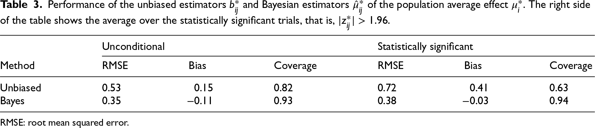
Performance of the unbiased estimators
RMSE: root mean squared error.
Essentially, the same observations apply to the results Table 3 as to those in Table 2. The reduction in the RMSE of the Bayesian estimator compared to the unbiased estimator is even more extreme. The MSE is reduced by more than a factor of 2 from
The coverage of the usual confidence interval is far below 95% both with and without conditioning on statistical significance. This is a direct result of not taking the heterogeneity into account. The coverage of the Bayesian uncertainty interval is close to nominal in both cases.
Tables 2 and 3 provide a broad overview of the performance of the naive and Bayesian estimators. We will now study the performance in some more detail both from the frequentist and Bayesian points of view. The frequentist point of view means that we condition on the true effects
We first consider the bias. The naive estimator
In the top left panel of Figure 3, we plot the estimation errors 
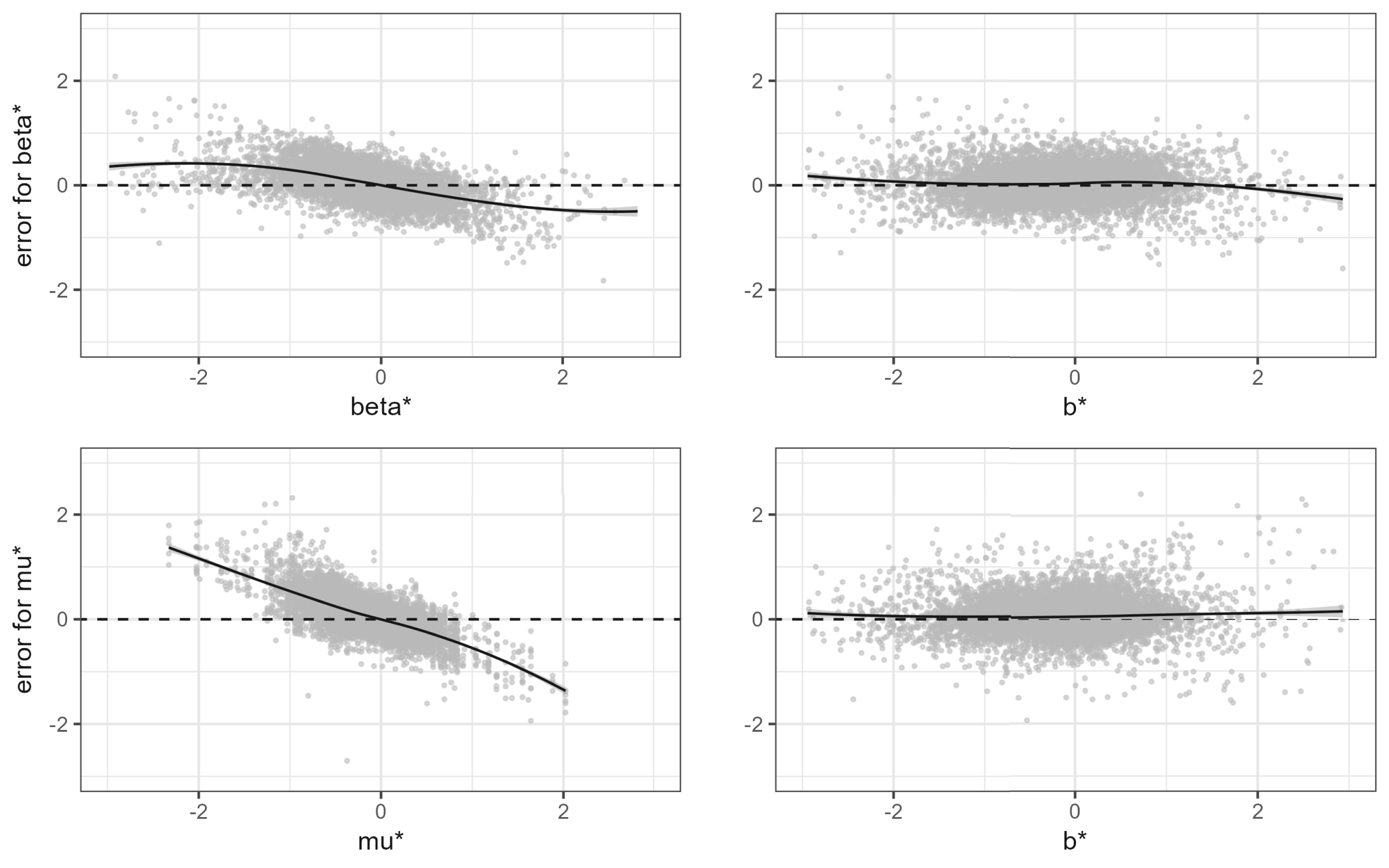
Bias of the proposed Bayesian estimators. The two top panels show
The two right panels paint a different picture. They show the bias in the Bayesian sense, that is, conditional on the observed effect. In this sense, the bias is negligible! The small bias that remains is due to our choice of a zero-mean prior while the average of the
Figure 4 shows the difference of the squared errors between the naive and Bayesian estimators. To be specific, in the top row we show these differences for estimating the 

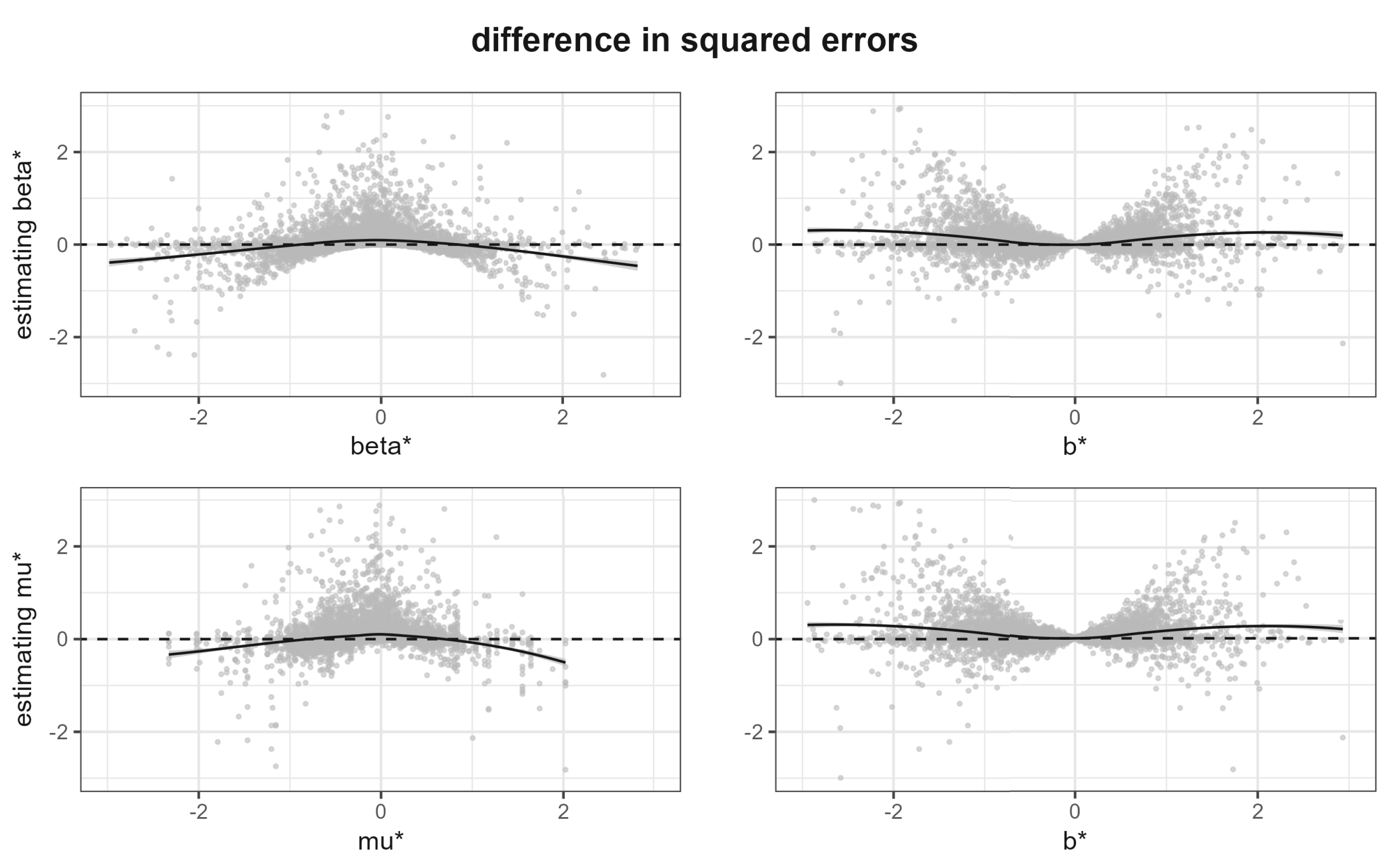
Difference in squared error of the naive and Bayesian estimators. Top row: difference in squared errors for
The two panels on the left side of Figure 4 show the frequentist perspective, where we condition on the true parameter values. We see that the Bayesian estimator performs better for small values of the parameter, while the naive estimator performs better for large values. The two panels on the right side of Figure 4 show the Bayesian perspective, where we condition on the observed
We have done our best to make sure that the synthetic CDSR closely resembles the true CDSR, so that the results of the previous sections also apply to the true CDSR. However, we cannot exclude the possibility that there are some systematic differences between the synthetic and true datasets which affect the relative performance of the Bayesian and naive estimators. However, we can conduct some additional checks that do not require synthetic CDSR.
First, since the estimates
Second, the first column in Table 3 provides an approximation of the difference in mean squared errors across the CDSR,


Despite
Consider three estimators 
If 
Using these results in applied research
Between-study variation of the treatment effect is often present in systematic reviews. Such heterogeneity may be due to differences in study populations, methodologies, or measurement techniques. In a random effects, meta-analysis the uncertainty due to between-study variation can be accounted for, but it remains hidden when we have only a single trial. In that case, without external information, there is no choice but to identify the within-study effect with the population-level effect. This leads to underestimation of the uncertainty about the population-level effect.
We propose a Bayesian approach, which we refer to as a “meta-analysis of a single trial,” where we estimate the distribution of treatment effects and heterogeneity across 1635 meta-analyses from the CDSR. Taking these estimated distributions as prior information provides a substantial improvement in performance both for estimating the effect in the trial (Table 2) and for estimating the population average effect among similar trials (Table 3). The Bayesian meta-analysis of a single trial can easily be done in R by using package baggr. 6
The Bayesian approach results in a large reduction of the RMSE across the trials of the CDSR compared to the usual unbiased estimator. This is to be expected for shrinkage estimation, and we have previously obtained similar results. 11 Here, we want to draw special attention to the substantial lack of coverage of the usual confidence interval for the population average effect; see Table 3. This is due to failure to account for the heterogeneity. In contrast, the coverage of the Bayesian uncertainty interval is equal to its nominal level.
Figure 1 shows that a single trial essentially never provides certainty about the sign of population average effect. This is a strong argument for the need for replication studies.
Since our prior distributions refer to the population of trials in the CDSR, our posterior statements can be interpreted in terms of random sampling from the CDSR. So, for example, we can say that if we randomly select a trial from the CDSR (or from the population of all the trials that could be in the CDSR) and we observe that the estimated treatment effect is
Now suppose we are interested in a particular trial where the estimated treatment effect is
We stress that we do not propose that our method should replace the usual estimate and its standard error. It is important that those are reported so that they may be combined with other information such as a meta-analysis at some later time.
About 75% of the meta-analyses in the CDSR have five or fewer studies. 4 When a meta-analysis consists of so few studies, it is clear that the heterogeneity cannot be estimated reliably without additional information. 1 Similarly as in the case of a single study that we outlined here, we should expect that doing a Bayesian meta-analysis with informative priors will improve inference. We intend to further evaluate the performance of this approach in a separate study.
The method we propose is especially well suited to decision making. Consider a decision maker choosing between interventions on the basis of a meta-analysis of a single or just a few studies. A model example would be the health technology assessment (HTA) process, which uses meta-analytic estimates to calculate cost-effectiveness. Both priors we propose play a role here. First, the prior on the mean effect induces shrinkage which helps avoid exaggeration of effect sizes. This leads to better rank ordering of treatments. Next, the prior on the heterogeneity improves the predictive distributions of effects, which can then be used by the decision maker to calculate fully Bayesian estimates of cost effectiveness. This matches the approach implemented in, for example, the UK by NICE (Dias et al. 12 ).
Bayesian meta-analysis
Statistical practice—Bayesian and otherwise—has incoherence with respect to the number of studies
When
As
When
With
When
Finally,
Reproducibility
The results in this article are fully reproducible with the R code provided in GitHub repository at github.com/wwiecek/singletrial. The data are publicly available at https://osf.io/xjv9g/. Below we provide the code snippet for calculating probability of positive effects in a trial or population; see the example in Section 2.2.
Supplemental Material
sj-pdf-1-smm-10.1177_09622802251380628 - Supplemental material for Meta-analysis with a single study
Supplemental material, sj-pdf-1-smm-10.1177_09622802251380628 for Meta-analysis with a single study by Erik van Zwet, Witold Wiȩcek and Andrew Gelman in Statistical Methods in Medical Research
Footnotes
Acknowledgements
We thank Simon Schwab and Rebecca Turner for their comments on an early draft of the article. Witold Wiȩcek received funding from FTX Future Fund regranting program to pursue research into meta-analytic methods. Andrew Gelman’s work was supported by ONR grant N000142212648.
Funding
The author(s) disclosed receipt of the following financial support for the research, authorship, and/or publication of this article: Witold Wiȩcek received funding from FTX Future Fund regranting program to pursue research into meta-analytic methods. Andrew Gelman’s work was supported by ONR grant N000142212648.
Declaration of conflicting interests
The author(s) declared no potential conflicts of interest with respect to the research, authorship, and/or publication of this article.
Supplemental material
Supplemental material for this article is available online.
References
Supplementary Material
Please find the following supplemental material available below.
For Open Access articles published under a Creative Commons License, all supplemental material carries the same license as the article it is associated with.
For non-Open Access articles published, all supplemental material carries a non-exclusive license, and permission requests for re-use of supplemental material or any part of supplemental material shall be sent directly to the copyright owner as specified in the copyright notice associated with the article.