
Abstract
Sequential trial emulation (STE) is an approach to estimating causal treatment effects by emulating a sequence of target trials from observational data. In STE, inverse probability weighting is commonly utilised to address time-varying confounding and/or dependent censoring. Then structural models for potential outcomes are applied to the weighted data to estimate treatment effects. For inference, the simple sandwich variance estimator is popular but conservative, while nonparametric bootstrap is computationally expensive, and a more efficient alternative, linearised estimating function (LEF) bootstrap, has not been adapted to STE. We evaluated the performance of various methods for constructing confidence intervals (CIs) of marginal risk differences in STE with survival outcomes by comparing the coverage of CIs based on nonparametric/LEF bootstrap, jackknife, and the sandwich variance estimator through simulations. LEF bootstrap CIs demonstrated better coverage than nonparametric bootstrap CIs and sandwich-variance-estimator-based CIs with small/moderate sample sizes, low event rates and low treatment prevalence, which were the motivating scenarios for STE. They were less affected by treatment group imbalance and faster to compute than nonparametric bootstrap CIs. With large sample sizes and medium/high event rates, the sandwich-variance-estimator-based CIs had the best coverage and were the fastest to compute. These findings offer guidance in constructing CIs in causal survival analysis using STE.
Keywords
Introduction
Target trial emulation with survival outcomes
Target trial emulation (TTE) has become a popular approach for causal inference using observational longitudinal data.1,2 The goal of TTE is to estimate and make inferences about causal treatment effects that are comparable to those that would be obtained from a target randomised controlled trial (RCT).1,3 TTE can be helpful when it is not possible to conduct this RCT because of time, budget and ethical constraints. Hernán and Robins (2016) have proposed a formal framework for TTE, 1 which highlights the need to specify the target trial’s protocol, that is, the protocol of the RCT that would have ideally been conducted, in order to guide the design and analysis of the emulated trial using data extracted from observational databases such as disease registries or electronic health records. The protocol should include the eligibility criteria, treatment strategies, assignment procedures, outcome(s) of interest, follow-up periods, causal contrast of interest and an analysis plan; see some step-by-step guides to TTE in Hernán et al., 4 Matthews et al., 5 and Maringe et al. 6
In TTE there are various sources of bias that must be addressed. Firstly, unlike in an RCT, non-random assignment of treatment at baseline must be accounted for when estimating the causal effect (intention-to-treat or per-protocol) of a treatment in an emulated trial. Secondly, similar to an RCT, it is necessary to account for censoring caused by loss to follow-up in an emulated trial. Thirdly, when the per-protocol effect is the causal effect of interest, it is also necessary to handle non-adherence to assigned treatments. To address these issues in TTE with survival outcomes, a useful approach is to fit a marginal structural Cox model (MSCM) using inverse probability weighting (IPW),7–13 after first artificially censoring the patients’ follow-up at the time of treatment non-adherence.14–16 Baseline confounders are included in this MSCM as covariates to adjust for the non-random treatment assignment at baseline using regression. The inverse probability weights are the product of two sets of time-varying weights: One to address selection bias from censoring due to loss to follow-up, and one to address selection bias from the artificial censoring due to treatment non-adherence. Counterfactual hazard ratios can be estimated from the fitted MSCM using weighted data. A modification of this approach is to discretise the survival time and replace the MSCM with a pooled logistic regression model.9,10 Provided that the probability of failure between the discrete times is small, this pooled logistic model well approximates the MSCM. 17
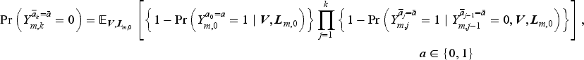
The counterfactual hazard ratio has been criticised as lacking a causal interpretation, and it has been proposed that other estimands be used instead, for example, the marginal risk difference (MRD).18–20 The MRD over time can be estimated by first using the counterfactual hazard ratio estimates from a marginal structural model (MSM) together with an estimate of the baseline hazard to predict the survival probabilities of the patients in the emulated trial under two scenarios: When all are treated and when none are treated. For each scenario, the predicted survival probabilities are averaged over all enrolled patients. The estimate of the MRD is then calculated as the difference between these two averages.16,20 This estimator is consistent, provided that the MSM for the survival outcome is correctly specified.
Constructing confidence intervals in sequential trial emulation
A potential problem when emulating a trial is that the number of treated and/or untreated patients eligible for inclusion in a trial that begins at any given time may be small. This can be addressed by sequential trial emulation (STE),14,21 which takes advantage of the fact that patients may meet the eligibility criteria for the target trial multiple times during their follow-up in an observational database. In STE, a sequence of target trials is emulated, each starting at a different time. The data from these sequential trials are pooled and analysed to produce an overall estimate of the treatment effect. 20 This approach was first proposed by Hernán et al. 14 and Gran et al. 21 as a simple way to improve the efficiency of treatment effect estimation relative to emulating a single trial. There have been several applications of STE; see Keogh et al. 20 for a list.
Despite the increasing popularity of TTE, there is a lack of research on different methods for constructing confidence intervals (CIs) of treatment effects in STE. The sandwich variance estimator, bootstrap or jackknife can be used to obtain a variance estimate of the parameter estimates in an MSM by accounting for correlations induced by the same patient being eligible for multiple trials. In causal survival analysis with IPW to adjust for baseline confounding of point treatments,22,23 the sandwich variance estimator of Lin and Wei 24 is frequently used. However, this estimator does not account for the uncertainty due to weight estimation, and can consequently overestimate the true variance.22,23 More complex sandwich variance estimators that account for this uncertainty are available. Shu et al. 23 proposed a variance estimator for the hazard ratio of a point treatment in an MSCM with IPW used for baseline confounding only. Enders et al. 25 developed a sandwich variance estimator for the hazard ratios in an MSCM when IPW is used to deal with treatment switching and censoring due to loss to follow-up. They found no substantial differences in the performance of the simple sandwich variance estimator and their sandwich variance estimator, and the latter performed comparatively poorly in scenarios with small sample sizes and many confounders. No off-the-shelf software has implemented the variance estimator by Enders et al. 25
Bootstrap has been recommended as an alternative to the sandwich variance estimator because it accounts for uncertainty in weight estimation. In the simple setting where IPW is used to estimate the effect of a point treatment on a survival outcome, Austin (2016) found that bootstrap CIs performed better than the sandwich-variance-estimator-based CIs when the sample size was moderate (1000). 22 In the setting with continuous and binary outcomes, Austin (2022) found that when sample sizes were small (250 or 500) to moderate (1000), bootstrap resulted in more accurate estimates of standard errors than sandwich variance estimators. However, bootstrap CIs did not achieve nominal coverage when the sample sizes were small to moderate and the treatment prevalence was either very low or very high. 26 Mao et al. (2018) observed similar results when constructing CIs of hazard ratios for a binary point treatment using IPW: With small (500) and moderate (1000) sample sizes and strong associations between confounders and treatment assignment, both the sandwich variance estimator and bootstrap resulted in under-coverage of CIs. 27 For the longitudinal setting with binary time-varying treatments, Seaman and Keogh (2023) found that with moderate (1000) sample sizes, bootstrap and the sandwich variance estimator both led to slightly under-coverage of CIs for hazard ratios in an MSCM but with no notable difference between the two methods. 28 With small (250, 500) sample sizes, the coverage of the CIs deteriorated, but bootstrap CIs had coverage closer to the nominal level than the sandwich-estimator-based CIs. 28
Jackknife resampling has been used in TTE to construct CIs of hazard ratio and risk difference (see Serdarevic et al. 29 and Virtanen et al. 30 for recent examples). Gran et al. (2010) also used jackknife to construct the CI of the hazard ratio of a binary treatment in the STE setting because in their analysis bootstrap led to non-convergence problems due to the large number of covariates used. 21 Jackknife could be advantageous when the sample size is small because it is computationally faster than bootstrap and it is less likely to lead to non-convergence problems since only one patient’s data are left out in each jackknife sample.
The works mentioned above all focussed on variance estimation and CIs for counterfactual hazard ratios, which are often chosen as the estimand in the literature of TTE with survival outcomes.14,31 While these works were not researched specifically for TTE with survival outcomes, they could be easily applied to such a setting. However, in the more complex setting of STE, less attention appears to be paid to the development and evaluation of CI construction methods. There is a lack of research on comparing the nonparametric bootstrap and the sandwich variance estimator for constructing CIs of the MRD in various settings of STE. It is also desirable to develop computationally more efficient CI methods than nonparametric bootstrap.
The contribution of this article
To fill this gap, we carry out an extensive simulation study to compare different methods for constructing a CI of the MRD in STE with a survival outcome. The first method uses the sandwich variance estimator that ignores the uncertainty caused by weight estimation. The second method is nonparametric bootstrap. This has the drawback of being computationally expensive. For this reason, the third method that we investigate is the computationally less intensive linearised estimating function (LEF) bootstrap. Hu and Kalbfleisch 32 first developed the estimating function bootstrap approach. In settings with cross-sectional/longitudinal survey data with design weights, Rao and Tausi 33 and Binder et al. 34 proposed the LEF bootstrap to improve computational efficiency and to avoid ill-conditioned matrices when fitting logistic models to bootstrap samples. We develop two forms of the LEF bootstrap for the STE setting. The fourth method is jackknife resampling. In our simulation study, we consider scenarios with varying sample sizes, treatment prevalence, outcome event rates, and strength of time-varying confounding. Our results provide some guidance to practitioners on which methods could perform better in different settings.
The article is organised as follows. In Section 2 we introduce the HIV Epidemiology Research Study (HERS) data as a motivating example and describe a protocol of STE based on the HERS data. Section 3 describes the notation, causal estimand, causal assumptions and MRD estimation procedure in STE. In Section 4, we describe the CI construction methods that we compare in this article, including our proposed LEF bootstrap CIs. Section 5 presents our simulation study. In Section 6, we apply STE to the HERS data. We conclude in Section 7 with a discussion.
HERS: A motivating example
The HERS included 1310 women with, or at high risk of, HIV infection at four sites (Baltimore, Detroit, New York, Providence) enrolled between 1993 and 1995 and followed up to 2000. 35 The HERS had 12 approximately six-monthly scheduled visits, where clinical, behavioural, and sociological outcomes and (self-reported) treatment were recorded.
Following Ko et al. 35 and Yiu and Su, 36 we aim to estimate the causal effect of (self-reported) Highly Active AntiRetroviral Treatment (HAART) on all-cause mortality among HIV-infected patients in the HERS cohort. Clinical and demographic variables related to treatment assignment and disease progression were available, including CD4 cell count, HIV viral load, self-reported HIV symptoms, race, and the site in which a patient was enrolled. Following Yiu and Su, 36 we treat visit 8 in 1996 as the baseline of the observational cohort, as HAART was more widely used and recorded in the HERS by then. There were 584 women assessed at visit 8. Time of death during follow-up was recorded exactly and there were 24 deaths in total. Some patients were also lost to follow-up, with 179 patients assessed at the last follow-up visit 12. Yiu and Su (2022) conducted their analysis with standard MSMs with IPW by defining the time-varying treatment as ordinal with 3 levels: ‘no treatment’, ‘antiretroviral therapy other than HAART’, and ‘HAART’. 36 In our analysis we consider a binary treatment: ‘HAART’ versus ‘no HAART’. A hypothetical RCT (the target trial) to estimate the per-protocol effect of HAART (vs. other or no treatment) on all-cause mortality could be emulated using the HERS data. The target trial protocol can be found in Table 14 of the Supplemental Materials.
As mentioned in Section 1, a practical problem for TTE is that if we only emulate a single trial, the number of patients who initiate (i.e. start to receive) the treatment at baseline and the number of outcome events among them could be small. In the HERS, only 76 patients initiated the HAART when baseline is defined as visit 8. By emulating a sequence of target trials and combining their analyses, more efficient estimates of treatment effects can be obtained. For example, an additional 62 women initiated HAART at visit 9 of the HERS, and so would be in the treatment arm of an emulated trial with baseline defined as visit 9.
In Section 6 we emulate 5 sequential trials from the HERS data labelled from 0 to 4 with sequential enrolment periods so that the trials start at visits 8, 9, 10, 11 and 12, respectively. The trial protocol, and more specifically the eligibility criteria, remain the same across all 5 trials, which in our example means that patients must have no prior use of HAART before the baseline of the trial. The study horizons differ: trial 0 has 4 follow-up assessments at visits 9–12; trial 1 has 3 follow-up assessments at visits 10–12; and so on. Trial 4 only has a baseline assessment at visit 12 and no further follow-up. This approach means that we can use data from patients who started receiving the HAART later in the HERS cohort. Table 1 presents tabulation of the HERS data prepared for STE, where we note that the total number of patients in the treatment arm is increased from 76 (in a single trial with baseline at visit 8) to 234 by using the STE approach. A patient can be eligible for multiple trials. For example, a patient who had not been receiving HAART at visits 8 and 9 but started to receive HAART from visit 10 will be eligible as a member of the control arm in trials 0 and 1, and as a member of the treatment arm in trial 2. Moreover, this patient’s follow-up in trials 0 and 1 will be artificially censored at visit 10. Figure 1 of the Supplemental Materials provides a schematic illustration of the STE approach.
Empirical coverage of the CIs in the scenarios with
Data tabulation of the HERS data prepared for a per-protocol analysis in STE.
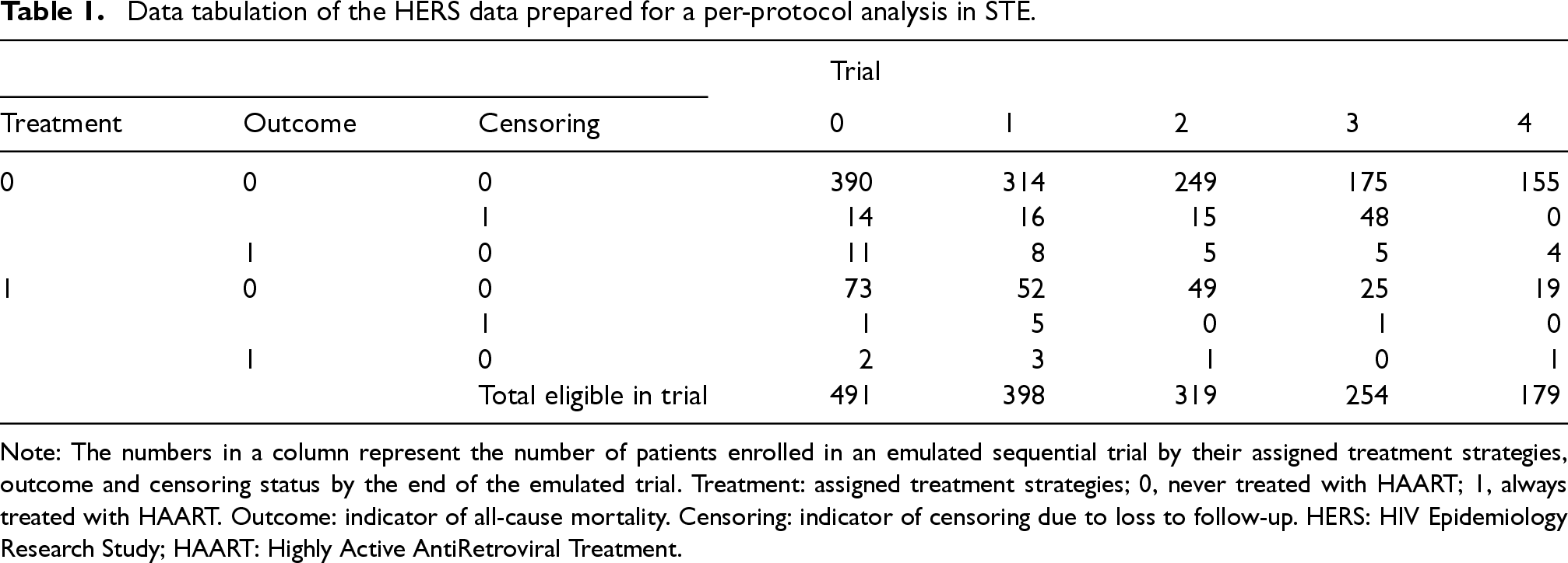
Note: The numbers in a column represent the number of patients enrolled in an emulated sequential trial by their assigned treatment strategies, outcome and censoring status by the end of the emulated trial. Treatment: assigned treatment strategies; 0, never treated with HAART; 1, always treated with HAART. Outcome: indicator of all-cause mortality. Censoring: indicator of censoring due to loss to follow-up. HERS: HIV Epidemiology Research Study; HAART: Highly Active AntiRetroviral Treatment.
Setting and notation
Consider an observational study in which
For a patient enrolled in trial
Causal estimand and assumptions
We define the per-protocol effect in trial 
Identification of (1) requires the following assumptions.
No Interference.
For
Consistency.
Positivity of treatment assignment, treatment adherence and censoring.
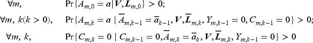
Sequentially ignorable treatment assignment.
Sequentially ignorable loss to follow up.
Equation (1) can be written equivalently as
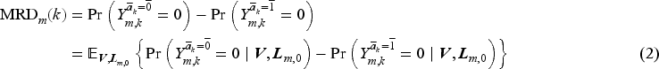
The counterfactual survival probabilities in (2) can be written in terms of counterfactual discrete-time hazards as follows:
We assume the following MSM in the form of a pooled logistic model with regression parameters 

Given the baseline covariates
To address artificial censoring due to treatment switching and censoring due to loss to follow-up, we calculate each patient’s stabilised inverse probability of treatment weight
We follow the method of Danaei et al., 31 who fitted logistic models to the treatment and censoring data from the original observational study to estimate the conditional probabilities used for calculating SIPTCWs. They used observed treatment and censoring data of each patient from the visits that correspond to the baselines of the eligible trials until the trial visits where the patient stopped adhering to the assigned treatments or the last trial visits. If patients were eligible for multiple trials, duplicates of the treatment and censoring data within patients were discarded.
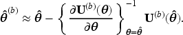
We pool the observed data from the
The MRD at trial visit 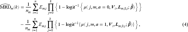
To summarise, the MRD in (2) is estimated by the following steps:
Estimate the SIPTCWs using data from the observational study. Expand the observational data by assigning patients to eligible sequential trials and artificially censor patients’ trial follow-up when they were no longer adhering to the treatment assigned at the baseline of each sequential trial. Estimate the MSM for the sequential trials using the expanded, artificially censored data with the estimated weights in Step 1. Create two datasets containing patients from a target population with their baseline covariates data, setting their treatment assignment to either treatment arm, and calculate the estimated counterfactual survival probabilities of each patient in each of these two datasets. Estimate the MRD by averaging the survival probabilities in each of the two datasets and taking the difference between these two averages, as is done in equation (4).
In this article, we use the
In this section, we describe the methods for constructing CIs of the MRD based on the simple sandwich variance estimator, nonparametric bootstrap, LEF bootstrap and jackknife resampling.
Sandwich variance estimator
The simple sandwich variance estimator accounts for the inverse probability weights and the correlation induced by patients being eligible to multiple trials.9,31 Specifically, for the pooled logistic regression model in (3), the simple sandwich variance estimator of 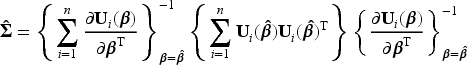
We follow the parametric bootstrap algorithm of Mandel (2013) to construct simulation-based CIs of the MRD as follows:
39
Obtain the parameter estimate Draw an i.i.d. sample For each vector Use the
This is currently the only CI method implemented in the
We use the non-Studentized pivot method
40
to construct CIs based on nonparametric bootstrap. Specifically, we follow the steps described below:
Draw For each bootstrap sample Define the lower and upper bounds of the 95% CI for the MRD at each trial visit
The main advantages of LEF bootstrap over nonparametric bootstrap are reduced computational time and non-convergence issues.32,34 In terms of computational time, unlike the nonparametric bootstrap, which involves fitting a regression model to each bootstrap sample, LEF bootstrap requires fitting this model only once to the original dataset. This can reduce computational time considerably, especially when iterative procedures are used to fit the model. In terms of non-convergence issues, Binder et al. (2004) found that when using nonparametric bootstrap for logistic regression it was possible to have several bootstrap samples for which the parameter estimation algorithm would not converge, due to ill-conditioned matrices that were not invertible.
34
For both reasons, LEF bootstrap may have advantages in our STE setting, where logistic regression models are used both for estimating the SIPTCWs and for fitting the MSM. We now explain how LEF bootstrap works in the general situation where the goal is to construct a CI for some function of a parameter vector
Let 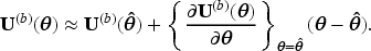

We propose the following two ways of using LEF bootstrap to construct CIs for the MRD.
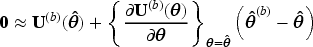
This approach applies Taylor linearisation only to the estimating function of the pooled logistic regression for the MSM in (3), with the SIPTCWs first being estimated from each bootstrap sample by fitting the corresponding logistic models to that bootstrap sample, as is done in nonparametric bootstrap. We shall use
Estimate Create Calculate approximate bootstrap parameter estimate For our case with a pooled logistic regression for MSM in (3), this formula can be written as
For the Construct the pivot CI using the
In the second approach, the Taylor linearisation is applied to the estimating functions of both the models for estimating SIPTCWs and the pooled logistic regression for the MSM (3). Approach 2 should be even more computationally efficient than Approach 1, because it avoids fitting the models for the SIPTCWs to each bootstrap sample. Moreover, Approach 2 could be useful when there are many covariates (relative to the sample size) in the models for the SIPTCWs, in which case ill-conditioned matrices could arise when fitting these models to some of the bootstrap samples.
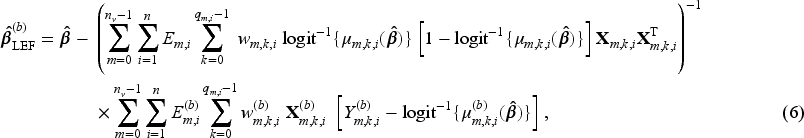
Because multiple models have to be fitted to obtain the SIPTCWs, we explain the steps for implementing the LEF bootstrap using the model for the denominator term of the stabilised inverse probability of treatment weights (IPTWs, see equation (1) of the Supplemental Materials) given
Let Fit the weighted pooled logistic model to the original dataset and obtain the point estimate Create Calculate the LEF bootstrap parameter estimates of the models for estimating SIPTCWs for each bootstrap sample according to (5). For example, the LEF bootstrap estimates Based on LEF bootstrap parameter estimates for the models for estimating SIPTCWs, calculate a new set of weights Construct the pivot CI using Steps (3)–(5) in Approach 1 in Section 4.3.1, replacing 
We use jackknife resampling to construct two types of jackknife-based CIs: (1) using a jackknife estimate of the MRD standard error,
41
and (2) using the jackknife variance estimator42,43 of
Approach 1: Wald-type CI using the jackknife estimate of the MRD standard error
We use the jackknife estimator of the standard error of the MRD estimate and a Normal approximation to obtain CIs as follows:
Obtain the parameter estimate For Obtain the jackknife standard error estimate Define the lower and upper bounds of the 95% CI for the MRD at trial visit

We use the jackknife variance estimator42,43 of Obtain the parameter estimate For Obtain the jackknife variance estimate Construct a 95% CI by repeating Steps (2)–(4) of Section 4.1 and replacing the sandwich variance matrix estimate

We conducted an extensive simulation study to compare the performance of CIs obtained using the sandwich variance estimator, nonparametric bootstrap, the proposed LEF bootstrap and jackknife methods. For simplicity, we assumed there was no loss to follow-up.
Study setup
Data generating mechanism
We used the algorithm described in Young and Tchetgen Tchetgen 37 to simulate data. This algorithm ensure that previous treatments affect time-varying variables (confounders) that are associated with both current treatment and hazard of the outcome event. The data generating mechanism is described in Table 2.
Summary of data generating mechanism of the simulation study.
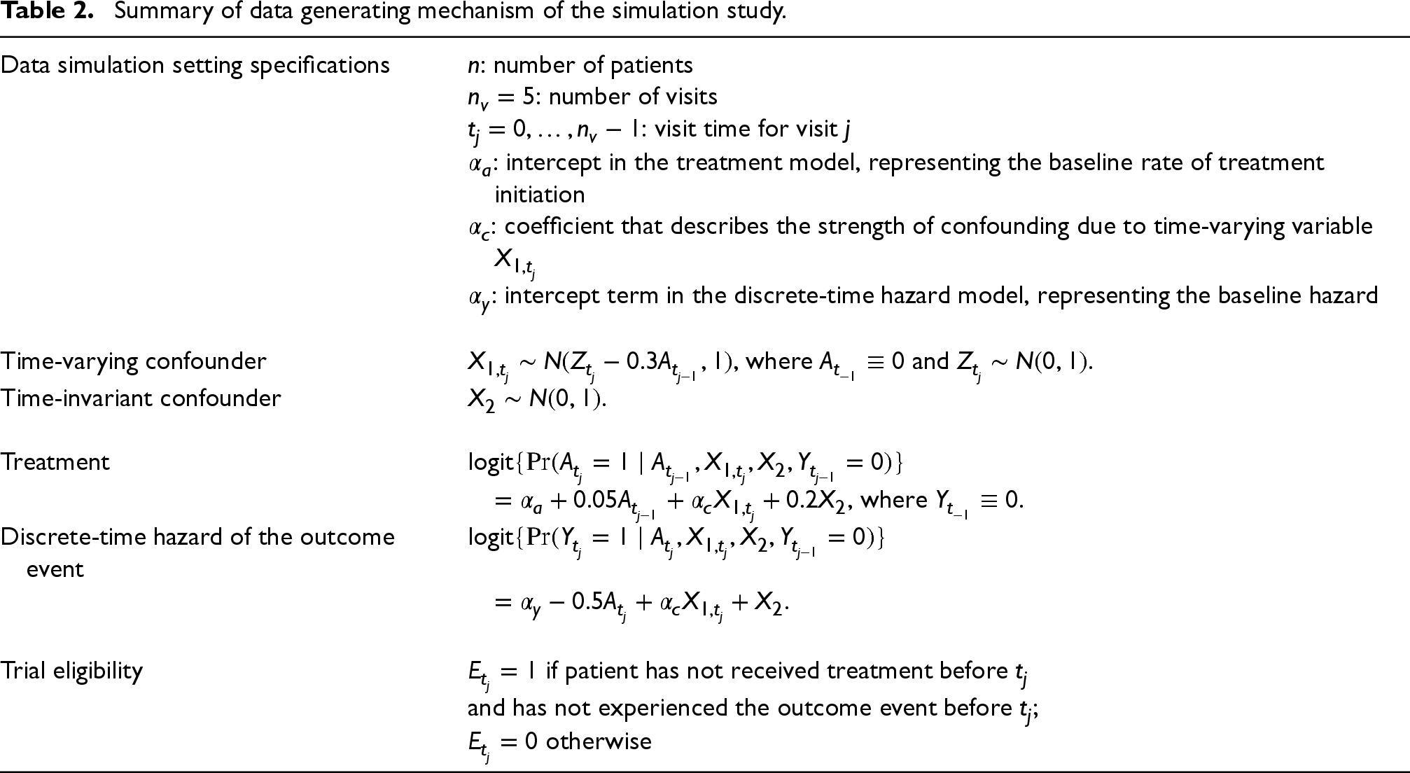
Summary of data generating mechanism of the simulation study.
We considered three settings with different outcome event rates, by setting the baseline hazards
Summary of the specifications for the 81 scenarios considered in the simulations.
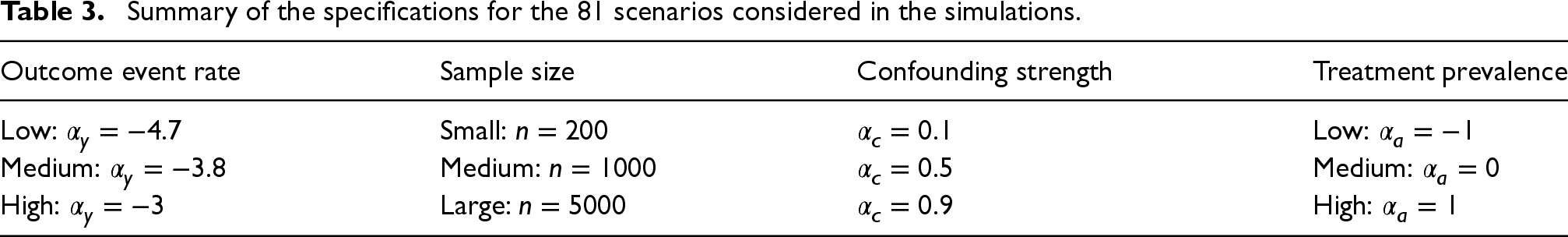
Summary of the specifications for the 81 scenarios considered in the simulations.
For each simulated dataset, we emulated 5 trials (
Correctly specified logistic regression models were fitted to the simulated data to estimate the denominator terms of the stabilised IPTWs in equation (1) of the Supplemental Materials, while the numerator terms were estimated by fitting an intercept-only logistic model stratified by treatments received at the immediately previous visit
Then the following weighted pooled logistic model was fitted to the artificially censored data in the five sequential trials to estimate the counterfactual discrete-time hazard:

We applied the methods for constructing 95% CIs of the MRD in Section 4 to each simulated dataset, where we set
True values of the MRDs for each simulation scenario were obtained by generating data for a very large randomized controlled trial, as proposed by Keogh et al.
20
The true marginal risks in trial 0 when all patients were always treated or all patients were never treated were approximated by Kaplan–Meier estimates from two extremely large datasets (
Additionally, for each simulation scenario, we fitted the same weight estimation models and MSM in Section 5.1.3 to multiple simulated datasets, each with 200,000 patients. We then averaged the resulting MRD estimates to compute ‘pseudo-true’ MRDs induced by the misspecified MSM. The absolute difference between the ‘pseudo-true’ MRDs and the corresponding Kaplan–Meier estimates of the true MRDs were all less than 0.001. More details about these ‘pseudo-true’ values are provided in Section 5.4 of the Supplemental Materials.
Performance measures
Empirical coverage of the CIs was calculated for each trial visit in each simulation scenario. This was done by dividing the number of times that a CI of the MRD contained the true MRD by 1000 minus the number of times there was an error in the CI construction. Such errors include issues with the sandwich variance estimation or jackknife variance estimation that led to non-positive definite variance matrices. We also considered bias-eliminated CI coverage to adjust for the impact of bias in the coverage results. 45 This involved calculating the proportion of the 1000 CIs that contained the sample mean of the 1000 MRD estimates for each scenario.
Morris et al.
45
state four potential reasons for CI under- or over-coverage when examining simulation results: (i) MRD estimation bias, (ii) the standard error estimates from a CI method underestimate the empirical standard deviation (SD) of the MRD estimator, (iii) the distribution of the MRD estimates is not normal and CIs have been constructed assuming normality, and (iv) the standard error estimates from a CI method are too variable. Therefore, for each simulation scenario, we calculated the empirical bias of the MRD estimates at each trial visit to check reason (i) for CI under-coverage. For each CI method, we calculated the SD of the MRD estimates (from resampling), denoted as
We recorded the number of times that each CI method encountered an error (a ‘construction failure’). We also calculated the Monte Carlo standard error of the empirical coverage (due to using a finite number of simulated datasets):
45

Finally, we reported the relative computation time that it took to construct CIs based on nonparametric bootstrap, LEF bootstrap and jackknife compared to CIs based on the sandwich variance estimator.
The simulations were conducted using
Results
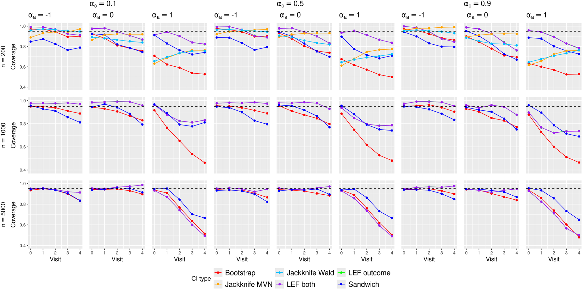
In this section, we focus on the discussion of the results in low event rate scenarios; results for medium and high event rate scenarios can be found in Section 5 of the Supplemental Materials. The reason for this focus is two-fold: (1) The HERS data example had low event rates; (2) the CI methods performed the worst in low event rate scenarios and yet we still observed interesting patterns for their relative performance, which were not drastically different from those in medium and high event rate scenarios.
Figure 1 shows the empirical coverage rates of the CIs when the event rate was low, using the true values by Kaplan–Meier estimates; see Figures 2 and 3 of the Supplemental Materials for results with medium and high event rates. Differences between these coverage rates and the corresponding bias-eliminated coverage rates were negligible (see Figures 4 to 6 of the Supplemental Materials). We also calculated the coverage rates using the ‘pseudo-true’ MRDs induced by the misspecified MSM. The differences between the coverage rates based on the ‘pseudo-true’ MRDs (Figures 7 to 9 of the Supplemental Materials) and those based on the true MRDs calculated using Kaplan–Meier estimates (Figure 1 of the main text and Figures 2 and 3 in the Supplemental Materials) were negligible. Thus we focus on the simulation results based on the true MRDs calculated using Kaplan–Meier estimates in the following discussions.
We will initially examine the bias of the MRD estimates, followed by the SE ratio results for the CI methods, to explain the under-coverage or over-coverage of the CIs and the relative performance of these CI methods in various simulation scenarios. Afterwards, we will discuss computation time for the CI methods. Results for Monte Carlo standard errors of the CI coverage estimates and CI construction failure rates can be found in Sections 5.7 and 5.8 of the Supplemental Materials. Since we observe very little difference in the performance of the two LEF bootstrap CI methods, we will refer to them as one when discussing the results. We refer to the CIs constructed using the sandwich variance estimator as ‘Sandwich CIs’, those using Approach 1 from jackknife resampling as ‘Jackknife Wald CIs’ and those using Approach 2 as ‘Jackknife Multivariate Normal (MVN) CIs’.
Empirical bias and its impact on CI coverage
Figure 2 presents the empirical biases of the MRD estimates.
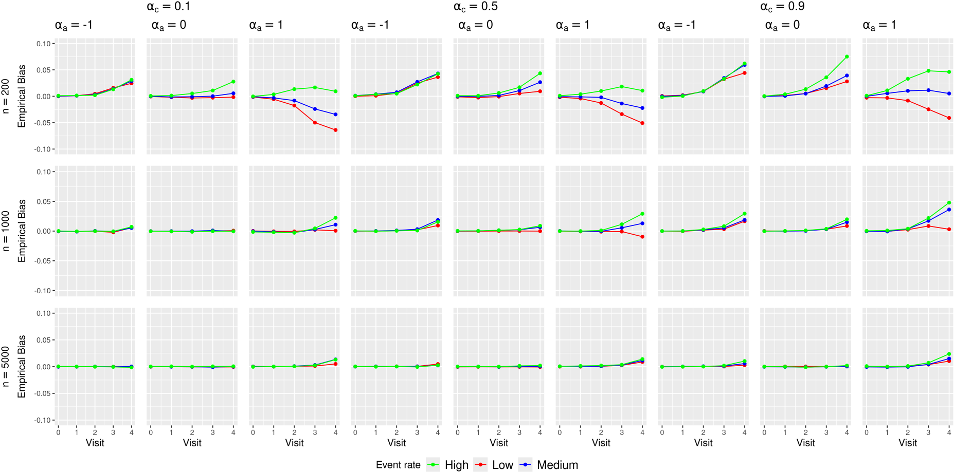
Empirical biases of the marginal risk difference (MRD) estimates in various simulation scenarios.
Minimal biases were observed at earlier visits (
The absolute biases in low or high treatment prevalence scenarios were larger than those in medium treatment prevalence scenarios. This likely stemmed from data sparsity issues at later trial visits that were aggravated by treatment arm imbalance caused by low or high treatment prevalence. Table 1 of the Supplemental Materials shows an example of this imbalance.
No clear patterns were observed for the impact of confounding strength and outcome event rate on the bias. The direction and magnitude of the bias appear to differ by the combinations of these scenarios.
These bias results explain the general trends of CI coverage in Figure 1. As the sample size increased, the CI coverage at earlier visits approached the nominal 95% level, which was not surprising given that all the methods rely on asymptotic approximations. The increasing absolute bias at later visits (
In scenarios with low treatment prevalence (
We note that the poor coverage in low or high treatment prevalence scenarios does not appear to originate from practical violations of the positivity assumption. Table 12 in Section 5.5 of the Supplemental Materials presents summary statistics of the estimated IPTWs stratified by assigned treatments from a large data set with
We observed minimal impact of confounding strength on CI coverage. Increasing the event rate improved the CI coverage for all methods most prominently in scenarios with larger sample size (
The empirical SD and the root-mean squared error (MSE) of the MRD estimates largely followed the patterns of the bias (see Figures 10 and 11 of the Supplemental Materials): scenarios with larger biases also exhibited larger SDs and MSEs.
Figures 3 and 4 present the summary statistics of the SE ratio,
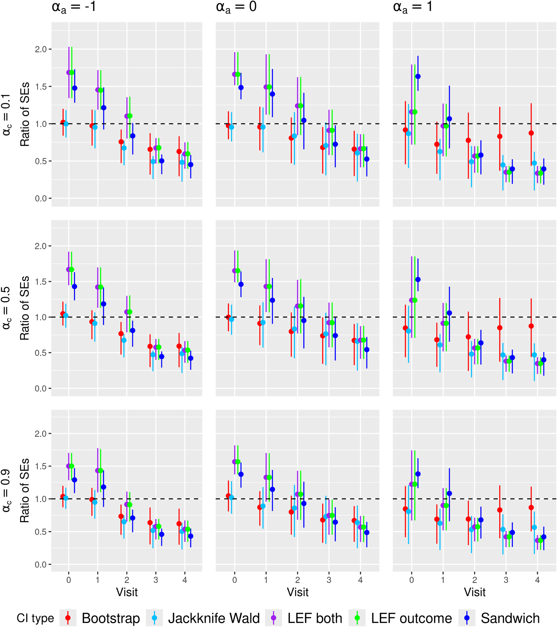
Ratio of the estimated standard error to empirical standard deviation of the MRD estimator (SE ratio) in
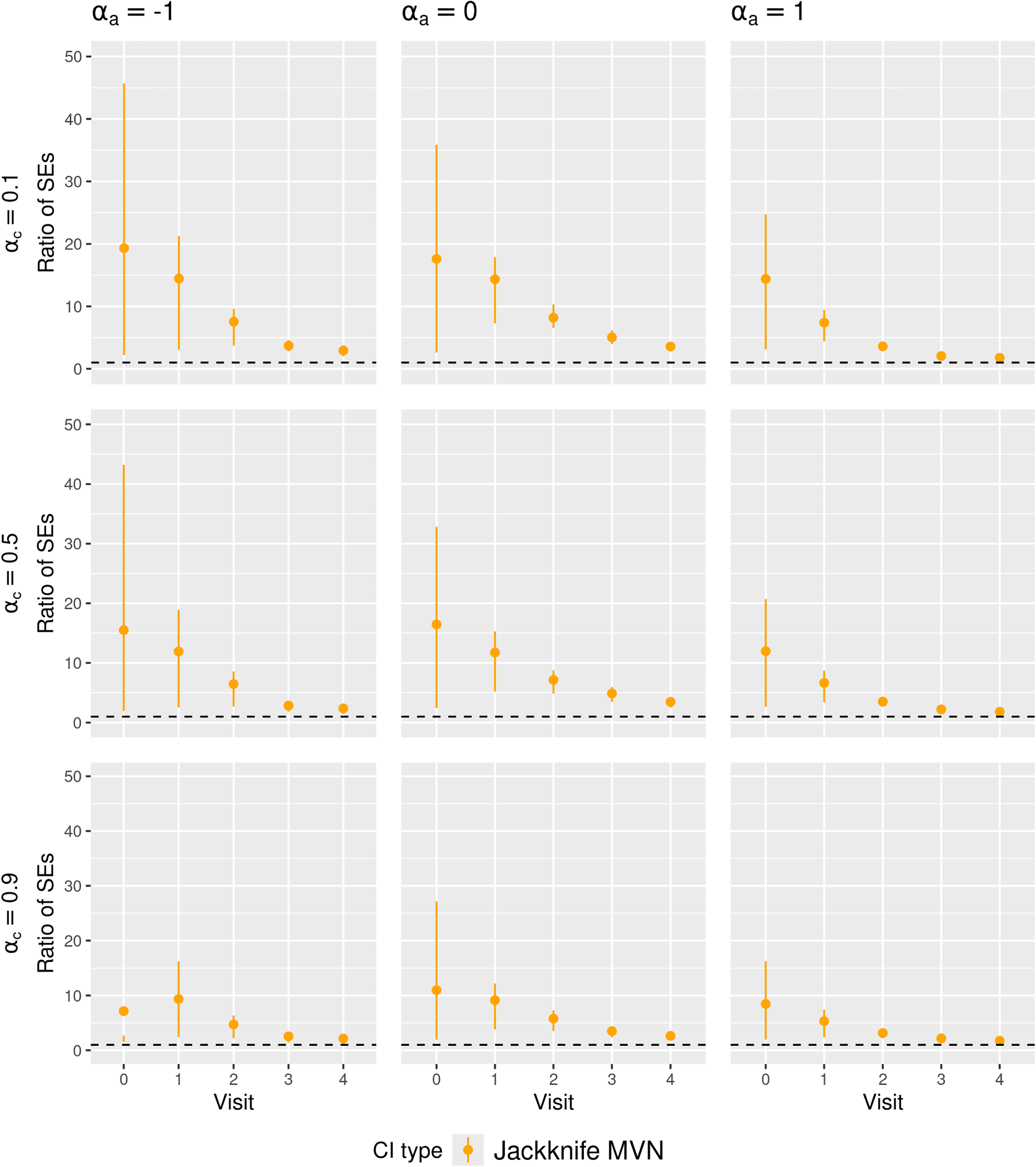
Ratio of the estimated standard error to empirical standard deviation of the MRD estimator (SE ratio) in
We found that the SE ratio results largely explained the differences in CI coverage of the various CI methods. The comparative performance of the CI methods in terms of coverage generally followed the patterns of the SE ratios: when the average SE ratios were above 1, we observed over-coverage; when the average SE ratios were about 1, we observed close to nominal coverage; when the average SE ratios were below 1, we observed under-coverage. Higher variability of the SE ratios also coincided with lower CI coverage. Notably, in scenarios with high event rate, large sample size, medium treatment prevalence and weak confounding, all CI methods achieved close-to-nominal coverage, which corresponded to all CI methods having SE ratios close to 1 on average and with low variability.
In Figure 3, the SE ratios for Jackknife Wald CIs were also lower than 1 at later visits, but in low and high treatment prevalence scenarios, they were less variable compared to those for nonparametric bootstrap CIs, which might partly explain the better coverage of Jackknife Wald CIs in these scenarios. However, in Figure 4, the SE ratios for Jackknife MVN CIs were much larger than 1 in all scenarios with small sample sizes, which may explain the over-coverage or closer-to-nominal coverage for Jackknife MVN CIs in some scenarios.
In Figure 3, the SE ratios for LEF bootstrap CIs and Sandwich CIs were larger than 1 at early visits (
With increased event rates, we observed that differences in CI coverage among the methods were primarily due to SE ratio variability. In most scenarios with medium/high event rates and medium/large sample sizes, the average SE ratios of Sandwich CI and LEF bootstrap CIs were very similar but the SE ratios of Sandwich CIs tended to be less variable, which might lead to their better coverage. With medium/large sample sizes, nonparametric bootstrap CIs and LEF bootstrap CIs had similar SE ratios, resulting in similar coverage, whereas with small sample sizes, the SE ratios of nonparametric bootstrap CIs tended to be much more variable than those for LEF bootstrap CIs particularly at later visits, leading to worse coverage.
We also observed close-to-nominal coverage for Jackknife Wald CIs in scenarios with small sample size, low treatment prevalence and medium/high outcome event rate, which could be explained by smaller variability in their SE ratios with increased event rates. In such scenarios, SE ratios of Jackknife Wald CIs were also closer to 1 for all visits, compared to the low event rate scenario. The SE ratios of Jackknife MVN CIs were still larger than 1 but became less variable. This is consistent with their slight over-coverage or close-to-nominal coverage in scenarios with small sample size, low/medium treatment prevalence and medium/high outcome event rates.
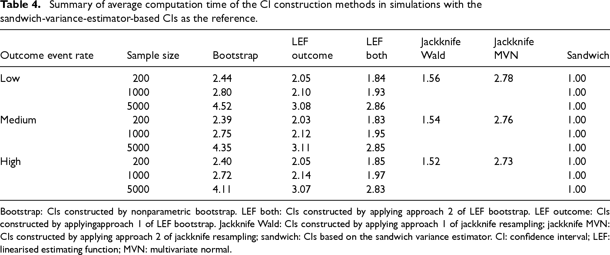
Table 4 summarises the average computation time (across 1000 simulated data sets and the scenarios of treatment prevalence and confounding strength) for constructing a CI of the MRD using each method, relative to the time for constructing Sandwich CI. On average, nonparametric bootstrap CIs took about 2.4–4.5 times longer to compute than Sandwich CIs. The computation time increased exponentially as sample sizes increased. LEF bootstrap CIs, using both Approaches 1 and 2, took about 1.8–3 times longer to compute compared to Sandwich CIs.
Summary of average computation time of the CI construction methods in simulations with the sandwich-variance-estimator-based CIs as the reference.
Summary of average computation time of the CI construction methods in simulations with the sandwich-variance-estimator-based CIs as the reference.
Bootstrap: CIs constructed by nonparametric bootstrap. LEF both: CIs constructed by applying approach 2 of LEF bootstrap. LEF outcome: CIs constructed by applyingapproach 1 of LEF bootstrap. Jackknife Wald: CIs constructed by applying approach 1 of jackknife resampling; jackknife MVN: CIs constructed by applying approach 2 of jackknife resampling; sandwich: CIs based on the sandwich variance estimator. CI: confidence interval; LEF: linearised estimating function; MVN: multivariate normal.
For small sample sizes (
The large gain in computational efficiency through LEF bootstrap is very much of interest; with large sample sizes (
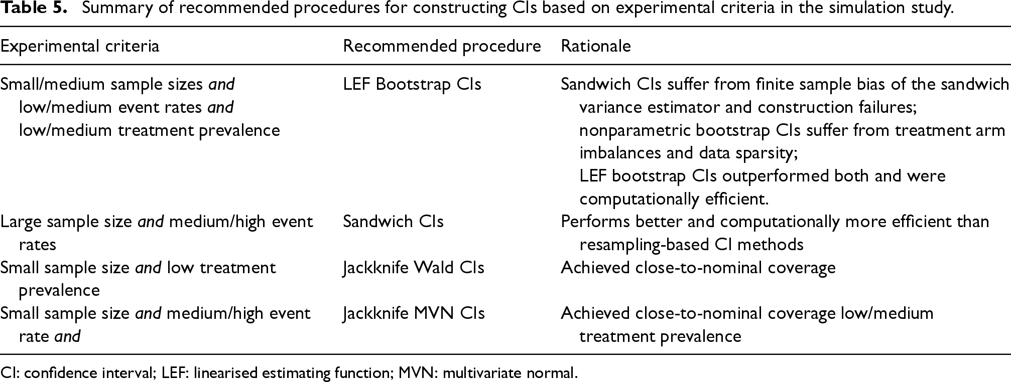
Our simulation results suggest that LEF bootstrap CIs provided better coverage compared to Sandwich CIs in scenarios with small/medium sample sizes, low/medium outcome event rates and low/medium treatment prevalence. This might be attributed to the finite sample bias of the sandwich variance estimator and high frequency of the construction failure of Sandwich CIs in such scenarios. The performance of nonparametric bootstrap CIs was considerably affected by treatment arm imbalance and data sparsity, particularly in scenarios with low event rates and small/medium sample sizes. In these scenarios, the LEF bootstrap method not only performed better but was also more computationally efficient than nonparametric bootstrap. While Jackknife Wald CIs achieved nominal coverage with small sample sizes and low treatment prevalence, their performance plummeted with medium/high treatment prevalence. With medium/high outcome event rates and low/medium treatment prevalence, Jackknife MVN CIs also achieved close-to-nominal coverage, possibly due to their overall conservativeness. Due to data sparsity and finite-sample bias, all methods performed poorly when treatment prevalence was high, and Jackknife MVN CIs faced numerous construction failures, making them impractical for use.
Since STE is particularly useful for data scenarios with small numbers of patients initiating treatments at any given time (low treatment prevalence) and with low event rates, LEF bootstrap offers a useful alternative to the sandwich variance estimator and the nonparametric bootstrap for CI construction, especially in small/medium sample sizes. Although Jackknife Wald CIs and Jackknife MVN CIs also provided good coverage in some scenarios, they become computationally inefficient as the number of patients exceeds the number of bootstrap samples. For large sample sizes and medium/high event rates, Sandwich CIs are computationally more efficient than the bootstrap-based CI methods. A summary of recommended CI methods is provided in Table 5. Overall, our investigation underscores the importance of considering sample size, outcome event rate, and treatment prevalence when selecting a CI construction method in STE.
Summary of recommended procedures for constructing CIs based on experimental criteria in the simulation study.
Summary of recommended procedures for constructing CIs based on experimental criteria in the simulation study.
CI: confidence interval; LEF: linearised estimating function; MVN: multivariate normal.
In this section, we applied the methods described in Sections 3 and 4 to the HERS data. The treatment process for the denominator term of the stabilised IPTWs was modelled by two logistic regressions stratified by treatment received at the immediately previous visit
Similarly, the censoring process for the denominator term of the stabilised IPCWs ( see equation (2) of the Supplemental Materials) was modelled by two logistic regressions stratified by the previous treatment
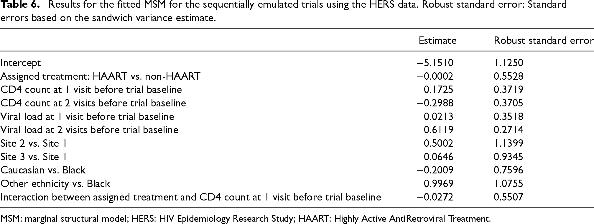
The pooled logistic regression for the MSM included an intercept term, main effect of treatment, main effects of CD4 count and HIV viral load at previous two visits before the trial baseline, main effects of ethnicity and study sites, and the interaction between treatment and CD4 count at the visit before trial baseline. A summary of the fitted MSM is provided in Table 6.
Results for the fitted MSM for the sequentially emulated trials using the HERS data. Robust standard error: Standard errors based on the sandwich variance estimate.
Results for the fitted MSM for the sequentially emulated trials using the HERS data. Robust standard error: Standard errors based on the sandwich variance estimate.
MSM: marginal structural model; HERS: HIV Epidemiology Research Study; HAART: Highly Active AntiRetroviral Treatment.
We used 500 bootstrap samples for Nonparametric and LEF bootstrap CIs, and drew a sample of size
Figure 5 presents the estimated MRD, which is the difference in risk of all-cause mortality when all patients eligible to trial 0 adhere to the treatment strategies assigned (HAART vs. no HAART). Figure 5 also includes pointwise 95% CIs of the MRD at each trial visit obtained by the four methods described in Section 4. We note that the results are not statistically significant given that all four CIs include zero.
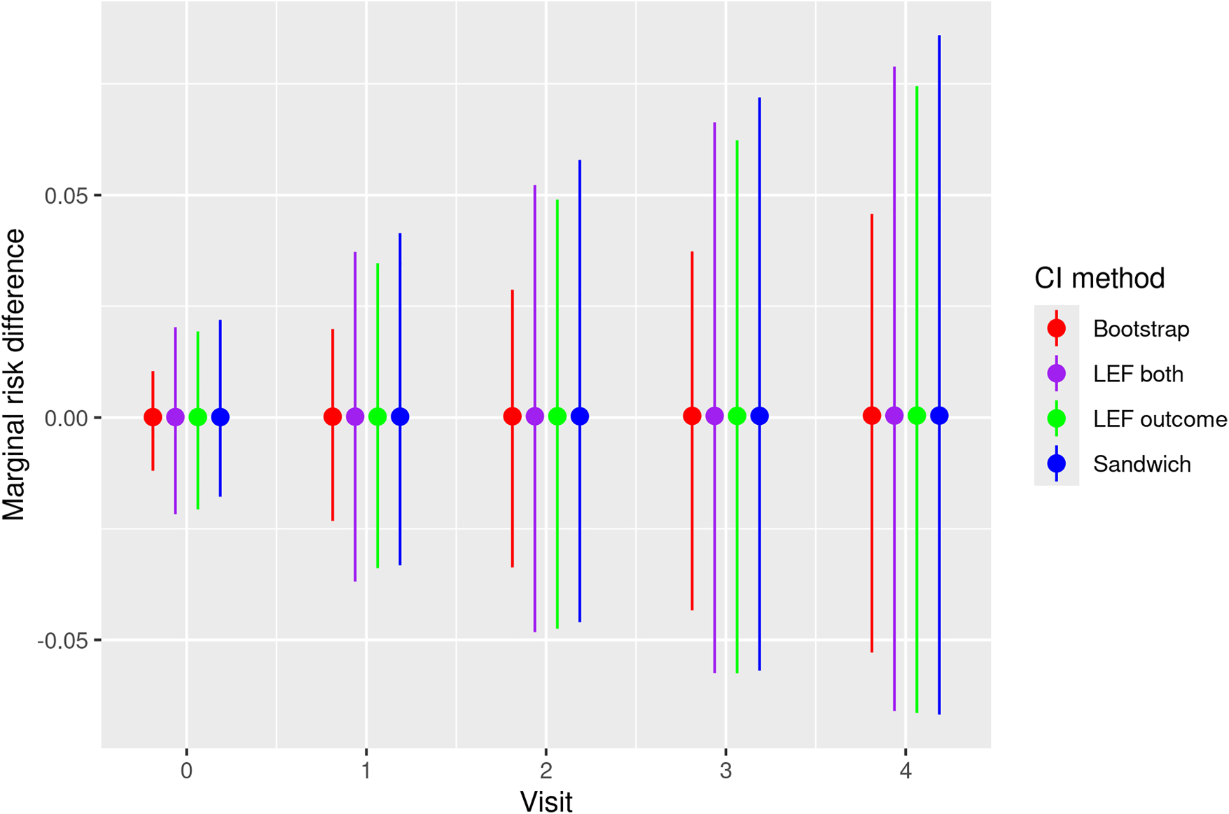
Estimates and pointwise 95% CIs of the MRD of all-cause mortality under HAART treatment strategy and the non-HAART strategy for patients enrolled in the first emulated trial (trial 0) of the HERS data. Bootstrap: CIs constructed by nonparametric bootstrap. LEF both: CIs constructed by applying Approach 2 of LEF bootstrap. LEF outcome: CIs constructed by applying Approach 1 of LEF bootstrap. Sandwich: CIs based on the sandwich variance estimator. CI: confidence interval; MRD: marginal risk difference; HAART: Highly Active AntiRetroviral Treatment; LEF: linearised estimating function; HERS: HIV Epidemiology Research Study.
In this article, we focussed on the application of STE to estimate and make inferences about the per-protocol effect of treatments on a survival outcome in terms of counterfactual MRDs over time. We conducted a simulation study to compare the relative performance of four CI construction methods for the MRD, based on the sandwich variance estimator, nonparametric bootstrap, LEF bootstrap (which previously had not been extended to STE) and jackknife resampling. In scenarios with small/medium sample sizes, low/medium event rates and low/medium treatment prevalence, we observed relatively better coverage for LEF bootstrap CIs than for nonparametric bootstrap and Sandwich CIs. These results align with previous findings on the limitations of the sandwich variance estimator when the sample size is small.47,48 Since STE is particularly useful in scenarios with small sample sizes, low event rates and low treatment prevalence, the LEF bootstrap offers a valuable alternative to the sandwich variance estimator and the nonparametric bootstrap for constructing CIs of the MRD. With large sample sizes and medium/high event rates, Sandwich CIs exhibited relatively better performance in our simulations and were also computationally more efficient, therefore one could choose to use them in such scenarios. Our simulation results also highlighted how data sparsity issues which are inherent when implementing STE can greatly affect CI performance, meaning that one should carefully consider features of their data when choosing a CI method.
Although dependent censoring was not included in the data generating mechanism of our simulation study, we expect that the relative performance of CIs constructed using LEF bootstrap and the sandwich variance estimator observed in our simulation study would also hold if there were dependent censoring and IPCWs were used to handle it. Inference would still face the same issues, but with the additional uncertainty caused by the estimation of IPCWs and possible exacerbation of the finite-sample bias as a result of loss of information.
We primarily focussed on pooled logistic regressions for fitting MSMs and did not explore alternative survival time models, such as additive hazards models. 20 Additive hazard models can be used in moderate-to-high event rates settings, while in low event rate settings they might result in negative hazard estimates. Inference procedures for STE based on additive hazard models warrant further research.
We have used parametric models for estimation of the SIPTCWs. Recent developments in nonparametric data-adaptive methods have led to their widespread use in biomedical research. This is partly because these models have become more accessible due to increased automation in their implementation across programming languages. Because the consistency of the weighted estimators of the MSM parameters relies on correct specification of treatment and censoring models, data-adaptive methods are attractive. However, the subsequent inference can be challenging.49–54
Throughout this article, it was assumed that there were no unmeasured confounders. However, in practice, this assumption is unlikely to hold, as it is challenging to identify and measure all potential confounders in observational databases. Instrumental variable approaches and sensitivity analysis have been proposed to deal with such unmeasured confounding for point treatments. Recently, Tan (2023) proposed a sensitivity analysis approach in general longitudinal settings. 55 In the specific setting of STE, sensitivity analysis methods for unmeasured confounding warrant further research.
Supplemental Material
sj-pdf-1-smm-10.1177_09622802251356594 - Supplemental material for Inference procedures in sequential trial emulation with survival outcomes: Comparing confidence intervals based on the sandwich variance estimator, bootstrap and jackknife
Supplemental material, sj-pdf-1-smm-10.1177_09622802251356594 for Inference procedures in sequential trial emulation with survival outcomes: Comparing confidence intervals based on the sandwich variance estimator, bootstrap and jackknife by Juliette M Limozin, Shaun R Seaman and Li Su in Medical Research
Footnotes
Acknowledgements
The authors would like to thank Dr Brian Tom and Dr Pantelis Samartsidis for helpful comments and suggestions.
Funding
The authors disclosed receipt of the following financial support for the research, authorship, and/or publication of this article: Data from the HERS were collected under grant U64-CCU10675 from the U.S. Centers for Disease Control and Prevention. This work is supported by the U.K. Medical Research Council [grants MC_UU_00002/15, MC_UU_00040/03 and MC_UU_00040/05] and the MRC Biostatistics Unit Core Studentship.
Declaration of conflicting interest
The authors declared no potential conflicts of interest with respect to the research, authorship, and/or publication of this article.
Data availability
Supplemental material
Supplemental material for this article is available online.
References
Supplementary Material
Please find the following supplemental material available below.
For Open Access articles published under a Creative Commons License, all supplemental material carries the same license as the article it is associated with.
For non-Open Access articles published, all supplemental material carries a non-exclusive license, and permission requests for re-use of supplemental material or any part of supplemental material shall be sent directly to the copyright owner as specified in the copyright notice associated with the article.