Biomarker-driven optimal designs for patient enrollment restriction

Abstract

The rapidly developing field of personalized medicine is giving the opportunity to treat patients with a specific regimen according to their individual demographic, biological, or genomic characteristics, known also as biomarkers. While binary biomarkers simplify subgroup selection, challenges arise in the presence of continuous ones, which are often categorized based on data-driven quantiles. In the context of binary response trials for treatment comparisons, this paper proposes a method for determining the optimal cutoff of a continuous predictive biomarker to discriminate between sensitive and insensitive patients, based on their relative risk. We derived the optimal design to estimate such a cutoff, which requires a set of equality constraints that involve the unknown model parameters and the patients’ biomarker values and are not directly attainable. To implement the optimal design, a novel covariate-adjusted response-adaptive randomization is introduced, aimed at sequentially minimizing the Euclidean distance between the current allocation and the optimum. An extensive simulation study shows the performance of the proposed approach in terms of estimation efficiency and variance of the estimated cutoff. Finally, we show the potential severe ethical impact of adopting the data-dependent median to identify the subpopulations.

1. Introduction and model

Nowadays almost all branches of medicine are moving toward personalized medicine based on the belief that all patients cannot be successfully treated with the same therapy. In the presence of some evidence that the effect of a treatment may differ in certain subpopulations, personalized (also known as precision medicine) may be extremely useful. More precisely, personalized medicine is the tailoring of medical treatments to the individual characteristics, or biomarkers, of each patient. The process of selection of the subpopulations based on one or more biomarkers is called enrichment: subjects are screened for their biomarker profile, and then only those with or without certain characteristics are included in the trial and could be suitably randomized to the competing treatments.

While enrichment trials are specifically applied in the design phase, in terms of both enrollment restrictions and treatment allocation process, traditional subgroup identification methods are ex-post procedures for analyzing data already accrued in randomized clinical trials. The vast majority of them are classification algorithms of heuristic nature, without model specifications; they are based on classification trees combined with machine learning techniques, aimed at identifying a set of predictive biomarkers (among many available covariates, some of which are of prognostic nature) as well as suitable subsets of their support (see, e.g. Foster et al. ¹ ). Other proposals have been introduced for continuous endpoints under the classical linear model, often in the causal inference framework or inspired by latent variables approaches (see for a recent review by Loh et al. ² ).

In several cases, the effects of biomarkers on treatments are not explicit. Therefore, adaptive enrichment design methodologies, using the accrued information on previous subjects’ responses to find the benefitting population, can be applied. In the presence of a binary (or categorical) biomarker, the patients’ subgroups are well-defined. Nevertheless, when the biomarker of interest is defined on a continuous scale (e.g. age, cholesterol, and blood pressure), a widely used approach consists of discretizing the biomarker via a cutoff given by a data-driven quantile, usually the median, in order to define the subgroups. However, as stated by many authors, “discretization of a continuous biomarker using sample percentiles results in significant information loss and should be avoided” (see Polley and Dignam ³ and Zhang and Molinaro ⁴ ). Moreover, often a single candidate predictive biomarker is identified via preliminary information, but a suitable cutpoint has not been established. ⁵ Under this framework, patient enrollment restriction based on the biomarker would be inappropriate. Indeed, an erroneous identification of the threshold for guiding future treatment decisions for individual patients could lead to potentially severe consequences.

Regrettably, there is still a lack of studies that estimate the threshold directly on a continuous scale to correctly discriminate among the so-called sensitive (biomarker-positive) and insensitive (biomarker-negative) patients. ⁶ Recently, for a single-arm trial, Spencer et al. ⁷ presented a biomarker-adaptive threshold design to determine if a subpopulation with a clinically relevant response rate exists. Some proposals have been developed in the context of survival trials (see Trippa et al., ⁸ Renfro et al., ⁹ and Diao et al. ¹⁰ ). On the other hand, Lin et al. ¹¹ and Frieri et al. ¹² adopted a bivariate-normal model to estimate the biomarker threshold, using the correlation biomarker-response as an explicit gauge of the predictive nature of the biomarker. Baldi Antognini et al. ¹³ used the linear treatment-by-covariate interaction approach to find the cutoff and provide the optimal allocations for both parameter estimation and cutoff identification.

Inspired by numerous real clinical trials documented in the literature, consider as a motivating example the NSABP B-35 trial described by Margolese et al. ¹⁴ By enrolling 3104 patients, this study compares anastrozole versus tamoxifen in postmenopausal women with hormone receptor-positive ductal carcinoma in situ undergoing lumpectomy plus radiotherapy, showing that anastrozole provides a significant improvement in breast cancer-free interval in women younger than 60 years.

Since a binary model for the biomarker–treatment relationship is frequently required for therapeutic success/failure cases (see, e.g. Vinnat and Chevret ¹⁵ ), in this paper, we approach the challenging issue of identifying the optimal cutpoint of a continuous predictive biomarker based on the relative risk for binary trials for treatment comparisons. Our aim is to provide optimal allocations for inference on the threshold and then describe a suitable covariate-adjusted response-adaptive (CARA) procedure to implement this optimum. After introducing the statistical model in Section 2, Section 3 deals with classical $D$ and $A$ optimality criteria, also providing the variance of the estimated threshold. We derive the optimal design that simultaneously optimizes all the above-mentioned criteria, which consists of a set of conditions, involving the unknown patients’ biomarker values and the unknown model parameters. Thus, Section 4 is dedicated to the implementation of the optimal design through a suitably defined CARA rule. Finally, in Section 5, we perform a simulation study adopting normal and log-normal distribution for the biomarker, in order to compare the performance of the new CARA procedure with that of conventional trial designs. To stress the practical impact of our procedure, we redesign a clinical trial for severe sepsis disease, taking also into account the Virtual Twins method ¹ for subgroup identification. Additionally, the ethical impact resulting from the use of a median-based biomarker cutoff has been explored, comparing it with the benefit gained from using the relative risk-based cutoff.

2. Binary responses

We consider an oncological trial where patients are sequentially assigned to one of two competing anticancer agents $T$ or $C$ . Let us denote by $X$ the chosen quantitative predictive biomarker, which is not under the experimenters’ control. When the $i$ th subject is ready to be randomized, the biomarker value $X_i=x_i$ is recorded and she/he receives one of the agents based on a given randomization rule and a treatment indicator variable records the assignment: if the patient is assigned to $T$ , ${\delta }_i=1$ while ${\delta }_i=0$ otherwise. Thus, $n^{-1}\sum _{i=1}^n{\delta }_i=\pi$ is the subjects’ proportion allocated to $T$ and $n^{-1}\sum _{i=1}^n(1-{\delta }_i)=1-\pi$ to $C$ . We assume $X_1,X_2,\dots$ independent and identically distributed random variables having common density function with finite expected value and variance. A binary tumor status $Y_i$ is examined after the treatment assignment to directly measure any anticancer activity (e.g. the ctDNA clearance in Spreafico et al. ¹⁶ ) and we take $Y_i=1$ in the case of successful response of the $i$ th patient (clearly, this setting applies to any dichotomous outcomes of interest, such as mortality of patients with hypoxemic acute respiratory failure after different oxygenation therapies in the HIGH clinical trial, see Azoulay et al. ¹⁷ ).

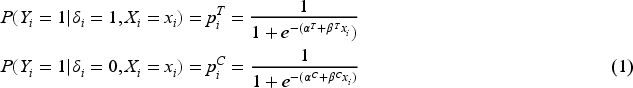
Conditionally on the treatments and the biomarker, subjects’ responses are assumed to be independent following a logistic regression model:

$$\begin{array}{rl}P(Y_i=1|{\delta }_i=1,X_i=x_i)& =p_i^T=\frac{1}{1+e^{-({\alpha }^T+{\beta }^T{x}_i})}\\ P(Y_i=1|{\delta }_i=0,X_i=x_i)& =p_i^C=\frac{1}{1+e^{-({\alpha }^C+{\beta }^C{x}_i)}}\end{array}$$

(1)

where, since $X$ is a predictive biomarker, ${\beta }^T\ne {\beta }^C$ .

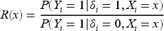
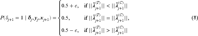
The primary goal of the paper is to assess whether an anticancer agent is better than the other for a subgroup of subjects based on their biomarker. By taking into account the relative risk,

$$R(x)=\frac{P(Y_i=1|{\delta }_i=1,X_i=x)}{P(Y_i=1|{\delta }_i=0,X_i=x)}$$

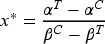
it is easy to show that, for every subject with biomarker value $x$ greater than the unique cutoff

$$x^{*}=\frac{{\alpha }^T-{\alpha }^C}{{\beta }^C-{\beta }^T}$$

agent $T$ is better than $C$ (namely $R(x)>1$ ) provided that ${\beta }^T>{\beta }^C$ (or for $x<x^{*}$ if ${\beta }^T<{\beta }^C$ ). This subpopulation of patients (often referred to as target or benefitting subpopulation) is generally the focus of the investigator assuming that $T$ is regarded as the new/experimental treatment. Moreover, after the identification of the cutoff, a secondary objective is to evaluate the impact of the discretization of the continuous biomarker using a sample percentile instead of $x^{*}$ , in terms of ethical loss (namely the percentage of subjects assigned to the inferior treatment).

As regards the notation, throughout the paper let ${\mathit{x}}_n^t=(x_1,\dots ,x_n)$ , ${\mathit{\delta }}_n^t=({\delta }_1,\dots ,{\delta }_n)$ , and ${\mathit{y}}_n^t=(y_1,\dots ,y_n)$ be the vector of biomarker values, assignments, and outcomes observed after $n$ steps and ${\mathbf{0}}_k$ is the $k$ -dimensional vector of zeros.

3. Trial designs

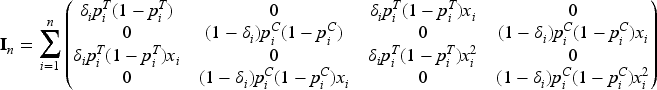
Optimal design theory is recognized as an important tool to achieve allocations that yield the best performance out of a range of potential designs. The literature is rich with optimal design methodologies that can be adopted by clinical researchers to improve the efficiency of the drug development process. The key idea is to select a criterion that measures the loss as a function of the inverse of the Fisher information matrix since it is an asymptotic approximation of the variance–covariance matrix of the maximum likelihood estimators (MLEs). Denoting by $\theta \theta =({\alpha }^T,{\alpha }^C,{\beta }^T,{\beta }^C{)}^t$ the vector of the unknown parameters, let $\hat{\theta }{\hat{\theta }}_n=({\hat{\alpha }}_n^T,{\hat{\alpha }}_n^C,{\hat{\beta }}_n^T,{\hat{\beta }}_n^C{)}^t$ be the MLE of $\theta \theta$ after $n$ steps, then the Fisher information is (see Appendix 1)

$${\mathbf{I}}_n=\sum _{i=1}^n\left(\begin{array}{cccc}{\delta }_i{p}_i^T(1-p_i^T)& 0& {\delta }_i{p}_i^T(1-p_i^T)x_i& 0\\ 0& (1-{\delta }_i)p_i^C(1-p_i^C)& 0& (1-{\delta }_i)p_i^C(1-p_i^C)x_i\\ {\delta }_i{p}_i^T(1-p_i^T)x_i& 0& {\delta }_i{p}_i^T(1-p_i^T)x_i^2& 0\\ 0& (1-{\delta }_i)p_i^C(1-p_i^C)x_i& 0& (1-{\delta }_i)p_i^C(1-p_i^C)x_i^2\end{array}\right)$$

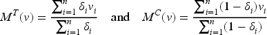
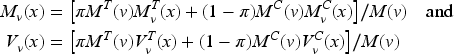
To simplify the notation, let us define the variance of the response of patient $i$ with $v_i={\delta }_i{p}_i^T(1-p_i^T)+(1-{\delta }_i)p_i^C(1-p_i^C)$ ; clearly, if ${\delta }_i=1$ then $v_i=p_i^T(1-p_i^T)$ , whereas $v_i=p_i^C(1-p_i^C)$ if ${\delta }_i=0$ . Thus, ${\delta }_i{v}_i={\delta }_i{p}_i^T(1-p_i^T)$ and $(1-{\delta }_i)v_i=(1-{\delta }_i)p_i^C(1-p_i^C)$ , so that

$$M^T(v)=\frac{\sum _{i=1}^n{\delta }_i{v}_i}{\sum _{i=1}^n{\delta }_i}\text{and}{M}^C(v)=\frac{\sum _{i=1}^n(1-{\delta }_i)v_i}{\sum _{i=1}^n(1-{\delta }_i)}$$

simply denote the means of the observed variances in the two groups. Moreover, since

$${\nu }^T=(\frac{{\delta }_i{v}_i}{\sum _{i=1}^n{\delta }_i{v}_i}:i=1,\dots ,n)\text{and}{\nu }^C=(\frac{(1-{\delta }_i)v_i}{\sum _{i=1}^n(1-{\delta }_i)v_i}:i=1,\dots ,n)$$

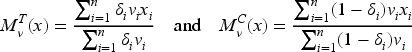
represent two discrete probability distributions, we denote by

$$M_{\nu }^T(x)=\frac{\sum _{i=1}^n{\delta }_i{v}_i{x}_i}{\sum _{i=1}^n{\delta }_i{v}_i}\text{and}{M}_{\nu }^C(x)=\frac{\sum _{i=1}^n(1-{\delta }_i)v_i{x}_i}{\sum _{i=1}^n(1-{\delta }_i)v_i}$$

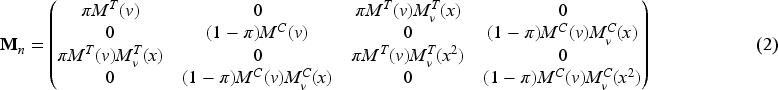
the mean of the biomarker with respect to ${\nu }^T$ and ${\nu }^C$ , respectively, with $V_{\nu }^j(x)=M_{\nu }^j(x^2)-[M_{\nu }^j(x){]}^2$ ( $j=T,C$ ) the corresponding variances. Thus, the average information matrix ${\mathbf{M}}_n={\mathbf{I}}_n/n$ is

$${\mathbf{M}}_n=\left(\begin{array}{cccc}\pi M^T(v)& 0& \pi M^T(v)M_{\nu }^T(x)& 0\\ 0& (1-\pi )M^C(v)& 0& (1-\pi )M^C(v)M_{\nu }^C(x)\\ \pi M^T(v)M_{\nu }^T(x)& 0& \pi M^T(v)M_{\nu }^T(x^2)& 0\\ 0& (1-\pi )M^C(v)M_{\nu }^C(x)& 0& (1-\pi )M^C(v)M_{\nu }^C(x^2)\end{array}\right)$$

(2)

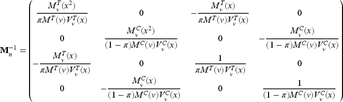
and its inverse is given by (see Appendix 2)

$${\mathbf{M}}_n^{-1}=\left(\begin{array}{cccc}{\displaystyle \frac{M_{\nu }^T(x^2)}{\pi M^T(v)V_{\nu }^T(x)}}& 0& -{\displaystyle \frac{M_{\nu }^T(x)}{\pi M^T(v)V_{\nu }^T(x)}}& 0\\ 0& {\displaystyle \frac{M_{\nu }^C(x^2)}{(1-\pi )M^C(v)V_{\nu }^C(x)}}& 0& -{\displaystyle \frac{M_{\nu }^C(x)}{(1-\pi )M^C(v)V_{\nu }^C(x)}}\\ -{\displaystyle \frac{M_{\nu }^T(x)}{\pi M^T(v)V_{\nu }^T(x)}}& 0& {\displaystyle \frac{1}{\pi M^T(v)V_{\nu }^T(x)}}& 0\\ 0& -{\displaystyle \frac{M_{\nu }^C(x)}{(1-\pi )M^C(v)V_{\nu }^C(x)}}& 0& {\displaystyle \frac{1}{(1-\pi )M^C(v)V_{\nu }^C(x)}}\end{array}\right)$$

3.1. Optimality criteria

When the interest is in the estimation of the whole parameter vector $\theta \theta$ , $D$ and $A$ optimality criteria are typically used. The former criterion minimizes the volume of the confidence ellipsoid for $\theta \theta$ , so that the $D$ optimal design minimizes the determinant of ${\mathbf{M}}_n^{-1}$ . Whereas, the $A$ optimality minimizes the mean variance of the estimators, so the trace of ${\mathbf{M}}_n^{-1}$ should be minimized. Concerning the estimation of $x^{*}$ , the MLE of the threshold after $n$ steps is ${\hat{x}}_n^{*}=({\hat{\alpha }}_n^T-{\hat{\alpha }}_n^C)/({\hat{\beta }}_n^C-{\hat{\beta }}_n^T)$ and the next theorem provides an approximated closed-form for its variance, as well as the expression of $D$ and $A$ optimality criteria.

Theorem 3.1

After $n$ assignments,

$$det\text{var}({\hat{\mathit{\theta }}}_n)=\frac{1}{{\pi }^2(1-\pi {)}^2{[M^T(v)]}^2{[M^C(v)]}^2{V}_{\nu }^T(x)V_{\nu }^C(x)}$$

(3)

and

$$\text{tr}\text{var}({\hat{\mathit{\theta }}}_n)=\frac{1+M_{\nu }^T(x^2)}{\pi M^T(v)V_{\nu }^T(x)}+\frac{1+M_{\nu }^C(x^2)}{(1-\pi )M^C(v)V_{\nu }^C(x)}$$

(4)

As regards the threshold estimation, since ${\beta }^T\ne {\beta }^C$ , through a first-order approximation,

$$\text{var}({\hat{x}}_n^{*})\approx \frac{1}{({\beta }^T-{\beta }^C{)}^2}\{\frac{\pi M^T(v)+(1-\pi )M^C(v)}{\pi (1-\pi )M^T(v)M^C(v)}+\frac{{[M_{\nu }^T(x)-x^{*}]}^2}{\pi M^T(v)V_{\nu }^T(x)}+\frac{{[M_{\nu }^C(x)-x^{*}]}^2}{(1-\pi )M^C(v)V_{\nu }^C(x)}\}$$

(5)

Proof.

See Appendix 3.

3.2. Optimal designs

Assuming model (1), the following theorem provides the optimal design for the estimation of the cutoff, which is also $D$ and $A$ optimal.

Theorem 3.2

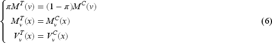
An allocation ${\mathit{\delta }}_n^{*}$ satisfying

$$\{\begin{array}{rl}\pi M^T(v)& =(1-\pi )M^C(v)\\ M_{\nu }^T(x)& =M_{\nu }^C(x)\\ V_{\nu }^T(x)& =V_{\nu }^C(x)\end{array}$$

(6)

is $D$ and $A$ optimal and is optimal for estimating the threshold $x^{*}$ as well.

Proof.

See Appendix 4.

Conditions (6) define a vast class of optimal designs through equality constraints, involving both the observed biomarker values and the unknown model parameters. In practice, optimality requires the equality of the biomarker weighted means and variances with respect to ${\nu }^T$ and ${\nu }^C$ , as well as the equality of $\pi M^T(v)$ to $(1-\pi )M^C(v)$ .

Since in our setting incoming patients’ biomarker cannot be controlled by the experimenter, given $M(v)=n^{-1}\sum _{i=1}^n{v}_i$ and the marginal quantities $M_{\nu }(x)=\sum _{i=1}^n{v}_i{x}_i/\sum _{i=1}^n{v}_i$ and $V_{\nu }(x)=M_{\nu }(x^2)-[M_{\nu }(x){]}^2$ (i.e. mean and variance evaluated w.r.t. $\nu =(v_i/\sum _{i=1}^n{v}_i:i=1,\dots ,n)$ ), the selection of $\pi ,M^T(v),M_{\nu }^T(x)$ and $V_{\nu }^T(x)$ uniquely determines $(1-\pi ),M^C(v),M_{\nu }^C(x)$ and $V_{\nu }^C(x)$ :

$$\begin{array}{rl}M(v)& =\pi M^T(v)+(1-\pi )M^C(v),\end{array}$$

(7)

$$\begin{array}{rl}{M}_{\nu }(x)& =[\pi M^T(v)M_{\nu }^T(x)+(1-\pi )M^C(v)M_{\nu }^C(x)]/M(v)\text{and}\\ V_{\nu }(x)& =[\pi M^T(v)V_{\nu }^T(x)+(1-\pi )M^C(v)V_{\nu }^C(x)]/M(v)\end{array}$$

Thus, conditions (6) can be restated as $2\pi M^T(v)=M(v)$ , $M_{\nu }^T(x)=M_{\nu }(x)$ , $V_{\nu }^T(x)=V_{\nu }(x)$ . If, in addition, a balanced allocation $\pi =1/2$ is assumed, the optimum requires $M(v)=M^T(v)=M^C(v)$ and clearly $M_{\nu }^T(x)=M_{\nu }^C(x)=M_{\nu }(x)$ and $V_{\nu }^T(x)=V_{\nu }^C(x)=V_{\nu }(x)$ .

The dependence of the optimal designs (derived in Theorem 3.2) on the unknown model parameters is highlighted in the next remark.

Remark 3.1

Unlike the results obtained in Baldi Antognini et al., ¹³ conditions (6) cannot be achieved in practice, since they depend on all the observed allocations and biomarker values, as well as on the unknown model parameter $\mathit{\theta }$ . Thus, even in the unrealistic scenario in which the experimenter could be able to choose the biomarker values of the subjects, the closeness to the optimum cannot be checked since it depends on $\mathit{\theta }$ . Indeed, consider the following toy example with $n=4$ , where we assume ${\mathit{x}}_4=(0,0,0.8,0.8{)}^t$ and ${\mathit{\delta }}_4=(0,1,0,1{)}^t$ . In such a case $\pi =1/2$ , $\sum _{i=1}^4{\delta }_i{x}_i=\sum _{i=1}^4(1-{\delta }_i)x_i=0.8$ and $\sum _{i=1}^4{\delta }_i{x}_i^2=\sum _{i=1}^4(1-{\delta }_i)x_i^2=0.64$ , so the equality between the first and second empirical moments of the biomarker is achieved. When ${\mathit{\theta }}^t=(-0.5,0.2,1.2,0.2)$ (i.e. $x^{*}=0.7$ ), conditions (6) are satisfied with $M^T(v)=M^C(v)=0.24$ , $M_{\nu }^T(x)=M_{\nu }^C(x)=0.40$ , and $V_{\nu }^T(x)=V_{\nu }^C(x)=0.16$ . However, if ${\mathit{\theta }}^t=(1.8,2.5,1.8,0.8)$ (inducing the same threshold $x^{*}=0.7$ ), then the considered allocation ${\mathit{\delta }}_4$ is not optimal since $M^T(v)=0.08\ne M^C(v)=0.05$ , $M_{\nu }^T(x)=0.18\ne M_{\nu }^C(x)=0.29$ , and $V_{\nu }^T(x)=0.11\ne V_{\nu }^C(x)=0.15$ . Moreover, under this choice of $\mathit{\theta }$ does not exist an allocation satisfying conditions (6).

4. CARA procedure to implement the optimum

As pointed out previously, the optimal designs derived in Theorem 3.2 depend on the patients’ biomarker values and the unknown model parameters. In these settings, CARA randomization could provide a possible solution to asymptotically approach the optimum. However, standard CARA procedures proposed in the literature are based on a target, namely on the complete specification of the functional form of the optimal design (see, e.g. Baldi Antognini and Giovagnoli ¹⁸ ) and they are not applicable in this setting, where optimality is characterized only by equality constraints. Thus, we now propose a new CARA randomization procedure to achieve the optimum in a sequential manner. From (6), the optimal design requires that

$${\mathit{\lambda }}^t=(\pi M^T(v)-(1-\pi )M^C(v),M_{\nu }^T(x)-M_{\nu }^C(x),M_{\nu }^T(x^2)-M_{\nu }^C(x^2))={\mathbf{0}}_3$$

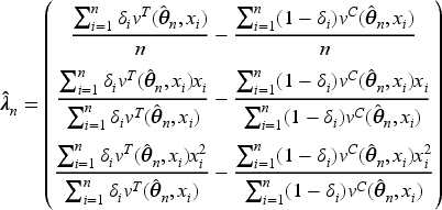
so we suggest the biomarker-adjusted response-adaptive (BiomARA) to minimize the Euclidean norm $\Vert \mathit{\lambda }\Vert =\sqrt{{\mathit{\lambda }}^t\mathit{\lambda }}$ sequentially. It goes without saying that $\mathit{\lambda }$ depends, at each step $n$ , on the set of collected allocations and patients’ biomarker values, as well as on the unknown $\mathit{\theta }$ , namely ${\mathit{\lambda }}_n=\mathit{\lambda }({\mathit{x}}_n;{\mathit{\delta }}_n;\mathit{\theta })$ , so it needs to be sequentially estimated taking also into account patients’ responses. To stress this dependence, from now on we let for every $i\ge 1$ $p_i^j=p^j(\mathit{\theta },x_i)$ and $v^j(\mathit{\theta },x_i)=p^j(\mathit{\theta },x_i)[1-p^j(\mathit{\theta },x_i)]$ , with $j=T,C$ . After $n$ assignments, we could evaluate the current MLE ${\hat{\mathit{\theta }}}_n$ of $\mathit{\theta }$ and so estimate all the previous individual success probabilities and response variances, respectively, by

$${(p^j({\hat{\mathit{\theta }}}_n,x_i))}_{i=1,\dots ,n}\text{and}{(v^j({\hat{\mathit{\theta }}}_n,x_i))}_{i=1,\dots ,n},\text{for }j=T,C$$

Thus, $\mathit{\lambda }$ can be estimated via

$${\hat{\mathit{\lambda }}}_n=\left(\begin{array}{c}{\displaystyle \frac{\sum _{i=1}^n{\delta }_i{v}^T({\hat{\mathit{\theta }}}_n,x_i)}{n}}-{\displaystyle \frac{\sum _{i=1}^n(1-{\delta }_i)v^C({\hat{\mathit{\theta }}}_n,x_i)}{n}}\\ {\displaystyle \frac{\sum _{i=1}^n{\delta }_i{v}^T({\hat{\mathit{\theta }}}_n,x_i)x_i}{\sum _{i=1}^n{\delta }_i{v}^T({\hat{\mathit{\theta }}}_n,x_i)}}-{\displaystyle \frac{\sum _{i=1}^n(1-{\delta }_i)v^C({\hat{\mathit{\theta }}}_n,x_i)x_i}{\sum _{i=1}^n(1-{\delta }_i)v^C({\hat{\mathit{\theta }}}_n,x_i)}}\\ {\displaystyle \frac{\sum _{i=1}^n{\delta }_i{v}^T({\hat{\mathit{\theta }}}_n,x_i)x_i^2}{\sum _{i=1}^n{\delta }_i{v}^T({\hat{\mathit{\theta }}}_n,x_i)}}-{\displaystyle \frac{\sum _{i=1}^n(1-{\delta }_i)v^C({\hat{\mathit{\theta }}}_n,x_i)x_i^2}{\sum _{i=1}^n(1-{\delta }_i)v^C({\hat{\mathit{\theta }}}_n,x_i)}}\end{array}\right)$$

and the BiomARA procedure can be implemented according to the following algorithm:

• Step 0:

  assign $n_0$ patients with restricted randomization to $T$ and $C$ and set $j=n_0$ ;

  Step 1:

  based on ${\mathit{x}}_j$ , ${\mathit{\delta }}_j$ and ${\mathit{y}}_j$ , estimate $\mathit{\theta }$ via ${\hat{\mathit{\theta }}}_j$ ;

  Step 2:

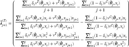
  when the $(j+1)$ th patient arrives with biomarker value $x_{j+1}$ , calculate $v^T({\hat{\mathit{\theta }}}_j,x_{j+1})$ and $v^C({\hat{\mathit{\theta }}}_j,x_{j+1})$ in order to evaluate the potential distances $||{\hat{\mathit{\lambda }}}_{j+1}^{(T)}||$ and $||{\hat{\mathit{\lambda }}}_{j+1}^{(C)}||$ from the optimum that will occur by assigning $T$ or $C$ to this subject, where

  -

  if ${\delta }_{j+1}=1$

  $${\hat{\mathit{\lambda }}}_{j+1}^{(T)}=\left(\begin{array}{c}{\displaystyle \frac{\sum _{i=1}^j{\delta }_i{v}^T({\hat{\mathit{\theta }}}_j,x_i)+v^T({\hat{\mathit{\theta }}}_j,x_{j+1})}{j+1}}-{\displaystyle \frac{\sum _{i=1}^j(1-{\delta }_i)v^C({\hat{\mathit{\theta }}}_j,x_i)}{j+1}}\\ {\displaystyle \frac{\sum _{i=1}^j{\delta }_i{v}^T({\hat{\mathit{\theta }}}_j,x_i)x_i+v^T({\hat{\mathit{\theta }}}_j,x_{j+1})x_{j+1}}{\sum _{i=1}^j{\delta }_i{v}^T({\hat{\mathit{\theta }}}_j,x_i)+v^T({\hat{\mathit{\theta }}}_j,x_{j+1})}}-{\displaystyle \frac{\sum _{i=1}^j(1-{\delta }_i)v^C({\hat{\mathit{\theta }}}_j,x_i)x_i}{\sum _{i=1}^j(1-{\delta }_i)v^C({\hat{\mathit{\theta }}}_j,x_i)}}\\ {\displaystyle \frac{\sum _{i=1}^j{\delta }_i{v}^T({\hat{\mathit{\theta }}}_j,x_i)x_i^2+v^T({\hat{\mathit{\theta }}}_j,x_{j+1})x_{j+1}^2}{\sum _{i=1}^j{\delta }_i{v}^T({\hat{\mathit{\theta }}}_j,x_i)+v^T({\hat{\mathit{\theta }}}_j,x_{j+1})}}-{\displaystyle \frac{\sum _{i=1}^j(1-{\delta }_i)v^C({\hat{\mathit{\theta }}}_j,x_i)x_i}{\sum _{i=1}^j(1-{\delta }_i)v^C({\hat{\mathit{\theta }}}_j,x_i^2)}}\end{array}\right)$$

  -

  if ${\delta }_{j+1}=0$

  $${\hat{\mathit{\lambda }}}_{j+1}^{(C)}=\left(\begin{array}{c}{\displaystyle \frac{\sum _{i=1}^j{\delta }_i{v}^T({\hat{\mathit{\theta }}}_j,x_i)}{j+1}}-{\displaystyle \frac{\sum _{i=1}^j(1-{\delta }_i)v^C({\hat{\mathit{\theta }}}_j,x_i)+v^C({\hat{\mathit{\theta }}}_j,x_{j+1})}{j+1}}\\ {\displaystyle \frac{\sum _{i=1}^j{\delta }_i{v}^T({\hat{\mathit{\theta }}}_j,x_i)x_i}{\sum _{i=1}^j{\delta }_i{v}^T({\hat{\mathit{\theta }}}_j,x_i)}}-{\displaystyle \frac{\sum _{i=1}^j(1-{\delta }_i)v^C({\hat{\mathit{\theta }}}_j,x_i)x_i+v^C({\hat{\mathit{\theta }}}_j,x_{j+1})x_{j+1}}{\sum _{i=1}^j(1-{\delta }_i)v^C({\hat{\mathit{\theta }}}_j,x_i)+v^C({\hat{\mathit{\theta }}}_j,x_{j+1})}}\\ {\displaystyle \frac{\sum _{i=1}^j{\delta }_i{v}^T({\hat{\mathit{\theta }}}_j,x_i)x_i^2}{\sum _{i=1}^j{\delta }_i{v}^T({\hat{\mathit{\theta }}}_j,x_i)}}-{\displaystyle \frac{\sum _{i=1}^j(1-{\delta }_i)v^C({\hat{\mathit{\theta }}}_j,x_i)x_i^2+v^C({\hat{\mathit{\theta }}}_j,x_{j+1})x_{j+1}^2}{\sum _{i=1}^j(1-{\delta }_i)v^C({\hat{\mathit{\theta }}}_j,x_i)+v^C({\hat{\mathit{\theta }}}_j,x_{j+1})}}\end{array}\right)$$

  Step 3:

  assign the $(j+1)$ th patient to $T$ with probability

  $$P({\delta }_{j+1}=1\mid {\mathit{\delta }}_j,{\mathit{y}}_j,{\mathit{x}}_{j+1})=\{\begin{array}{ll}0.5+ϵ,& \text{if }||{\hat{\mathit{\lambda }}}_{j+1}^{(T)}||<||{\hat{\mathit{\lambda }}}_{j+1}^{(C)}||\\ 0.5,& \text{if }||{\hat{\mathit{\lambda }}}_{j+1}^{(T)}||=||{\hat{\mathit{\lambda }}}_{j+1}^{(C)}||,\\ 0.5-ϵ,& \text{if }||{\hat{\mathit{\lambda }}}_{j+1}^{(T)}||>||{\hat{\mathit{\lambda }}}_{j+1}^{(C)}||\end{array}$$

  (8)

  where $ϵ\in (0,0.5)$ , and then observe $y_{j+1}$ .

  Set $j=j+1$ and repeat Steps 1–3 until the enrollment process is completed.

  It is important to notice that, at Step 2, the response of the $(j+1)$ th patient is yet to be observed, so $v^T({\hat{\mathit{\theta }}}_j,x_{j+1})$ and $v^C({\hat{\mathit{\theta }}}_j,x_{j+1})$ depend on the biomarker value of patient $j+1$ but are calculated via ${\hat{\mathit{\theta }}}_j$ .

  Given the allocation function in (8), the experimenter is able to control the degree of randomness of the procedure through $ϵ$ . At the extremes, the BiomARA with $ϵ=0$ coincides with the completely randomized design, while for $ϵ=0.5$ the procedure becomes deterministic.

  5. Simulation results

  To show the performances of the BiomARA, the present section is dedicated to its operating characteristics via an extensive simulation study. The suggested CARA procedure is implemented under several experimental scenarios corresponding to various hypothetical clinical settings, also in comparison with the permuted block design (PBD) having block size 4 and the complete randomization (CR), as standard benchmarks commonly used in practice. The patients’ biomarker $X$ has been simulated under two different distributions: a standard normal $N(0,1)$ and, to take into account a nonsymmetrical distribution on ${\mathbb{R}}^{+}$ , a log-normal (LN) distribution such that $\ln (X)\sim N(0,1)$ . For each scenario, we simulate 10,000 trials and we explore the behavior of BiomARA with $ϵ=0.3$ and $0.4$ , denoted by BiomARA ${}_{0.3}$ and BiomARA ${}_{0.4}$ , respectively.

  5.1. Efficiencies

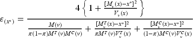
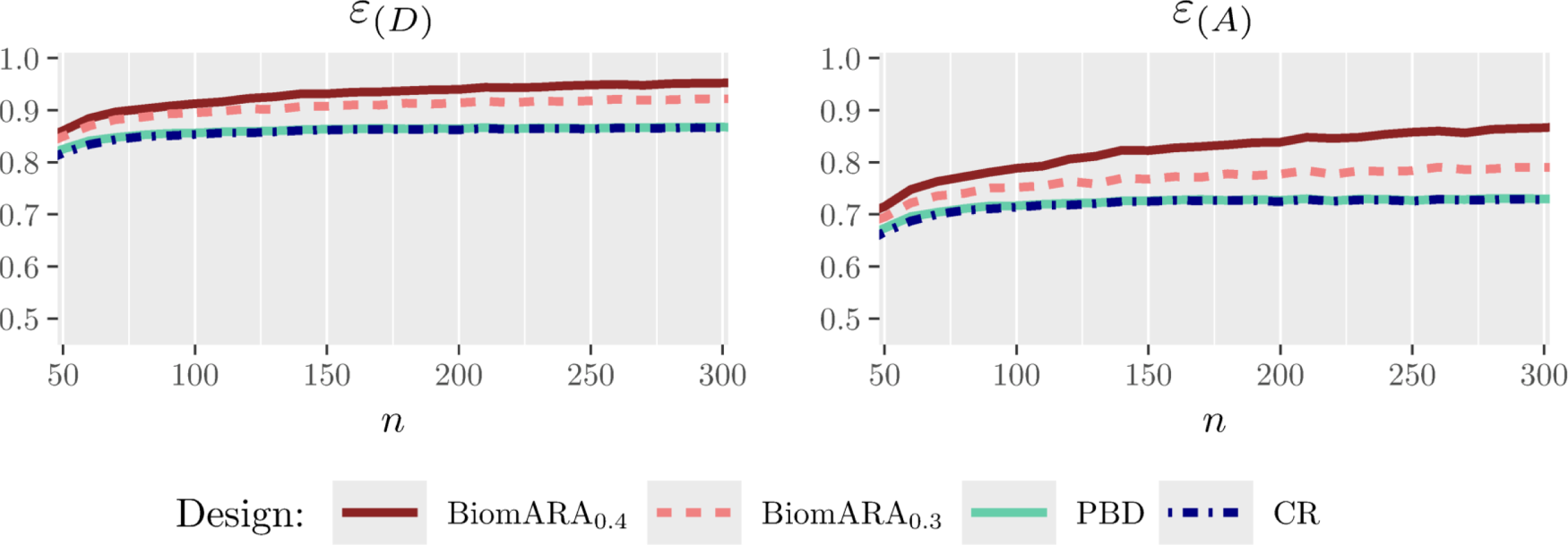
  To evaluate the relative efficiencies of a specific design, we consider $D$ and $A$ efficiency, denoted by ${\epsilon }_{(D)}$ and ${\epsilon }_{(A)}$ , whose analytical expressions are reported in Appendix B. These measures are used to compare a design with the optimum in terms of the corresponding criteria, with values equal to 1 in the case of maximum efficiency (see e.g. Atkinson et al. ¹⁹ ). Analogously, a measure of efficiency in terms of threshold estimation ${\epsilon }_{(x^{*})}$ could be defined as the ratio of the variance in (5) calculated in the optimum (6) and its value in a generic design, that is,

  $${\epsilon }_{(x^{*})}=\frac{4\{1+\frac{[M_{\nu }(x)-x^{*}{]}^2}{V_{\nu }(x)}\}}{\frac{M(v)}{\pi (1-\pi )M^T(v)M^C(v)}+\frac{[M_{\nu }^T(x)-x^{*}{]}^2}{\pi M^T(v)V_{\nu }^T(x)}+\frac{[M_{\nu }^C(x)-x^{*}{]}^2}{(1-\pi )M^C(v)V_{\nu }^C(x)}}$$
  Adopting the optimal designs in (6) implemented via the BiomARA, we simulate the behavior of the above-mentioned efficiency measures, also including CR and PBD.

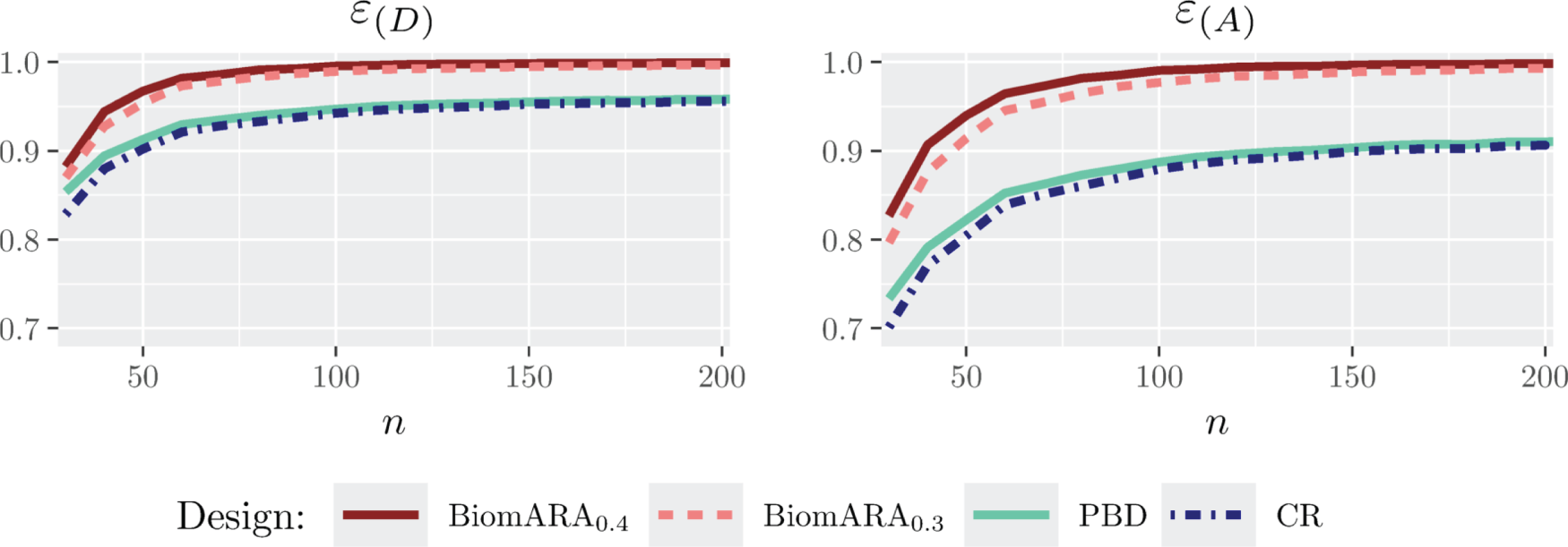
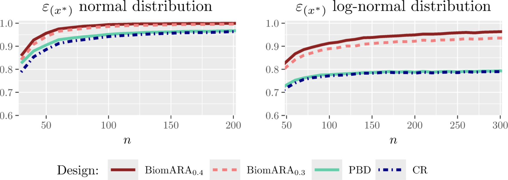
  Figure 1 and the left panel of Figure 2 show the results for the standard normal distribution with ${\mathit{\theta }}^t=(0,0.3,1.2,0.1)$ as $n$ varies between $30$ and $200$ . Whereas, Figure 3 and the right panel of Figure 2 illustrate the results under the LN distribution with ${\mathit{\theta }}^t=(-2,0,1.2,0.2)$ for $n$ between $50$ and $300$ . In both cases, BiomARA always shows a significant gain in terms of efficiency with respect to PBD and CR. Contrary to the behavior of PBD and CR, the efficiency under BiomARA increases as $n$ grows and, for the normal biomarker, reaches its maximum value even for very small sample sizes.

  Since PBD and CR have similar performance in terms of all the measures of efficiency and in accordance with the recent literature concerning the selection of the biasing probability in the presence of covariates (see e.g. Ma and Hu ²⁰ ), in the following simulations we omit both CR and BiomARA ${}_{0.3}$ .

  
  Figure 1.

  $D$ and $A$ efficiency for standard normal biomarker distribution and $\mathit{\theta }=(0,0.3,1.2,0.1{)}^t$ .

  
  Figure 2.

  Efficiency of threshold estimation ${\epsilon }_{(x^{*})}$ when the biomarker has a standard normal distribution and $\mathit{\theta }=(0,0.3,1.2,0.1{)}^t$ (left panel) and when the biomarker has a log-normal distribution and $\mathit{\theta }=(-2,0,1.2,0.2{)}^t$ (right panel).

  
  Figure 3.

  $D$ and $A$ efficiency for log-normal biomarker distribution and $\mathit{\theta }=(-2,0,1.2,0.2{)}^t$ .

  5.2. Variance of the estimated cutoff

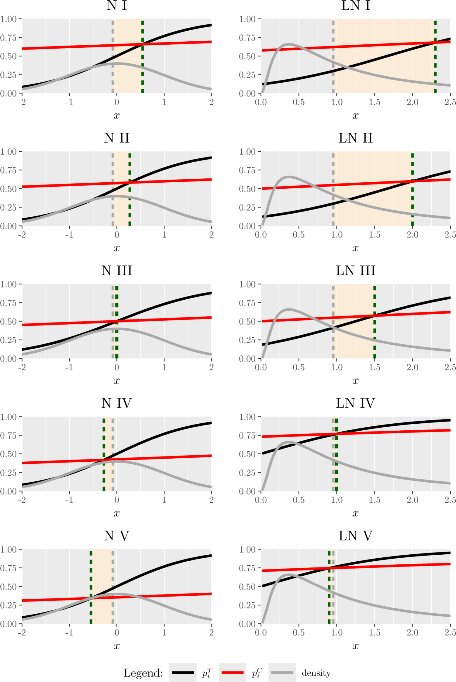
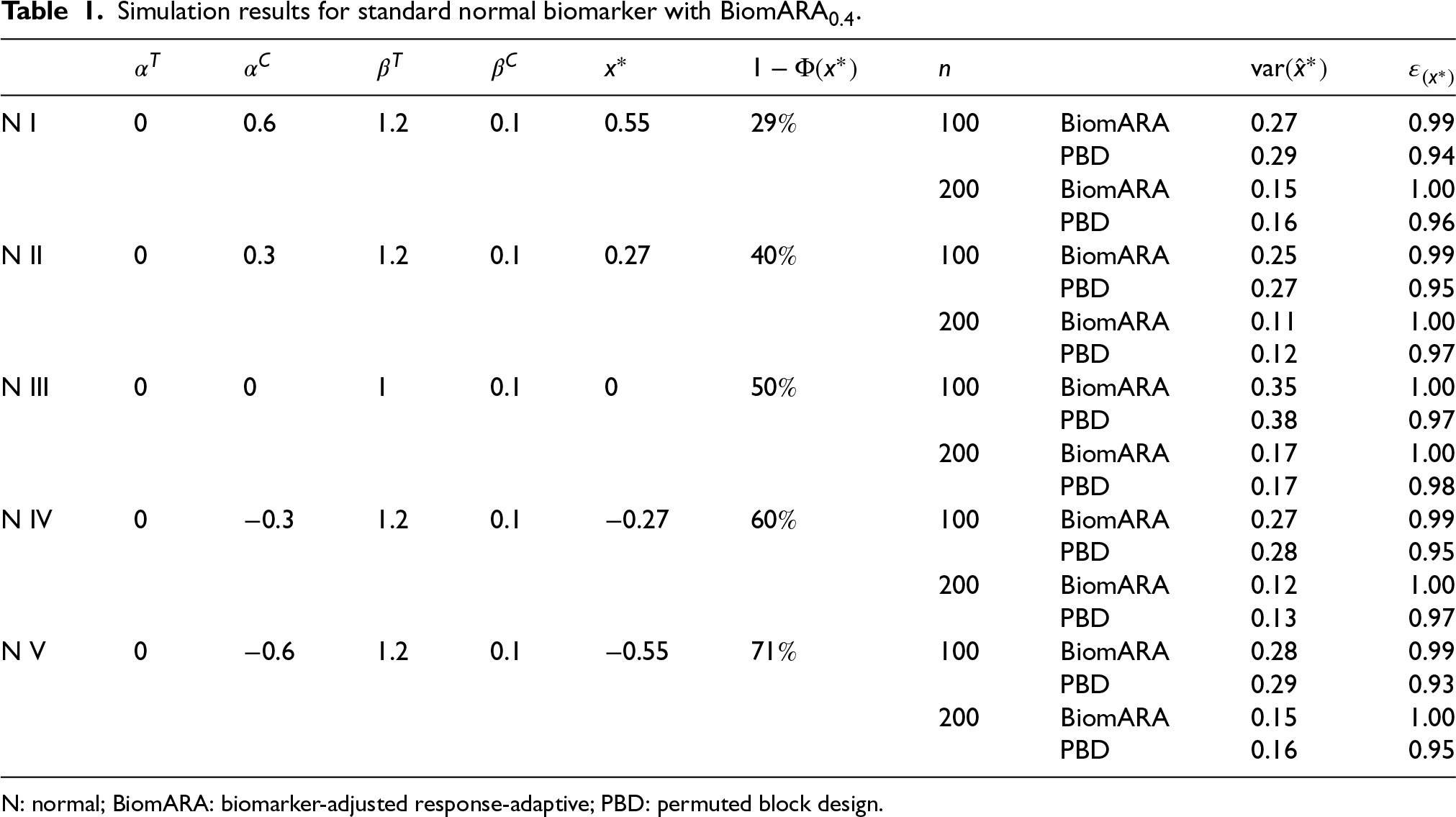
  Focusing on inference on the threshold, we now consider five experimental scenarios (N I–N V), taking a standard normal biomarker with $n=100$ and $200$ . For each scenario (represented graphically in the left panel of Figure 4), in Table 1, we report $\mathit{\theta }$ , the true threshold $x^{*}$ and $1-\mathrm{\Phi }(x^{*})$ , namely the probability for a subject to have biomarker value greater than $x^{*}$ and so to benefit from $T$ (since ${\beta }^T>{\beta }^C$ ). From N I to N V, the value of $x^{*}$ decreases and thus the reported results refer to an increasing proportion of patients benefitting from $T$ , to mimic a range of possible real clinical settings. BiomARA ${}_{0.4}$ and PBD are compared in terms of the empirical variance of the estimated threshold and the corresponding efficiency. In general, $\text{{var}}({\hat{x}}^{*})$ takes smaller values under our procedure with respect to those under PBD and BiomARA shows always higher values of ${\epsilon }_{(x^{*})}$ that reach the maximum for $n=200$ .

  
  Figure 4.

  Biomarker density function and success probabilities of $T$ (black curve) and $C$ (red curve) as $x$ varies. The displayed vertical lines correspond to the estimated median (grey dashed) and ${\hat{x}}^{*}$ (green dashed).

  
  Figure 5.

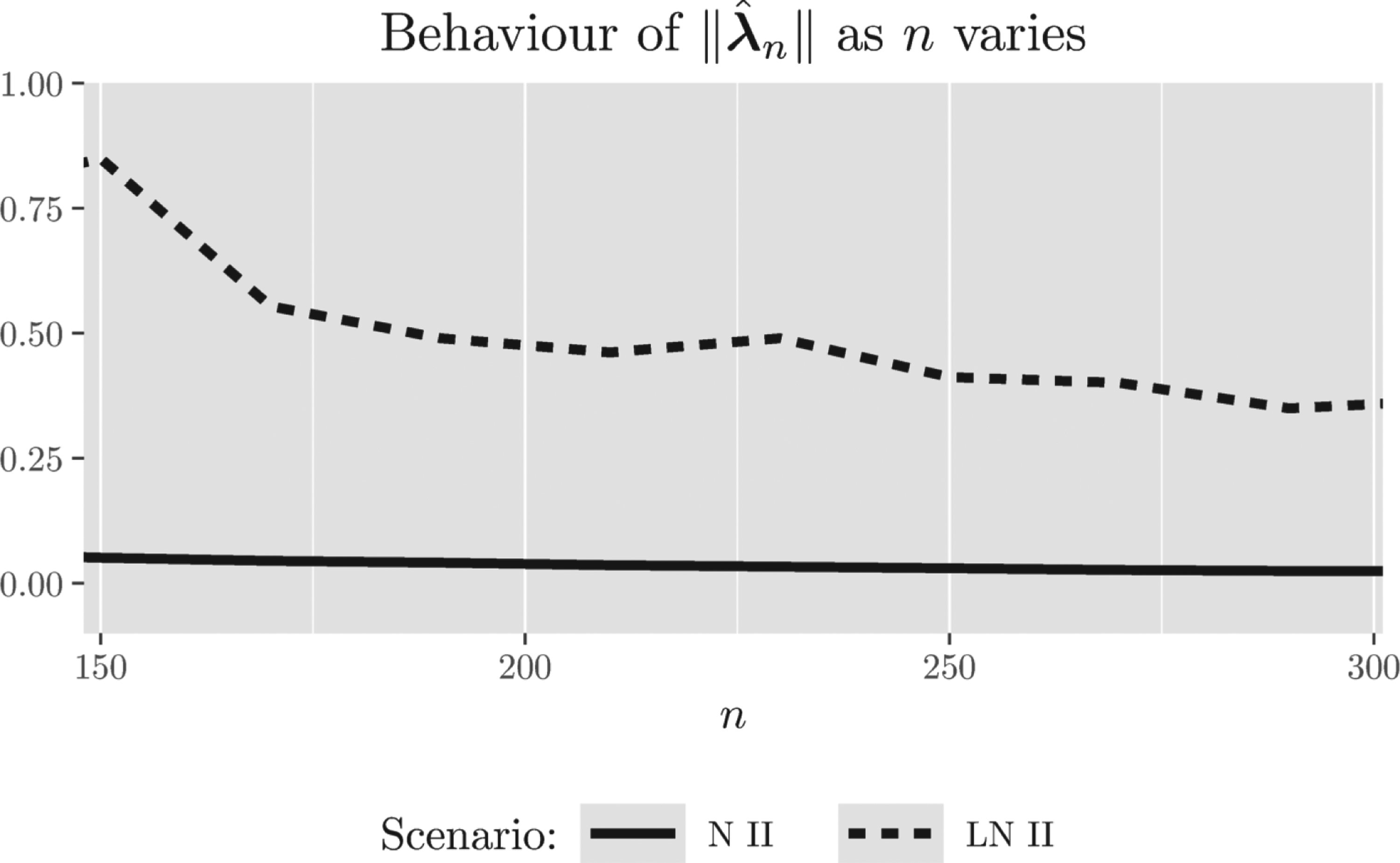
  Behavior of $\Vert {\hat{\mathit{\lambda }}}_n\Vert$ as $n$ increases for scenarios N II and LN II. N: normal; LN: log-normal.

  Table 1.

  Simulation results for standard normal biomarker with BiomARA ${}_{0.4}$ .

  

  	${\alpha }^T$	${\alpha }^C$	${\beta }^T$	${\beta }^C$	$x^{*}$	$1-\mathrm{\Phi }(x^{*})$	$n$		$\text{{var}}({\hat{x}}^{*})$	${\epsilon }_{(x^{*})}$
  N I	0	0.6	1.2	0.1	$0.55$	$29\mathrm{\%}$	100	BiomARA	0.27	0.99
  								PBD	0.29	0.94
  							200	BiomARA	0.15	1.00
  								PBD	0.16	0.96
  N II	0	0.3	1.2	0.1	$0.27$	$40\mathrm{\%}$	100	BiomARA	0.25	0.99
  								PBD	0.27	0.95
  							200	BiomARA	0.11	1.00
  								PBD	0.12	0.97
  N III	0	0	1	0.1	0	$50\mathrm{\%}$	100	BiomARA	0.35	1.00
  								PBD	0.38	0.97
  							200	BiomARA	0.17	1.00
  								PBD	0.17	0.98
  N IV	0	$-$ 0.3	1.2	0.1	$-0.27$	$60\mathrm{\%}$	100	BiomARA	0.27	0.99
  								PBD	0.28	0.95
  							200	BiomARA	0.12	1.00
  								PBD	0.13	0.97
  N V	0	$-$ 0.6	1.2	0.1	$-0.55$	$71\mathrm{\%}$	100	BiomARA	0.28	0.99
  								PBD	0.29	0.93
  							200	BiomARA	0.15	1.00
  								PBD	0.16	0.95

  N: normal; BiomARA: biomarker-adjusted response-adaptive; PBD: permuted block design.

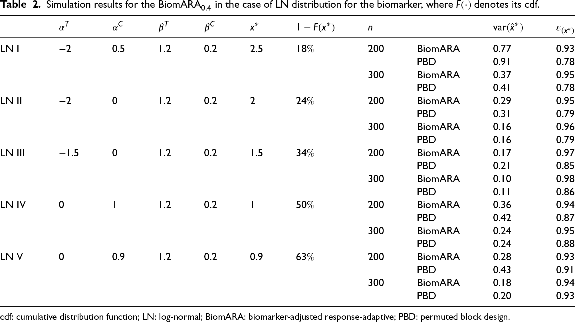
  Under the LN distribution for the biomarker, we take into account five different scenarios (LN I–LN V), represented graphically in the right panel of Figure 4: the results are reported in Table 2 for $n=200$ and $300$ . With regard to $\text{{var}}({\hat{x}}^{*})$ , similar considerations to the normal distribution case hold, while ${\epsilon }_{(x^{*})}$ seems to grow slower with $n$ , as already observed in the right panel of Figure 2.

  Table 2.

  Simulation results for the BiomARA ${}_{0.4}$ in the case of LN distribution for the biomarker, where $F(\cdot )$ denotes its cdf.

  

  	${\alpha }^T$	${\alpha }^C$	${\beta }^T$	${\beta }^C$	$x^{*}$	$1-F(x^{*})$	$n$		$\text{{var}}({\hat{x}}^{*})$	${\epsilon }_{(x^{*})}$
  LN I	$-2$	$0.5$	$1.2$	$0.2$	$2.5$	$18\mathrm{\%}$	200	BiomARA	0.77	0.93
  								PBD	0.91	0.78
  							300	BiomARA	0.37	0.95
  								PBD	0.41	0.78
  LN II	$-2$	$0$	$1.2$	$0.2$	$2$	$24\mathrm{\%}$	200	BiomARA	0.29	0.95
  								PBD	0.31	0.79
  							300	BiomARA	0.16	0.96
  								PBD	0.16	0.79
  LN III	$-1.5$	$0$	$1.2$	$0.2$	$1.5$	$34\mathrm{\%}$	200	BiomARA	0.17	0.97
  								PBD	0.21	0.85
  							300	BiomARA	0.10	0.98
  								PBD	0.11	0.86
  LN IV	$0$	$1$	$1.2$	$0.2$	$1$	$50\mathrm{\%}$	200	BiomARA	0.36	0.94
  								PBD	0.42	0.87
  							300	BiomARA	0.24	0.95
  								PBD	0.24	0.88
  LN V	$0$	$0.9$	$1.2$	$0.2$	$0.9$	$63\mathrm{\%}$	200	BiomARA	0.28	0.93
  								PBD	0.43	0.91
  							300	BiomARA	0.18	0.94
  								PBD	0.20	0.93

  cdf: cumulative distribution function; LN: log-normal; BiomARA: biomarker-adjusted response-adaptive; PBD: permuted block design.

  In general, the introduced BiomARA procedure converges to the suggested optimal designs, due to the independent and identically distributed nature of the covariate process that guarantees a stabilizing behavior for large samples (by the strong law of large numbers); however, the speed of convergence seems to be strongly related to the symmetry of the covariate distribution: Figure 5 shows the decreasing behavior of $\Vert {\hat{\mathit{\lambda }}}_n\Vert$ as $n$ grows for N II and LN II. The same graphical representation has been observed in all the other settings, omitted here for brevity, especially due to the slower convergence of the estimators in the asymmetric scenarios.

  Note that, due to the variability in the estimation of $\mathit{\theta }$ (especially for small sample sizes or when $x^{*}$ is closer to the extremes of the support of the biomarker distribution), some of the simulated trials may end with the erroneous conclusion that no threshold exists (namely the estimated threshold is outside the range of variation of the biomarker). In these cases, the estimated proportion of patients with biomarkers greater than the threshold is one (the whole population benefits from $T$ ) or zero (nobody benefits from $T$ ). The results of Tables 1 and 2 are achieved by omitting those runs. In practice, the proportion of simulated trials leading to an erroneous conclusion depends on the number of subjects enrolled: clearly, the more patients are enrolled, the closer the estimated threshold will be to the true value, leading to a more accurate identification of the patient benefitting subpopulation. Indeed, preliminary clinical studies for identifying subpopulations require larger sample sizes than traditional nonpersonalized medicine trials (Mackey and Bengtsson ²¹ ) and a metric based on this proportion has been used as a criterion to select the sample size (see Frieri et al. ¹² ). In the presented simulation study, we investigated only settings in which the percentage of reaching a wrong conclusion was lower than $5\mathrm{\%}$ . Based on this, higher sample sizes have been set for the LN distribution.

  5.3. The ethical impact of discretizing a continuous biomarker

  In the presence of a continuous predictive biomarker, common practice has been to take its median to discriminate among the two subpopulations of biomarker-positive (sensitive) and biomarker-negative (insensitive) patients. Nevertheless, a clinical study to identify a threshold could be a preliminary stage for later phases and should determine some guidance for future use of $T$ and $C$ . ⁶ In practice, if the true threshold would be a priori known, we would assign the treatment only to patients belonging to the sensitive subpopulation. We perform a simulation study to emulate such a situation in order to show the ethical impact of taking the data-driven median as a threshold instead of the one suggested in this paper, calculated via the relative risk.

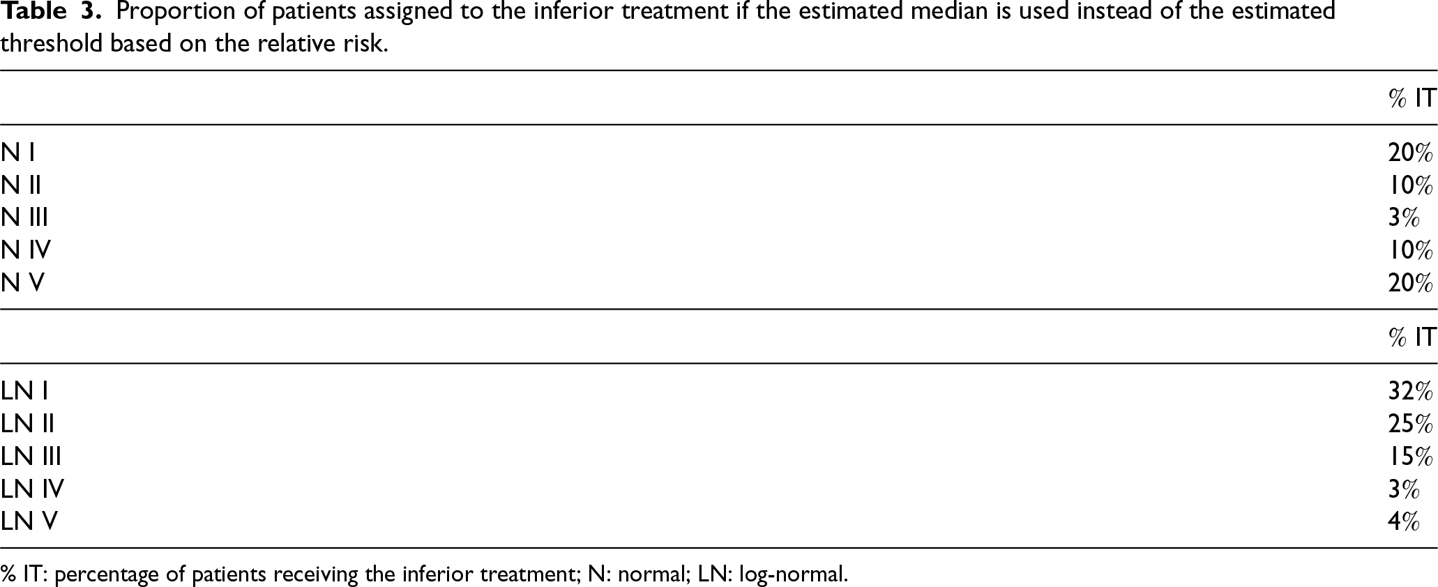
  To this end, we take into account the results obtained in Tables 1 and 2 (for $n=200$ ) as if they represent a preliminary phase through which the researcher had the opportunity to estimate both the median and the cutoff. Figure 4 describes the experimental scenarios N I–N V and LN I–LN V: the black (red) curve corresponds to the success probability of $T$ ( $C$ )—namely $p_i^T$ ( $p_i^C$ )—while the gray curve represents the standard normal density (left panel) and the LN density (right panel). Finally, the gray dashed line is the corresponding estimated median, while the green dashed line is ${\hat{x}}^{*}$ (calculated by using the estimates of model parameters found in the first phase). We simulate patients’ biomarkers and we assign them to $T$ or $C$ by using (i) the estimated median and (ii) ${\hat{x}}^{*}$ . Then, we compute the percentage of patients receiving the inferior treatment ( $\mathrm{\%}$ IT) when using the estimated median to discriminate the subpopulations, instead of ${\hat{x}}^{*}$ . The results are reported in Table 3. Clearly, as also suggested by Figure 4, this proportion is very small for N III and LN IV–V, since ${\hat{x}}^{*}$ is closer to the median. However, this percentage could grow up to $20\mathrm{\%}$ for N and $32\mathrm{\%}$ for LN, stressing that discretizing a continuous biomarker could lead to very serious ethical consequences and should be avoided.

  Table 3.

  Proportion of patients assigned to the inferior treatment if the estimated median is used instead of the estimated threshold based on the relative risk.

  

  	$\mathrm{\%}$ IT
  N I	$20\mathrm{\%}$
  N II	$10\mathrm{\%}$
  N III	$3\mathrm{\%}$
  N IV	$10\mathrm{\%}$
  N V	$20\mathrm{\%}$
  	$\mathrm{\%}$ IT
  LN I	$32\mathrm{\%}$
  LN II	$25\mathrm{\%}$
  LN III	$15\mathrm{\%}$
  LN IV	$3\mathrm{\%}$
  LN V	$4\mathrm{\%}$

  % IT: percentage of patients receiving the inferior treatment; N: normal; LN: log-normal.

  5.4. Redesign a clinical trial for severe sepsis disease

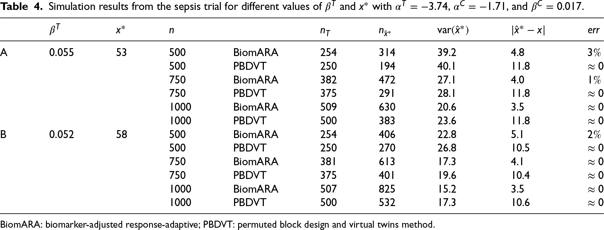
  The following simulation study is intended to mimic a clinical trial for patients with severe sepsis disease. The primary outcome is status (deceased or not) at 28 days after treatment. Based on this dataset, since age is found to be a predictive biomarker, the goal is to find the age above which the success probability of the treatment is higher than the success probability of the control. The values of the age of patients, ranging from 33 to 93 years, were sampled with replacement from the dataset available at https://biopharmnet.com/subgroup-analysis-software/ while patients’ responses were simulated across different experimental scenarios corresponding to different underlying truths about the predictive strength of the biomarker and, consequently, the threshold. Scenario A refers to ${\alpha }^T=-3.74$ , ${\alpha }^C=-1.71$ , ${\beta }^T=0.055$ , and ${\beta }^C=0.017$ , obtained by fitting a logistic model to the data: in this case, the true threshold is around 53 years. Scenario B takes into account ${\beta }_T=0.052$ (the corresponding threshold is 58 years). In this study, the BiomARA (with $ϵ=0.3$ ) is compared to a design strategy (Permuted Block Design and Virtual Twins method) which employs the PBD of size 4 for randomizing subjects and the Virtual Twins method ¹ as a subgroup identification method (implemented by the R package aVirtualTwins available on CRAN). For each scenario, Table 4 reports the average number of patients in the treatment group $n_T$ , the average number of patients with age greater than the estimated threshold $n_{{\hat{x}}^{*}}$ , the average $|{\hat{x}}^{*}-x|$ as a measure of bias and the percentage $err$ of simulations in which the trial ends up with a wrong conclusion. BiomARA shows smaller values of both the variance and the bias of the threshold, while the Virtual Twins method seems to suffer from a severe bias in this context. Finally, as previously discussed, $err$ is strongly sensitive to the sample size and to the closeness of the estimated threshold to the extremes of the support of the biomarker; however, due to the strong consistency of the MLEs, $err$ vanishes as $n$ increases regardless of the true threshold.

  Table 4.

  Simulation results from the sepsis trial for different values of ${\beta }^T$ and $x^{*}$ with ${\alpha }^T=-3.74$ , ${\alpha }^C=-1.71$ , and ${\beta }^C=0.017$ .

  

  	${\beta }^T$	$x^{*}$	$n$		$n_T$	$n_{{\hat{x}}^{*}}$	$\text{var}({\hat{x}}^{*})$	$|{\hat{x}}^{*}-x|$	$err$
  A	0.055	53	500	BiomARA	254	314	39.2	4.8	$3\mathrm{\%}$
  			500	PBDVT	250	194	40.1	11.8	$\approx 0$
  			750	BiomARA	382	472	27.1	4.0	$1\mathrm{\%}$
  			750	PBDVT	375	291	28.1	11.8	$\approx 0$
  			1000	BiomARA	509	630	20.6	3.5	$\approx 0$
  			1000	PBDVT	500	383	23.6	11.8	$\approx 0$
  B	0.052	58	500	BiomARA	254	406	22.8	5.1	$2\mathrm{\%}$
  			500	PBDVT	250	270	26.8	10.5	$\approx 0$
  			750	BiomARA	381	613	17.3	4.1	$\approx 0$
  			750	PBDVT	375	401	19.6	10.4	$\approx 0$
  			1000	BiomARA	507	825	15.2	3.5	$\approx 0$
  			1000	PBDVT	500	532	17.3	10.6	$\approx 0$

  BiomARA: biomarker-adjusted response-adaptive; PBDVT: permuted block design and virtual twins method.

6. Discussion

In this paper, we address the complex issue of patient enrollment restriction in the presence of a continuous predictive biomarker. Despite the advances in understanding disease mechanisms and the increasing discovery of biomarkers that affect patients’ responses to treatments, methodological results regarding continuous biomarker cutpoint identification and evaluation remain relatively few.

For binary response trials, in this work, we show that optimal designs for the estimation of the model parameters and the cutoff of a continuous predictive biomarker require multiple conditions to be satisfied, involving the patients’ biomarker values and the unknown model parameters. Such an optimal design can be implemented sequentially by adopting the new CARA procedure suggested in Section 4. An extensive simulation study, including a redesign of a clinical trial, highlights the advantages of the proposed approach.

Our research includes an analysis aimed at pointing out the pitfalls of the common and problematic approach of adopting (empirical) median-based biomarker cutoffs. From an ethical perspective, a fundamental requirement of a clinical trial is to ensure an overall benefit for the entire sample of enrolled patients and a widely used ethical criterion focuses on maximizing the percentage of patients who receive the best treatment. Given a prognostic biomarker (i.e. in the absence of treatment/covariate interactions), the relative performance of the treatments is the same for every subject’s profile; whereas, for predictive biomarkers (namely in the presence of treatment/covariate interactions), the superiority/inferiority of a given treatment, as well as their discrepancy, depends on the subject’s profiles. In this setting, discretizing continuous biomarkers is widely discouraged due to inferential and ethical repercussions (Polley and Dignam, ³ Zhang and Molinaro, ⁴ Bennette and Vickers, ²² and Royston et al. ²³ ). In contrast, our approach provides a cutoff identification methodology directly on a continuous scale which guarantees that more patients are assigned to the superior treatment (based on their biomarker), in line with the International Code of Medical Ethics, “a physician shall act in the patient’s best interest when providing medical care.” We strongly believe that the discretization of continuous biomarkers should be avoided and we encourage the researchers to abandon it.

The suggested procedure is suitable for early phase studies as it is aimed at guiding future treatment decisions for individual patients. It is worth mentioning that the approach proposed in this paper can be applied to any continuous biomarker distribution, provided that widely satisfied assumptions hold.

Some potential directions for future research have been identified. For instance, extending our approach by considering the generalized linear model family would certainly expand its applicability to a broader spectrum of clinical trial scenarios. In addition, we intend to extend our procedure to accommodate more than two treatments. Lastly, yet importantly, incorporating multiple biomarkers could make the identification of the target population more accurate.