
Abstract
Instrumental variables (IVs) methods have recently gained popularity since, under certain assumptions, they may yield consistent causal effect estimators in the presence of unmeasured confounding. Existing simulation studies that evaluate the performance of IV approaches for time-to-event outcomes tend to consider either an additive or a multiplicative data-generating mechanism (DGM) and have been limited to an exponential constant baseline hazard model. In particular, the relative merits of additive versus multiplicative IV models have not been fully explored. All IV methods produce less biased estimators than naïve estimators that ignore unmeasured confounding, unless the IV is very weak and there is very little unmeasured confounding. However, the mean squared error of IV estimators may be higher than that of the naïve, biased but more stable estimators, especially when the IV is weak, the sample size is small to moderate, and the unmeasured confounding is strong. In addition, the sensitivity of IV methods to departures from their assumed DGMs differ substantially. Additive IV methods yield clearly biased effect estimators under a multiplicative DGM whereas multiplicative approaches appear less sensitive. All can be extremely variable. We would recommend that survival probabilities should always be reported alongside the relevant hazard contrasts as these can be more reliable and circumvent some of the known issues with causal interpretation of hazard contrasts. In summary, both additive IV and Cox IV methods can perform well in some circumstances but an awareness of their limitations is required in analyses of real data where the true underlying DGM is unknown.
Introduction
Randomised controlled trials (RCTs) are getting shorter and more streamlined as regulatory bodies, such as the Food and Drug Administration and European Medicines Agency, look to speed up access to innovative health care. Policy makers need to conduct heath technology assessments to determine whether treatments are actually cost-effective before approving them for clinical practice. The increasing availability of very large data resources, such as electronic health record (EHR) data, means that we now have vast amounts of observational data that include information on outcomes that are not always possible to evaluate in a randomised trial. For example, most trials do not run for long enough to observe data on overall survival and use progression-free survival as a surrogate endpoint. Even though regulators and licensing bodies will approve a treatment based on its performance with regard to progression-free survival, the longer follow-up periods that are found in cancer registry or EHR data are required to support cost-effectiveness analyses. Due to the limited availability of RCT evidence, there is hence heightened interest in reliable methods for treatment effect estimation from observational data with a view to supplementing, or possibly even to replacing, evidence from RCTs. 1 Observational effect estimators can be biased in the presence of unmeasured confounding and while there are many methods that try to alleviate such bias, their relative performance is unclear. 2 Importantly, if we want to replace or supplement evidence from an RCT, we need methods for observational data that provide reliable and valid results under plausible assumptions.
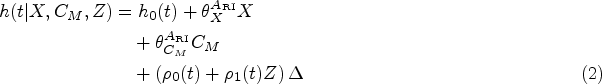
Unlike other adjustment methods, such as adjustment based on the propensity score, instrumental variable (IV) approaches can consistently estimate causal effects in the presence of unmeasured confounding provided certain conditions are satisfied. For exposure
Note that only the first of these can be verified empirically as the others involve the unmeasured confounding
The Cox-proportional hazards model, which assumes multiplicative covariate effects on the hazard scale, is the most widely used model for time-to-event data but there has been limited development of IV methods for this model until recently.14–17 A two-stage approach, analogous to that used for continuous outcomes, is easy to implement and often used in practice but is not guaranteed to be consistent for a causal effect. 18 The structural Cox model, 17 on the other hand, targets a particular causal hazard ratio: the causal effect of treatment among treated subjects. Alternatively, additive hazards IV models have been proposed for time-to-event data since the hazard difference is a collapsible effect measure under the additive hazard model.7,19–21 In particular, the two-stage residual inclusion (2SRI) approach, also known as the control function approach, consistently estimates the marginal causal hazard difference when the exposure is binary. 7 Both additive hazards and Cox IV methods have been applied to observational data, for example, Desai et al. 22 used an additive control function approach to assess the effect of osteoporosis medication use on subsequent fractures whereas Guo et al. 23 used a two-stage Cox IV model to consider the effect of body mass index (BMI) on breast cancer survival in a Mendelian randomisation (MR) study. In practice, the Cox model tends to be more widely used than the additive hazards model and remains the standard analysis model for clinical trials. This may be due to the lack of restriction on the additive hazards model to ensure a non-negative hazard and hence valid survival probabilities. 24 Yet, if we consider the RCT as the gold standard, a method that identifies a marginal causal effect might seem preferable. It is hence important to assess the sensitivity of these additive IV models to departures from the additivity of covariate effects.
Previous simulation studies to compare IV approaches to time-to-event analyses either focus on the relative performance of Cox IV methods where the data are generated with multiplicative covariate effects, that is, under a multiplicative data-generating mechanism (DGM),16–18 or on the performance of additive IV methods under an additive DGM.19,20 Recently, Cho et al. 25 assessed the performance of both additive and Cox IV methods but under the relevant DGM for each method. These studies also tended to focus on an exponential model for the baseline hazard which remains constant over time.
Here, we present an extensive simulation study that compares these different IV approaches in as unprejudiced a way as possible using additive-hazard and multiplicative-hazard DGMs alongside different baseline hazard models. We also consider much larger sample sizes than used in other studies reflecting the large samples that we would expect from EHR data. In addition to targeting causal contrasts on different scales, for example, hazard differences versus hazard ratios, some of the methods target conditional, or sub-group specific, rather than marginal, or population, parameters. While our primary interest is in the consistent estimation of a marginal causal parameter comparing treatment versus control, as targeted by an RCT, we also consider how each estimator performs with regard to its target estimand on the relevant scale, regardless of the DGM. The additive IV methods are always assessed with regard to how well they recover the relevant true hazard difference and the Cox IV method estimates are always compared with the relevant true hazard ratio. Despite their fundamental differences, all these models target survival probability predictions so we also consider survival probabilities to compare the different models.
The paper is structured as follows. The first section describes the analysis models to be evaluated, the simulation of survival times using exponential and Weibull baseline hazard models and the design of the simulation study. We discuss how to make the different scenarios comparable for additive and multiplicative DGMs and how to obtain the true estimands for each scenario. The results of the study are then presented. We then apply the methods to a study of the effect of statin treatment on the time-to-developing Type 2 diabetes and we conclude with a discussion of our findings where we make some practical recommendations and propose potential avenues for further work.
In this section, we present the analysis models to be compared and their target estimands. We then describe how we simulate observational time-to-event data and how we endeavour to make the comparison between multiplicative and additive models as fair as possible over a wide range of scenarios. We then show how we evaluate the relevant estimands for each scenario and finally describe the simulation study itself.
Analysis methods
For survival times Additive hazards IV methods.
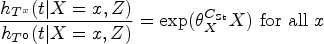
Cox IV methods.
An adjusted additive hazards model, also known as a semi-parametric additive hazards model26,27:

Naïve Cox proportional hazards regression (
)
An adjusted Cox proportional hazards model:

Two-stage additive IV method (
)
This approach is inspired by two-stage methods for linear no-interaction models. The first stage is a logistic regression of


This approach takes the estimated residuals,
This method is analogous to the two-stage additive IV method above. The first stage fits a logistic regression of

Structural Cox IV method (
)
Martinussen et al.
17
propose an approach to estimate the causal effect of treatment on the treated based on a structural Cox model:
Under the IV assumptions and the above structural model, an estimator is obtained as a solution of

Table 1 provides a summary of the analysis methods to be compared together with the causal contrasts they target and their required assumptions.
Target parameters and model assumptions for different analysis methods. All IV methods require no interaction or effect modification by
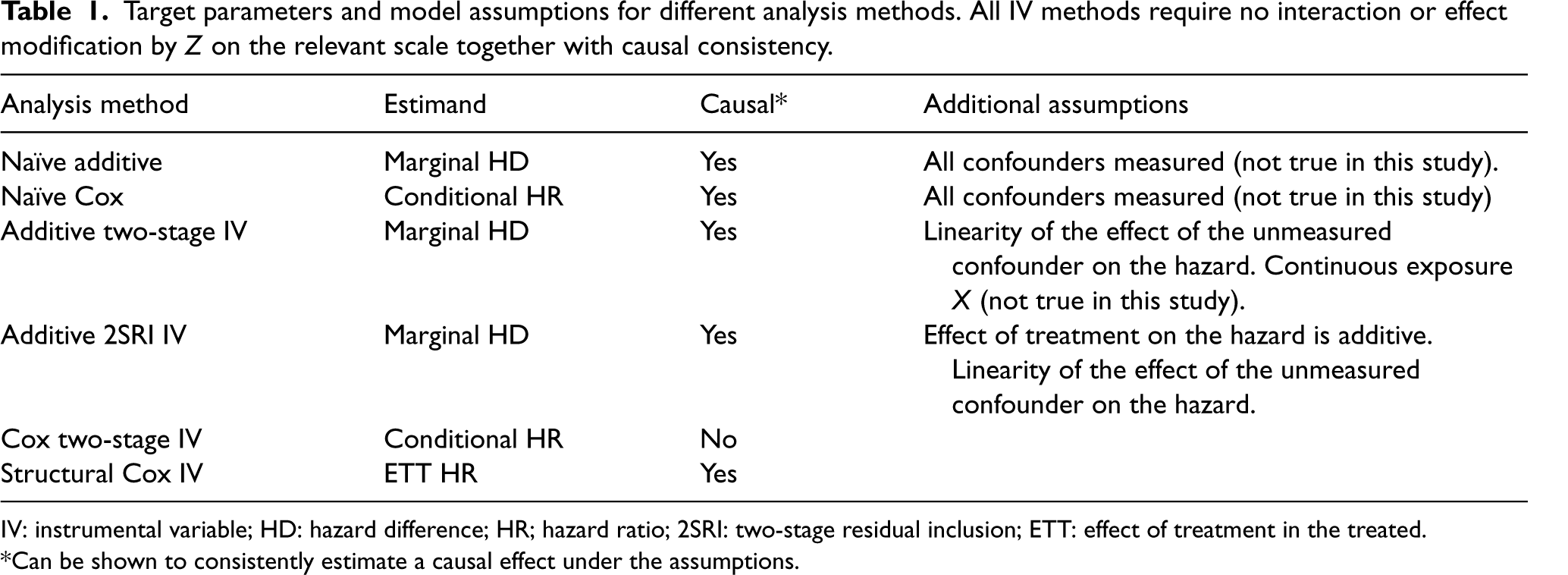
IV: instrumental variable; HD: hazard difference; HR; hazard ratio; 2SRI: two-stage residual inclusion; ETT: effect of treatment in the treated.
*Can be shown to consistently estimate a causal effect under the assumptions.
A binary instrumental variable 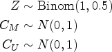

Survival times
Hazard and survival functions under different data-generating mechanisms (DGMs) and parametric distributions where
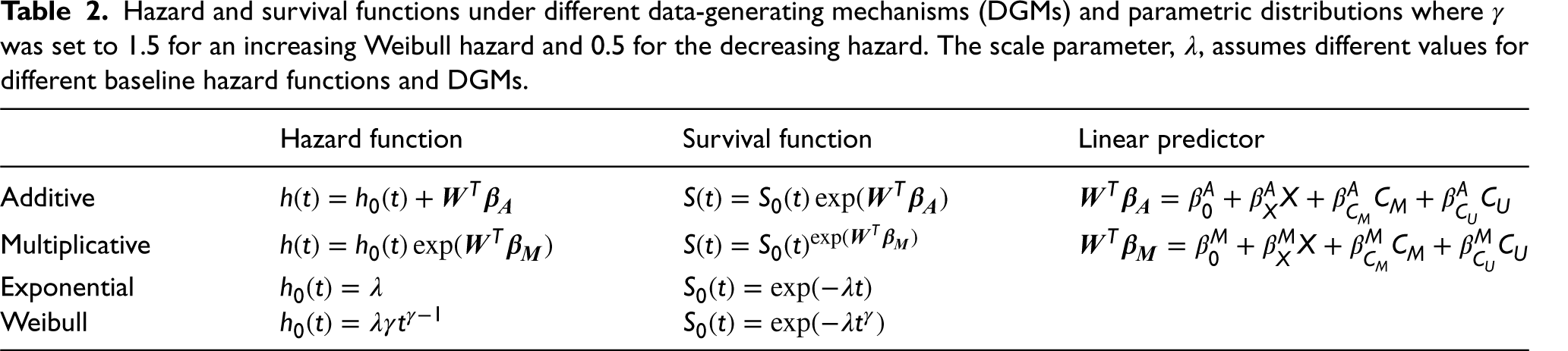
The coefficients
Generating similar survival curves under additive and multiplicative DGMs was a challenge, particularly so for a Weibull baseline and multiplicative DGM as the shape of the survival curves, in that case, is especially difficult to capture using additive hazard models. We started with the multiplicative DGM and then sought corresponding values for the additive DGM. The specified coefficients for each scenario under a multiplicative DGM (
Coefficient values used to simulate data in the different simulation scenarios. The last column gives the term that will be used to refer to each corresponding scenario.
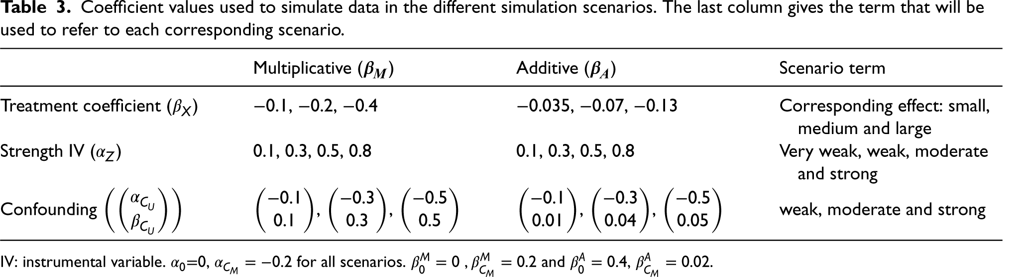
IV: instrumental variable.
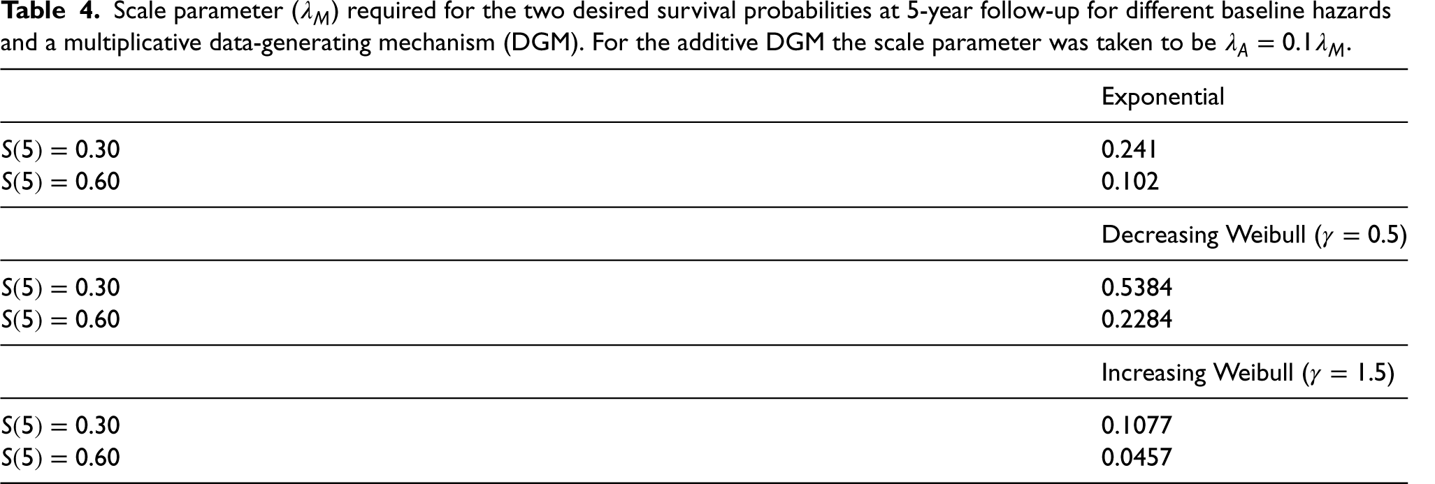
Scale parameter (
In total,
The motivation behind trying to match survival curves is so that they reflect plausible survival proportions observed in real data examples, whatever the underlying (unknown) DGM. For example, in the clinical practice research database (CPRD) analysis, the observed survival at the end of follow-up is above
The F-statistic from a linear model of the IV on treatment is commonly used as a measure of the strength of the instrument. An F-statistic over
As noted above (Table 1), different analysis models target different causal effects (i.e. marginal, conditional on
Causal hazard difference:


Regardless of the underlying DGM, the true causal contrast can be evaluated in terms of a hazard ratio and hazard difference for each simulation scenario allowing for bias in the multiplicative Cox methods to be assessed under a truly additive DGM and bias in the additive hazards methods to be assessed under a truly multiplicative DGM. The actual value of the true causal contrast will depend on several factors such as the distribution of the baseline hazard, strength of confounding, treatment coefficient and whether the DGM is additive or multiplicative.
The true causal hazard ratios, hazard differences and true survival probabilities for each treatment arm could be approximated using numerical integration but we will instead employ a Monte Carlo (MC) approach analogous to that applied elsewhere.
28
In our case, we will generate data for each of our we draw 2,000,000 covariates we then randomly allocate subjects to treatment survival times, unadjusted Cox and unadjusted additive hazards regression models are fitted to
Since there is no guarantee that the true hazard ratio or hazard difference is constant over time in our scenarios, Step
Simulation study
The analysis methods were compared on simulated datasets of size 2000, 10,000 and 100,000 for each of our 432 scenarios. There were 1000 replicated datasets for each scenario except for the case of the largest sample size (100,000) where 200 datasets were considered. Our primary focus is on the marginal causal contrast, the natural target of an RCT, but we also consider conditional or subgroup effects when relevant. IV estimators are known to be more variable than conventional estimators so we are particularly interested in the bias. The following outcome measures were recorded for each analysis model Estimated treatment effect: Standard deviation of the estimates across the replicated datasets (MC standard error) MC bias: Mean squared error (MSE): Relative bias: Coverage: Percentage of default Power: Percentage of
where
Computing
Data simulation and analyses were conducted using statistical software
Results
The results are split into two sections: the results for the treatment effect estimates, and the results for the survival probability predictions. We will focus on the results for the medium sample size (
Treatment effect estimates
We begin with the estimation of the marginal population causal effect, which is the target of an RCT, after
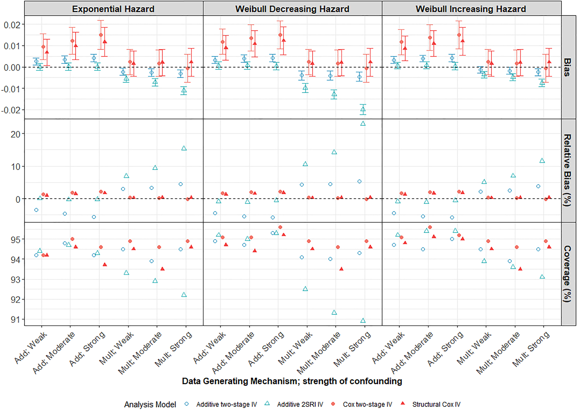
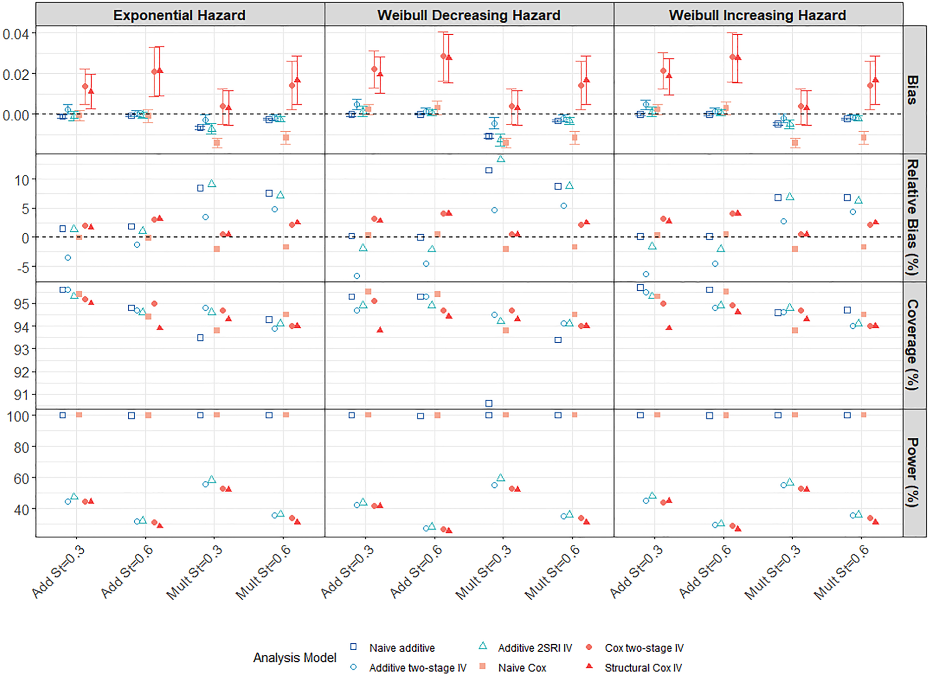
Performance of IV methods across different confounding strengths in a scenario with a large treatment effect, moderate IV and low survival probability
Both Cox and additive naïve methods (Supplemental Figure D1) were, not unexpectedly, very biased in the presence of moderate or strong unmeasured confounding and much more biased than any of the IV methods. The bias increases with confounding strength up to a relative bias of over
Mis-specification of DGM
The 2SRI additive IV method clearly outperforms the two-stage model under an additive DGM, even with strong confounding, presumably reflecting the fact that the two-stage model assumptions are not satisfied for a binary exposure. However, it is more sensitive to misspecification of the DGM and estimates are more biased than those from the two-stage additive IV model when the DGM is multiplicative. Both the two-stage and structural Cox IV models exhibited low levels of MC bias for the marginal hazard ratio under a multiplicative DGM. Importantly, the Cox IV models also seem to be less affected by misspecification of the DGM than the additive models. Notably, the structural Cox IV method which targets the ETT, appeared to be only slightly biased for the marginal hazard ratio (with a relative bias of
Variability in IV models
All IV estimates were variable with large MC standard errors observed for all strengths of IV and confounding. Thus, for a large proportion of the simulated datasets, the estimated treatment effect can be quite different from the truth. The difference in variability between the nai
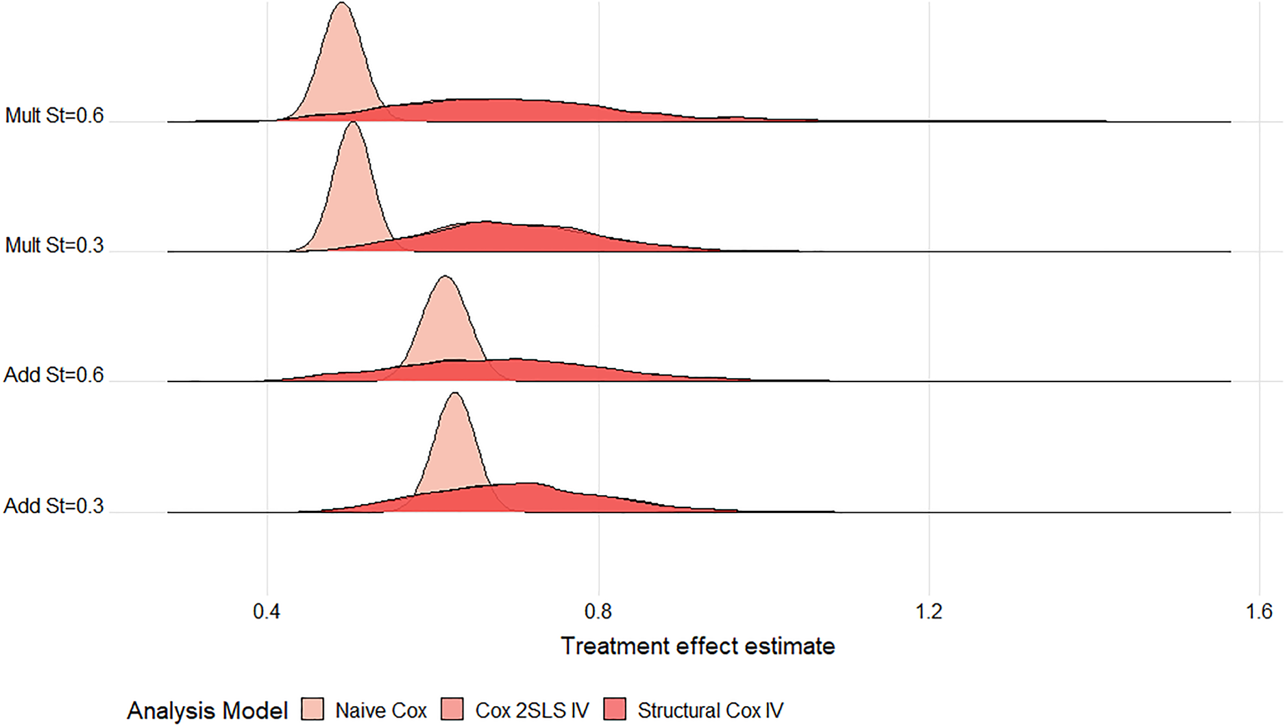
Ridgeline plot of treatment effect estimates from the Cox models across
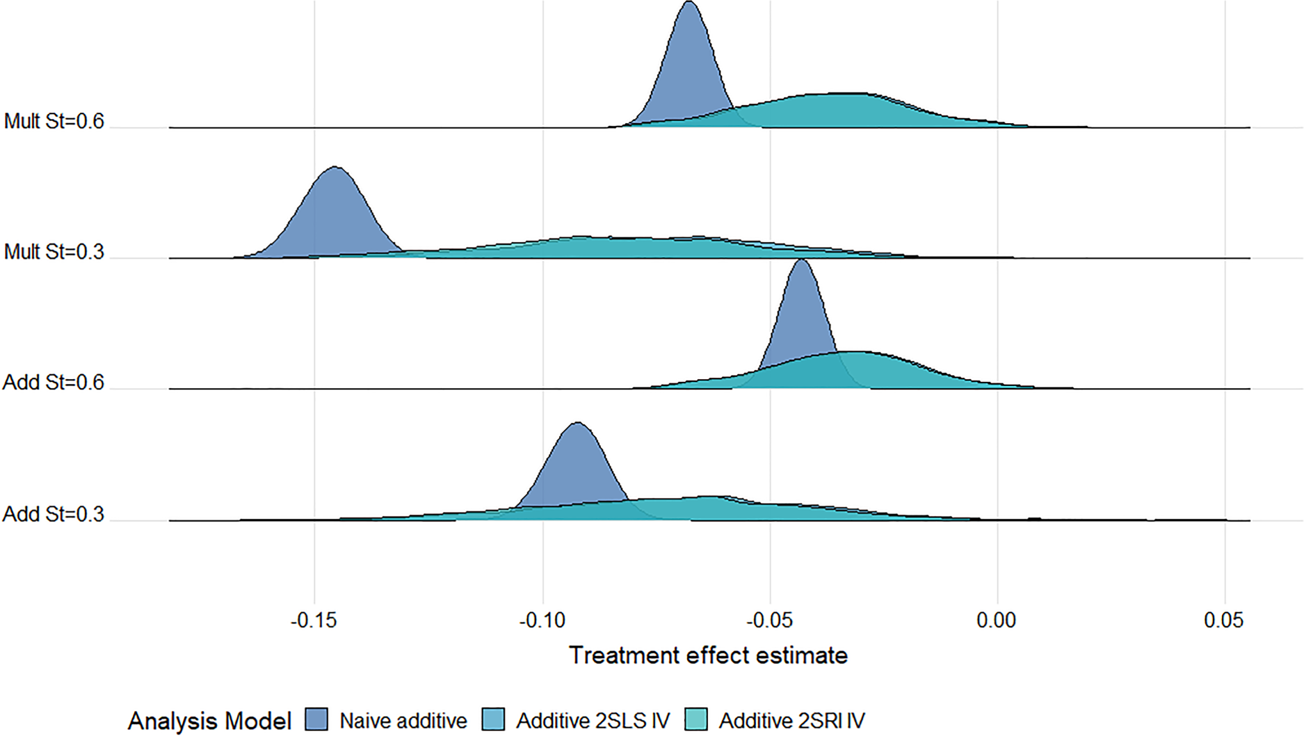
Ridgeline plot of treatment effect estimates from the additive models across
Under both multiplicative and additive DGMs, the bias and variability (MC standard error (SE)) of IV methods reduce as the strength of IV increases from weak to strong (Figure 4). When the IV is very weak (
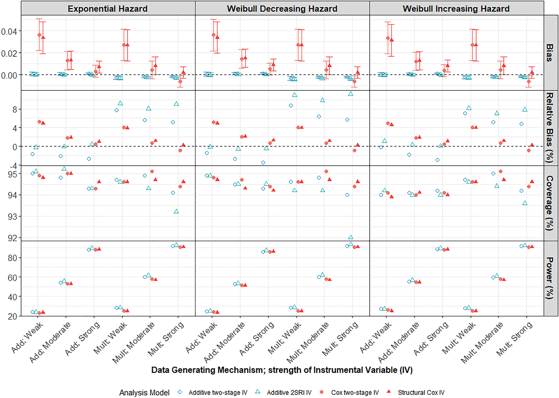
Performance of IV methods across different IV strengths compared to the marginal true parameter at 5 years follow-up. Scenario with large treatment effect, moderate confounding and low survival probability
Small sample bias was evident for our smallest sample size (
Performance of all methods compared to the true marginal effect at 5 years follow-up in a scenario with large treatment effect, weak confounding and strong IV (
Up to now, the discussion has focused on the marginal causal contrast which is the natural target of an RCT. However, the structural Cox IV method targets the ETT and the two-stage Cox IV model targets a conditional effect so we also considered how well these other causal contrasts were estimated. Note that the marginal and conditional/ETT causal hazard differences will not necessarily be identical under a multiplicative DGM.
The Cox methods appear to be generally more biased for their target estimands than for the marginal effect. However, as noted above, our simulation does not guarantee that there is no effect modification by
Effect estimates over time
Finally, we also considered estimates obtained after each year
Survival probability predictions
Additive DGM
Under an additive DGM, the survival probability predictions for the 2SRI additive IV and Cox IV methods exhibit very little bias across all strengths of confounding. This can be seen in the left-hand panel of Figure 6 for a decreasing Weibull baseline hazard where the average difference between predicted and true probabilities is very close to zero at all years of follow-up for the untreated (
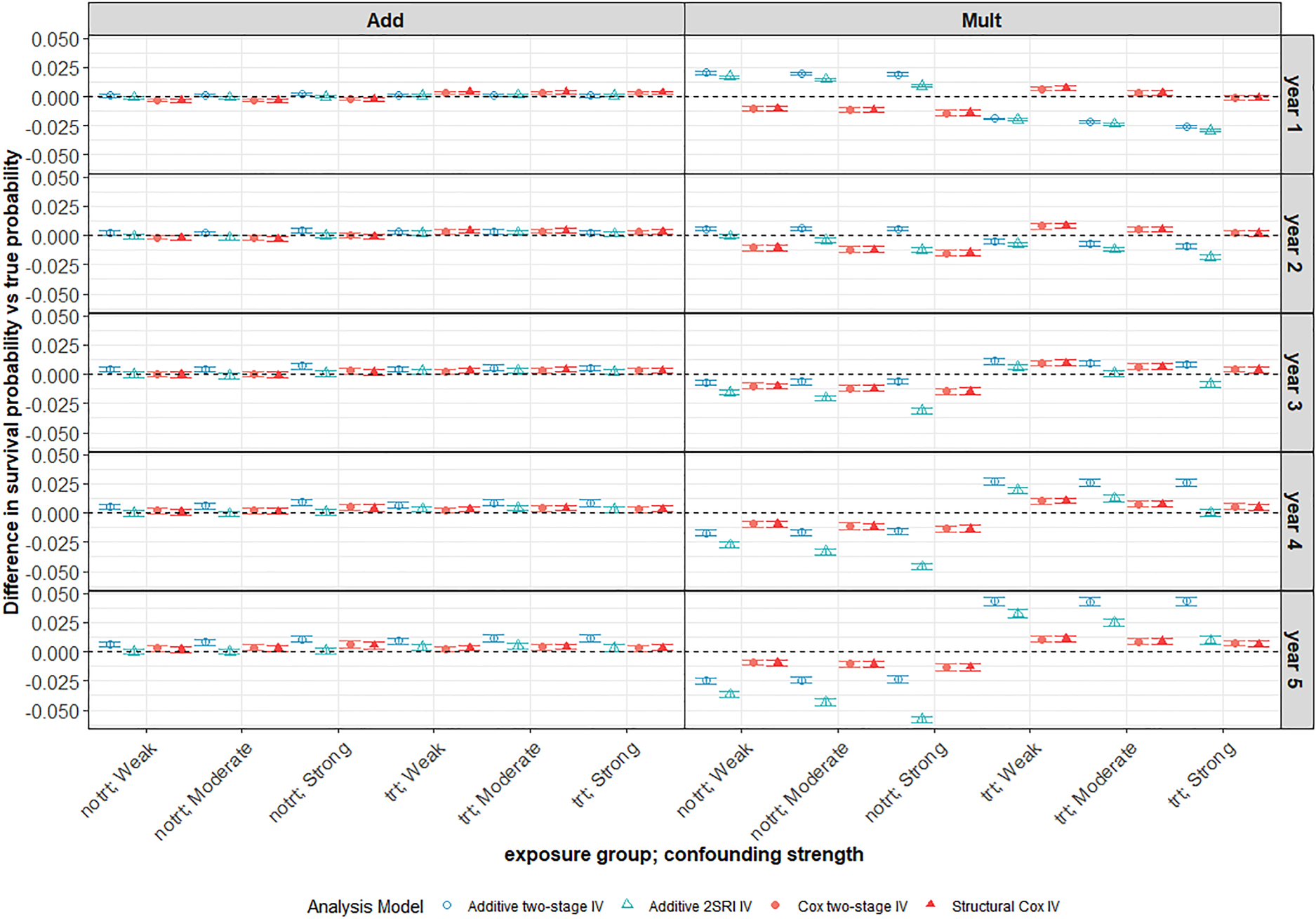
Average difference between survival probability predictions and the true marginal survival probabilities for different confounding strengths. Scenario with large treatment effect and weak IV under a decreasing Weibull baseline hazard with low 5-year survival probability (
However, when the data are generated under a multiplicative DGM for a decreasing Weibull baseline (Figure 6 right-hand panel), the survival probability predictions appear to be biased for all IV methods and more so for the additive models. The Cox IV methods slightly under-predict survival in the untreated group and slightly over-predict in the treated group with average bias increasing slightly with the year of follow-up, but never to much more than
Impact of confounding
For all IV methods, bias in survival predictions increases slightly with confounding in the untreated arm but tends to decrease with increased confounding in the treated arm. As expected, both naïve methods give worse survival predictions in the presence of unmeasured confounding with bias increasing for stronger confounding (Figure 7). Predictions are generally worse for all methods under a multiplicative DGM. There is much more variability in survival probability predictions from all IV methods than from the corresponding naïve methods. Again, the variability problem does not go away with increased sample size, as can be seen in the ridgeline plot of Figure 8 for a scenario with 100,000 observations, although it is less extreme than for
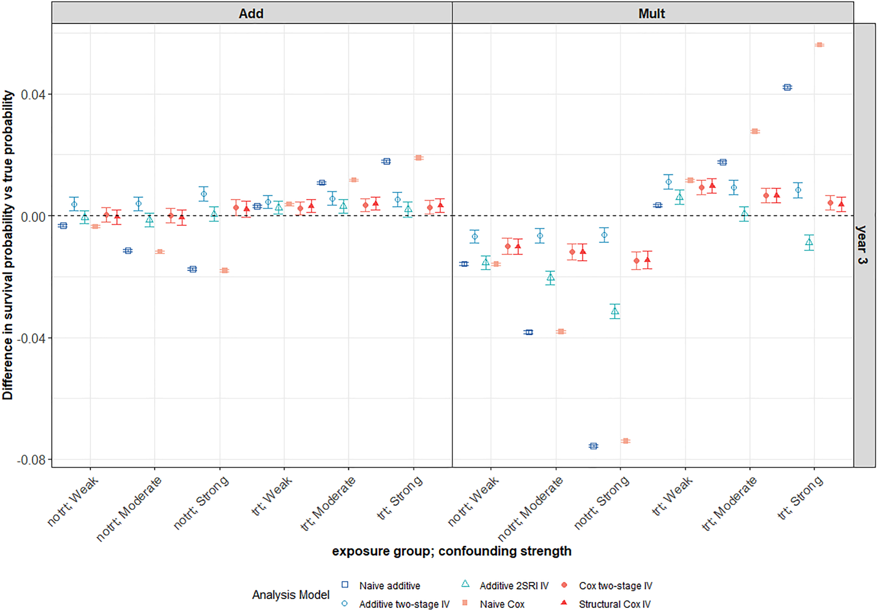
This plot focuses on the third year of follow-up for the same scenario as in Figure 6. Average differences between survival probability predictions and the true marginal survival probabilities for different confounding strengths. The survival predictions for a 3-year follow-up are plotted for both the naïve and IV methods. The scenario with large treatment effect and weak IV under a decreasing Weibull baseline hazard with
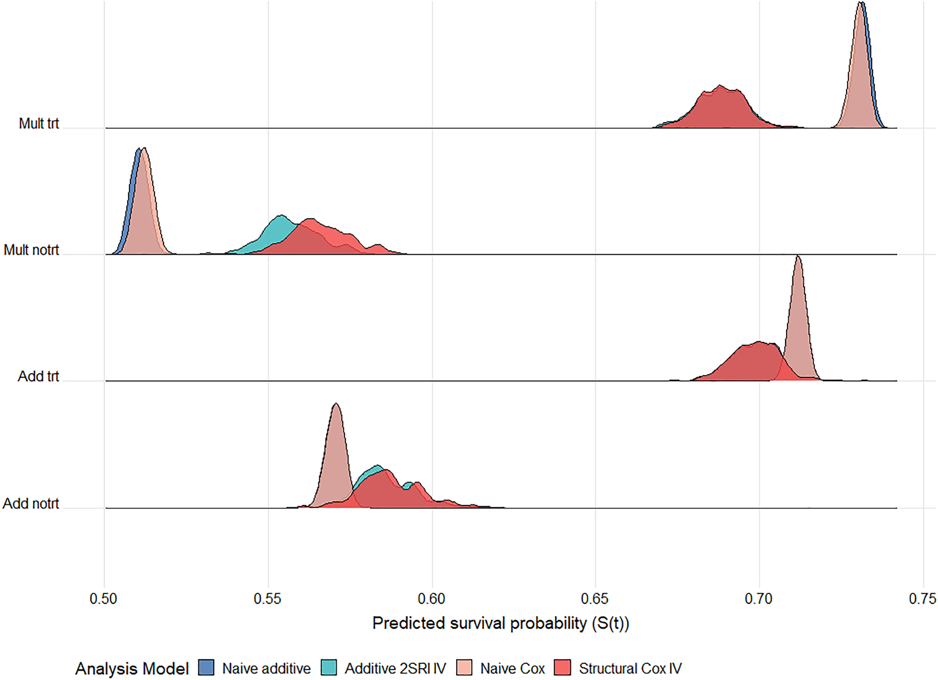
Ridgeline plot of survival probability predictions at 5 years follow up across
Overall, the Cox IV methods yield survival probability predictions with very little bias regardless of the underlying DGM. The 2SRI additive IV method performs best under an additive DGM but is sensitive to the DGM and to the baseline hazard function. As noted earlier, the shape of the survival curves for a Weibull hazard function and multiplicative DGM is difficult to capture using additive hazard models in our scenarios. Performance is poor for all methods and all baseline hazard functions when the IV is very weak (
Statins have been found to reduce the risk of major cardiovascular events by lowering blood cholesterol. 40 However, there are concerns that the use of statins can increase the risk of patients developing Type 2 diabetes mellitus (T2DM).41,42 The health problems and complications associated with T2DM may affect the benefit–risk ratio of prescribing statins to people with low risk of cardiovascular disease. A previous study found the rate of developing T2DM to be 57% (95% CI [54%, 59%]) higher in patients on statins compared to those not on statins. 43 These results may be affected by unmeasured confounding factors. We conduct a similar analysis but using IV methods to obtain estimates of the effect of statins on the development of T2DM. 44
Study design
This is an observational population-based retrospective cohort study of
Instrumental variable (IV)
A potential instrument for use in this analysis is a cardiovascular disease (CVD) risk score since patients with a higher CVD risk are more likely to be prescribed statins. The QRISK score
45
estimates cardiovascular risk with patients classified as being clinically at high risk if their 10-year cardiovascular risk is >20%. Here, CVD risk is dichotomised as high risk (
In order to assess the validity of the CVD risk score as an instrument, the predictors for the CVD score need to be compared with predictors of the outcome of interest, T2DM. The factors that are associated with T2DM are taken from the diabetes risk tool.46,47 Plausible associations between the different variables, the instrument
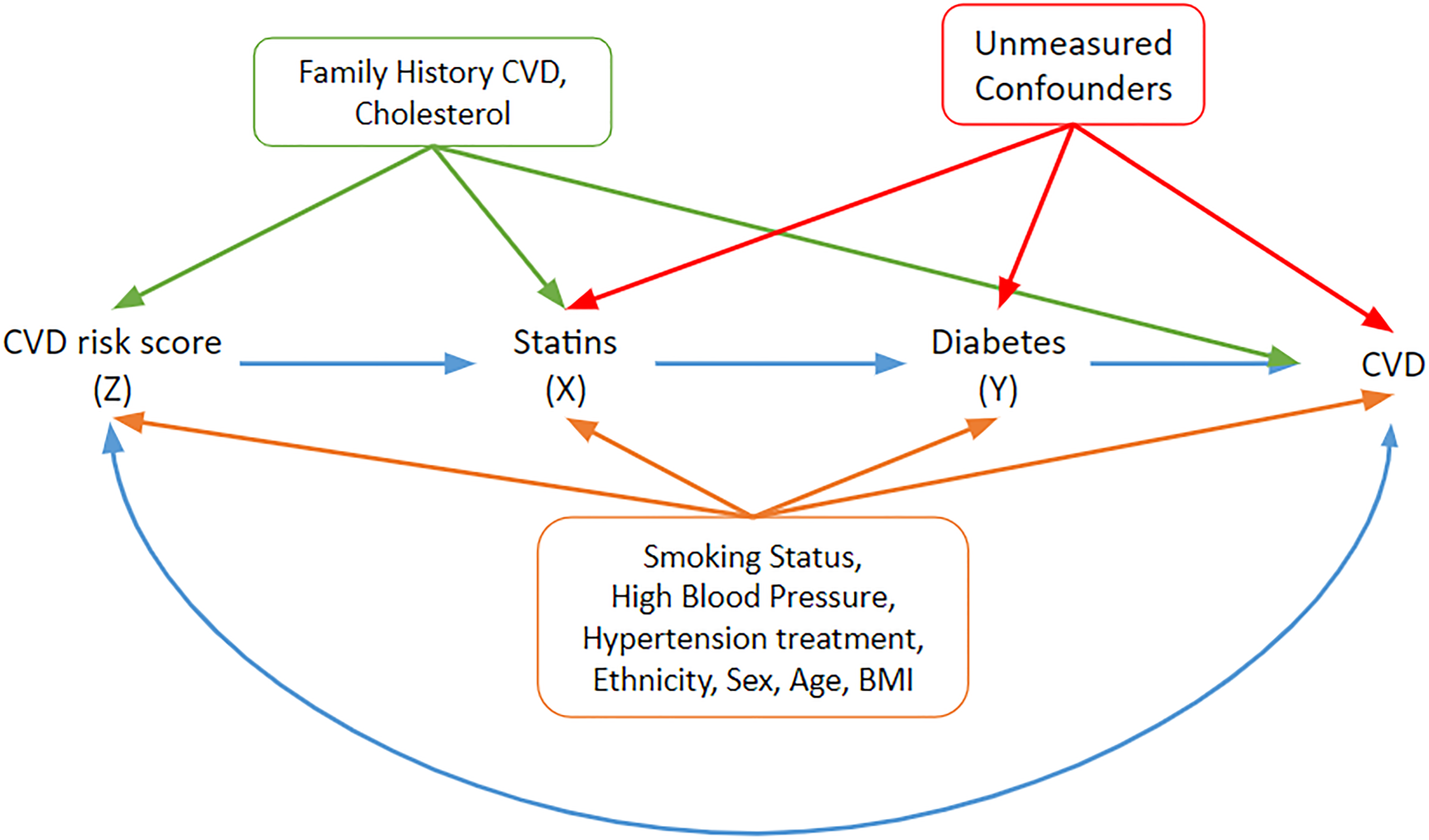
A DAG under which the graphical IV assumptions hold and under which the statin effect estimates may be interpreted as structural/causal. Relevant covariates and their potential pathways are included. The orange covariates need to be adjusted to block paths from the instrument to the outcome of interest (T2DM). The blue double-headed path represents other common causes of risk score and CVD that do not have to be accounted for. IV: instrumental variable; DAG: directed acyclic graph; CVD: cardiovascular disease; T2DM: Type 2 diabetes mellitus.
Family history of CVD and cholesterol are associated with the instrument
Naïve analyses
Naïve additive and Cox regression models were initially fitted to the data. These models are adjusted for the main covariates: hypertension, smoking, ethnicity and BMI, which were associated with CVD risk (Figure 9) and are given in Supplemental Table E1 in Supplemental Appendix E. The naïve Cox model found there was a
Similar trends were observed in the naïve additive hazards model. Exposed patients had an additional hazard of
IV analyses
In order to assess the strength of the CVD risk score as an instrument, logistic and linear regression models of exposure (statin use) on an instrument, adjusted for the measured confounders identified in Figure 9 were fitted. The logistic regression model showed that patients with high 10-year CVD risk had
Alternatively, as seen in the simulation study, the probability of exposure for the different IV groups can be compared to assess the strength of the instrumental variable. In this study,
The results for the different IV models are presented in Supplemental Table E3 in Supplemental Appendix E. Both Cox IV models suggested that exposure had a causal effect on the development of T2DM but the magnitude of the effect varied depending on the model chosen. The structural Cox model found a causal effect of exposure with a
A 2SRI additive IV model was also fitted to the data and yielded an additional hazard of
Survival predictions
The survival probability predictions, which represent the probability of being diabetes free, are shown in Figure 10 for the different analysis models.
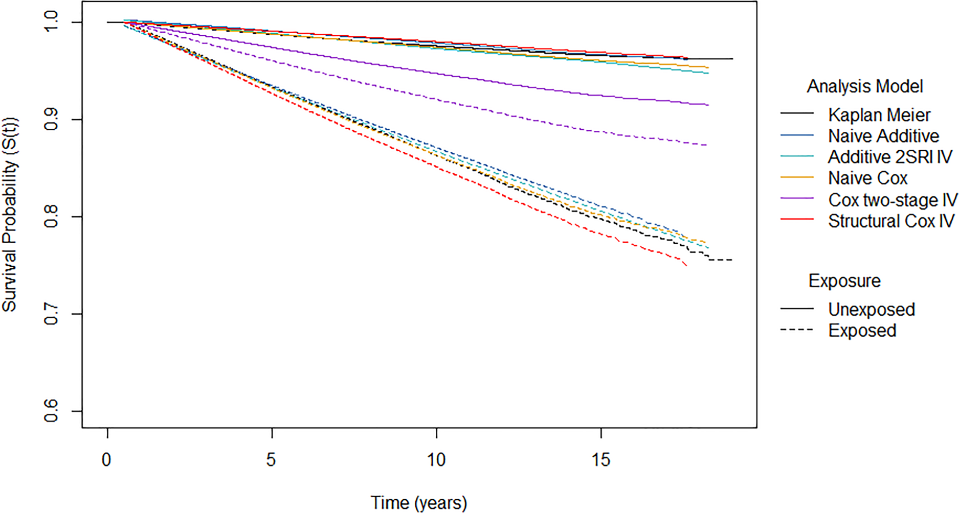
Survival probability predictions from different analysis models by exposure group. Note the
The naïve Cox, naïve additive and 2SRI additive IV models yield similar standardised survival predictions in both exposure arms. In the unexposed group, the proportion of patients that were diabetes free after 10 years of follow-up was estimated to be 97.4% for the naïve Cox model, 97.8% for the naïve additive model and 97.2% for the 2SRI additive IV model. In comparison, a lower proportion of patients were estimated to be diabetes free after 10 years of follow-up in the exposed arm: 86.3% for the naïve Cox model, 87.1% for the naïve additive model and 86.7% for the 2SRI additive IV model. This suggests that the probability of developing diabetes after 10 years is 10% higher if everyone were exposed compared to if nobody were exposed. It should be noted that we only obtained predictions at five time points from the 2SRI additive IV model due to computational issues.
The two-stage Cox IV model has much lower survival under no exposure (94.7%) and much higher survival under exposure (92.1%) compared to the other models. This reflects the much smaller hazard ratio that was obtained from the two-stage Cox IV model. The structural Cox IV model obtains similar predictions under no exposure as the other analysis models with a 10-year survival of 97.9%. However, lower survival is predicted under exposure compared to other analysis models with a 10-year survival of around 85.1%. This suggests that the probability of developing diabetes under exposure to statins is 13% higher than if the same patients had not been exposed.
All models found that statin exposure increased the risk of T2DM with none of the confidence intervals covering the relevant null effect. Not surprisingly, however, the magnitude of the effect was dependent on the analysis model used. For the most part, the IV models resulted in a larger effect of exposure on T2DM than the naïve models. Only the two-stage Cox IV model delivered a smaller exposure effect although this model is not guaranteed to target a causal estimand. The additive IV models exhibited more uncertainty about their effect estimate compared to the naïve additive regression models, as can be seen from the standard errors reported in Supplemental Table E3 in Supplemental Appendix E. This increased uncertainty was also reflected in the increased MC errors in the simulation study. The uncertainty under the structural Cox model was much more comparable to that of the naïve Cox model for this dataset whereas it was much more variable than the naïve model in the simulation study. The findings support the hypothesis of a positive causal effect of statin use on the development of T2DM but we should be wary about drawing firm conclusions about the actual size of this effect.
RCTs remain the preferred choice for causal treatment effect estimation because randomisation ensures that confounding factors, measured or unmeasured, do not affect the estimates. However, some clinical outcomes of interest cannot be observed in an RCT and estimates from observational data are required. It is important to verify how reliable such estimates are likely to be. Standard adjustment approaches can be misleading because they fail to account for unmeasured confounders. IV methods can account for these and produce unbiased causal effect estimates in some situations but they rely on strong assumptions that cannot always be verified from the data. IV estimators, such as the well-known two-stage least squares (2SLS) estimator, are well developed for continuous outcomes assuming a linear additive model with no interactions but application is more problematic for non-linear models.
Our focus is on treatment effect estimation for survival, or time-to-event outcomes for a binary treatment indicator. In this study, we compared additive hazards and multiplicative hazards (Cox) IV methods, the relative merits of which, to our knowledge, have not been fully considered before. The performance of the methods was evaluated on a wide range of scenarios where the strength of confounding, strength of instrument, size of treatment effect and baseline hazard distribution were varied. Data were simulated under both additive and multiplicative DGMs so that the methods could be compared when their assumptions about the underlying DGM do and do not, hold. A truly fair comparison is difficult as these are fundamentally different models, operating under different model assumptions, different scales and targeting different causal estimands. Our approach was to generate additive and multiplicative DGMs matched on
Despite their differences, it is natural in the context of survival analysis to expect that all the methods should predict survival, so we also compared their predicted survival probabilities with the true probabilities. Most IV analyses are designed to estimate causal hazard contrasts and do not consider survival probabilities. However, reporting survival probabilities, alongside hazard contrasts, can aid interpretation and avoid some of the problems with causal inferences based on hazard function estimates and the inherent selection bias induced by conditioning on prior survival.21,28,50–59 We note that these predictions are not guaranteed to be causal probability estimates since the Breslow estimator, required to obtain predictions from the Cox IV methods, for example, only accounts for the measured confounders.
Under an additive DGM, the additive 2SRI, or control function, IV estimator performed well, even when survival was low, but was extremely sensitive to misspecification of additivity. Performance was particularly poor for a multiplicative DGM with a Weibull baseline hazard function where the shape of the survival curves is difficult to capture using additive hazard models. The two-stage additive IV model estimator was always biased, presumably reflecting the fact that the two-stage model assumptions are not compatible with a binary exposure. The Cox IV methods, on the other hand, were not quite as sensitive to departures from their assumption of multiplicative covariate effects with the structural Cox method generally out-performing the two-stage Cox IV method – provided the IV was sufficiently strong. The structural Cox IV method also targets a causal parameter, the effect of ETT. The two-stage Cox method does not target a causal parameter, but its performance was not much worse than that of the structural Cox method in many cases, and it is very simple to fit. A very recent paper
60
proposes an alternative IV estimator of the marginal causal hazard ratio, which is consistent under the assumptions of a marginal structural Cox model with an additional no-effect modification assumption in the first stage regression model. We have now tested this method on our simulated scenarios and found that it performed very similarly to the structural Cox IV method in these cases. However, all IV methods exhibited great variability across the simulations in both effect estimates and survival predictions, and this variability was still quite apparent in the largest sample size we considered (
We verified that the IV should not be very weak, even with weak confounding where an IV approach is not really required. Again, performance could actually be worse than that of the corresponding naïve methods which ignore the problem of unmeasured confounding that we aim to address. There is a limit on how strong an IV can be when the unmeasured confounding is strong and thus we need to account for weak IVs in practice.
61
We also require very large sample sizes. This is consistent with known issues for the 2SLS estimator when the IV is weak and the sample small.
36
However, what constitutes ‘small’ depends on the distributions of outcome, exposure and IV and for our time-to-event outcomes we found that
There are a few limitations and practical issues to be considered. This simulation only applied routine censoring at the end of the follow-up. Previous studies generated censoring times that follow an exponential distribution depending, in some scenarios, on the measured covariates.19,20,25 A more complex censoring mechanism would most likely increase bias in the effect estimators, especially if censoring were to depend on the exposure.
19
We also generated two simple normally distributed covariates with no interactions between the covariates and treatment. Clearly, more complex covariate patterns with interactions and time-dependent effects would be more realistic. In our CPRD application, for example, it is quite likely that there would be time-dependent effects. However, our aim was to compare the performance of IV methods in settings matched on
Our study focused on scenarios where there is a valid IV. No IV method can be relied upon to perform well if the IV is invalid.39,62,63 However, finding an IV is not always easy and finding a suitably strong one is even less so. In observational situations, non-randomised instruments such as our CVD risk score have to be justified based on the available background knowledge. Background information can, of course, change over time so it should be reviewed for every new analysis. In MR applications, the genetic variants used as IVs can often be validated convincingly if there is good biological information available. Genetic IVs are typically weak. However, it is sometimes possible to combine multiple IVs into genetic risk or allele scores which can yield a stronger IV provided all the individual IVs are themselves valid.64–66 There is often very little choice for IVs in health services research applications where measures such as physicians’ prescribing preference, calendar time or distance to facility are typically used.67,68 They may or may not be strong and are difficult, if not impossible, to combine.
In several scenarios, the additive hazards IV methods gave survival predictions outside the 0 to 1 range under both additive and multiplicative DGMs (see Supplemental Figure D18 in Supplemental Appendix D for an example). This happens when the estimates of the hazard obtained for some of the event times are negative. When first proposing the model, Aalen
24
highlighted that the hazard is not restricted to non-negative values and consequently implausible survival functions can arise.
27
Our data were simulated to reflect biologically plausible scenarios and the naïve additive hazards model yielded valid survival predictions. Invalid predictions typically arose for the weakest IV (
It is important to note that some IV programs that are in current circulation, such as those in the
IV methods rely heavily on their underlying assumptions which need to be carefully considered and justified.4,33 In summary, of the methods we have examined, we would suggest the 2SRI estimator when an additive DGM is considered. Otherwise, the structural Cox method should be used as it also targets a causal parameter, even though the two-stage Cox is easier to implement. However, even when exhibiting very little bias, IV estimators can be highly variable and this uncertainty is often reflected in wide confidence intervals spanning the null effect. It seems that the correct DGM is just as important as having a strong IV, a large sample and a sufficient number of events (low survival). Choosing between a multiplicative hazards regression model and an additive hazards regression model requires knowledge of the effect of the exposure (multiplicative or additive) on the hazard of death. Since this is typically unknown, it makes sense to conduct sensitivity analyses by considering both classes of model and reporting survival probabilities. Even for IV analyses, standard checks and diagnostic tools for optimal model fitting, such as those recommended for naïve multiplicative and additive hazards regression models 69 should be used, bearing in mind that the structural model itself cannot be verified from observational data.
Supplemental Material
sj-pdf-1-smm-10.1177_09622802241293765 - Supplemental material for Multiplicative versus additive modelling of causal effects using instrumental variables for survival outcomes – a comparison
Supplemental material, sj-pdf-1-smm-10.1177_09622802241293765 for Multiplicative versus additive modelling of causal effects using instrumental variables for survival outcomes – a comparison by Eleanor R John, Michael J Crowther, Vanessa Didelez and Nuala A Sheehan in Statistical Methods in Medical Research
Footnotes
Acknowledgements
This research used the ALICE High-Performance Computing Facility at the University of Leicester. The views expressed are those of the authors and not necessarily those of the Medical Research Council (MRC), National Institute for Health Research (NIHR) or the Department of Health and Social Care. We would like to thank the three anonymous reviewers for their comments and suggestions.
Declaration of conflicting interests
The authors declared no potential conflicts of interest with respect to the research, authorship and/or publication of this article.
Funding
The authors disclosed receipt of the following financial support for the research, authorship, and/or publication of this article: The project is supported by the NIHR Applied Research Collaboration East Midlands (ARC EM). ERJ was funded by an NIHR, Doctoral Research Fellowship (DRF-2018-11-ST2-034). NAS is supported by the MRC–NIHR research grant MR/R025223/1.
Supplemental material
Supplemental material for this article is available online.
References
Supplementary Material
Please find the following supplemental material available below.
For Open Access articles published under a Creative Commons License, all supplemental material carries the same license as the article it is associated with.
For non-Open Access articles published, all supplemental material carries a non-exclusive license, and permission requests for re-use of supplemental material or any part of supplemental material shall be sent directly to the copyright owner as specified in the copyright notice associated with the article.