
Abstract
We are addressing the problem of estimating conditional average treatment effects with a continuous treatment and a continuous response, using random forests. We explore two general approaches: building trees with a split rule that seeks to increase the heterogeneity of the treatment effect estimation and building trees to predict
Keywords
Introduction
Background
This article investigates the effect of a treatment in a population, where treatment is considered in a broad sense (e.g. a specific drug, a marketing action, and an exposure to a risk factor). Large-scale decisions (e.g. those made by public health agencies) often rely on population-averaged effects. However, the effect of the treatment is frequently heterogeneous in the population. In such cases, individual-level decisions should account for the specific characteristics of each subject. Estimating the conditional average treatment effect (CATE) is a highly active area of research. 1 This problem is typically studied under the causal modeling framework. 2 The same problem appears in the business literature under the name “uplift” or “incremental” modeling. 3
Tree-based methods are especially well-adapted to the problem of CATE estimation because they can be designed to adaptively find subgroups with similar treatment effects within the population. While the vast majority of the literature focuses on binary treatment variables, it is important to note that continuous treatments (such as doses of a drug or levels of exposure to risk factors) are commonly encountered in practice. 4 However, limited research exists on CATE estimation using tree-based methods specifically for continuous treatments.5–7
Motivation and related work
One important challenge is that the target of interest, the CATE, is unknown even in the observed sample. Consequently, it is not possible to construct trees using a split rule that directly measures the prediction error for the CATE. The following two approaches are possible to overcome this challenge:
Approach 1. Build trees with a split rule that seeks to increase the heterogeneity of the CATE estimation. Approach 2. Build trees to predict a proxy target variable, usually the response
Approach 1 stems from the modern view of the random forest (RF) operating mechanism, which sees it as a “weight-generating machine” trained to find a set of observations “close” to the one for which an estimation (or prediction) is needed. These weights are commonly referred to as nearest-neighbor forest weights (NNFWs).
8
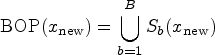
A related concept is the “bag of observations for prediction” (BOP).
9
At a high level, the general modern framework to develop new forest-type methods involves the following steps: (a) design a specialized split rule tailored to the problem at hand; (b) build a forest using this specialized split rule; (c) for a new observation, obtain the NNFWs (or the BOP) and compute the desired parameter using them. Generalized RFs (GRFs)
5
is a method that follows this framework. The same article provides a theoretical justification for using a split criterion that seeks to increase the heterogeneity in the parameter of interest. This approach can be seen as an approximation of a split rule that aims to minimize the least-squares criterion for this parameter (refer to Proposition 1 in that article). In practice, this approach performs well and has been applied in various contexts. For instance, an early example involves using the log-rank test as the split rule with survival data.
10
The log-rank test aims to maximize the heterogeneity of the conditional survival function (an unknown quantity for all subjects). Other examples of this approach in different settings include works by Moradian et al.,
11
Tabib and Larocque,
9
and Alakuş et al.12,13
It is also possible to use
Local centering of the response and/or the treatment variable is now recognized as being an important strategy for improving performance, especially in the presence of confounding, 16 which is one of the main challenges for CATE estimation. However, less attention has been given to collider bias17,18 even though including a collider variable in the model can have a detrimental effect.
Motivated by the above discussion, this article presents an empirical study to investigate RFs for CATE estimation. The study incorporates the following elements and characteristics: (a) it utilizes a continuous treatment, as this situation has been less studied; (b) it includes RFs from both approaches described earlier; (c) it employs data-generating processes (DGPs) that incorporate confounding and colliding effects; (d) it explores different variants for preprocessing the data by locally centering the treatment and response.
The work most closely related to this article is Dandl et al. 16 They also investigate several variants of RFs to estimate CATE, but in the case of a binary treatment. In our study, we focus on a continuous treatment, investigate additional aspects such as collider effects, and consider other variants of RF, including new implementations. This allows for more direct comparisons between the methods. A discussion comparing the findings of Dandl et al. 16 and ours is given in Section 3.2.1.
The article is organized as follows. Section 2 describes the problem and methods. Section 3 presents the results from the simulation study. Section 4 provides an illustration using real data. Finally, a discussion and conclusion are presented in Section 5.
Methods
In this section, we define the problem and notation, and describe the investigated methods.
Notation, data, and CATE definition
Let us consider a sample of


Still, assuming a linear model in
The data-generating processes we use satisfy the usual assumptions of positivity and unconfoundedness. The first one states that for any given covariates, all treatment values are possible, that is,
To estimate the CATE at

Given a training sample
Given this general approach, the main question is how to build the RF? We explore variants of the two approaches presented in the Introduction: Approach 1 and Approach 2. While existing implementations are available, they rely on different tree-building algorithms, which can introduce confounding factors when comparing methods. To ensure a more direct and fair comparison, we have implemented our own variants, all based on the same tree-building algorithm following the classification and regression trees (CART) paradigm proposed by Breiman et al. 19
In our study, we implemented two different methods for building decision trees to estimate the CATE. Here is a description of these methods. At a given node
With Approach 1, we want to build trees that seek to increase the heterogeneity of the CATE estimation. To achieve this, we use the following split rule:

With Approach 2, we use

The two methods described above were implemented using the
For Approach 1, the
Another method included in our study is a forest of MOB trees built using the
Local centering variants
As highlighted in the introduction, locally centering the response and the treatment variables is often crucial for enhancing performance. Let
Summary of the methods and specific details for the RF parameters
Table 1 summarizes the methods considered in the study. For methods, HET, CMB, and MOB, four variants are considered by having
Methods investigated in the simulation study.
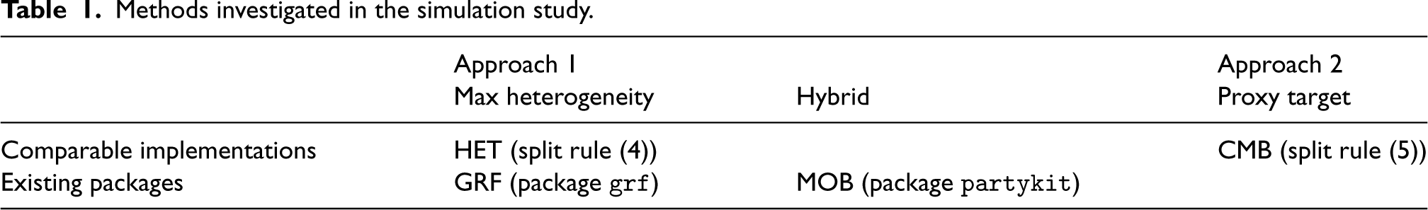
Methods investigated in the simulation study.
For all forests, the number of variables selected at each node (i.e.
In this section, we present the results of a simulation study designed to evaluate the relative performance of the methods to estimate the CATE introduced in the preceding section. We first describe the simulation design and then present the results.
Simulation design
The data-generating processes (DGPs) employed in our study serve the purpose of investigating confounding and colliding effects. Additionally, we incorporate various functional forms for the treatment effect. There are five covariates
The response 
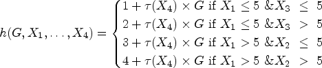
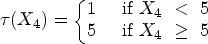
Step treatment effect
Linear treatment effect
Quadratic treatment effect
Two distributions for the treatment variable Randomly uniform. In this case, Correlated with the covariate Independent. In this case, Collider. In this case,
The fifth covariate
In total, we have 27 scenarios (three types of treatment effects (step, linear, and quadratic)
The number of repetitions for each scenario is 100. The training data sample size is 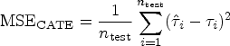
Simulation results
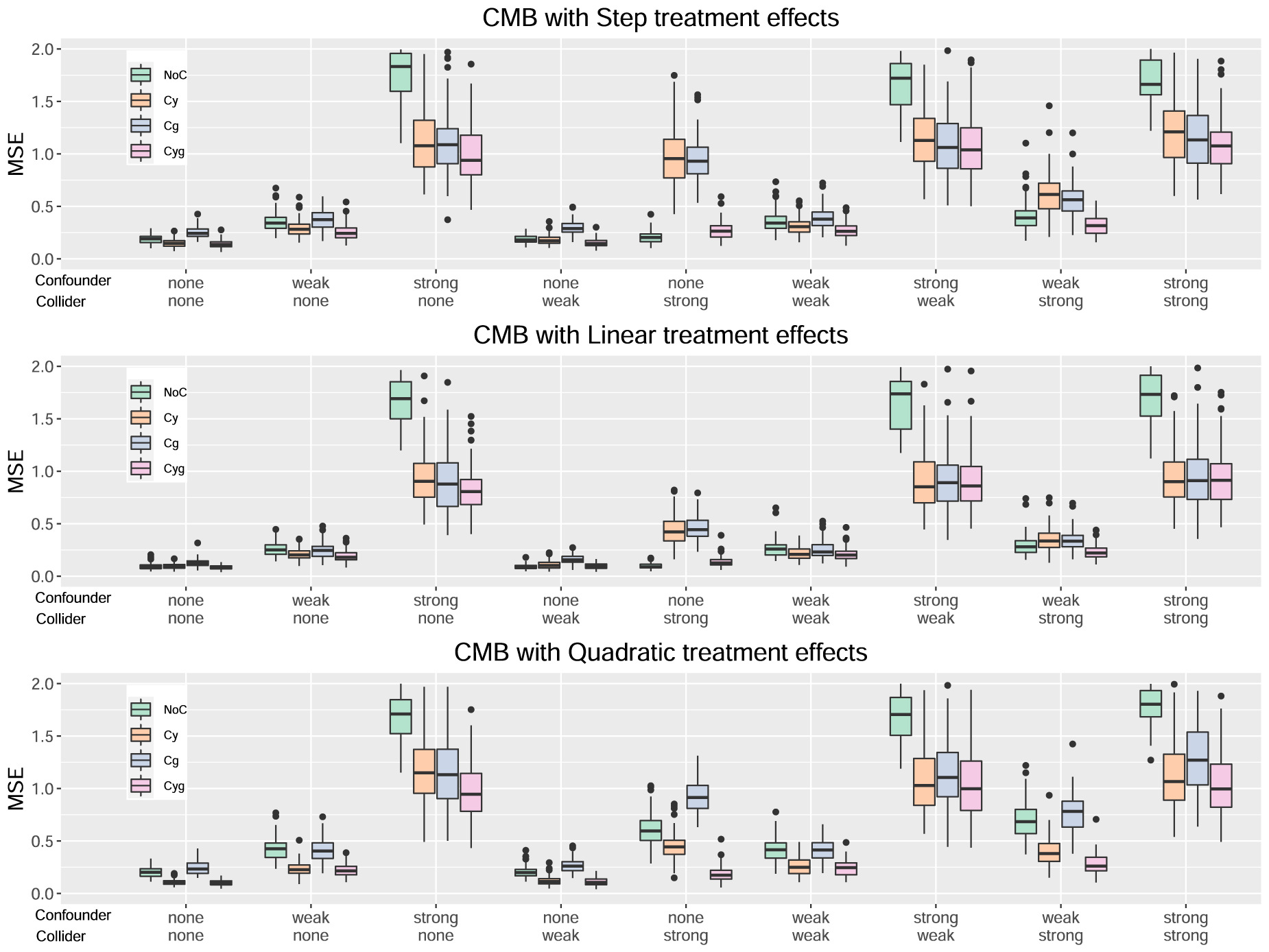
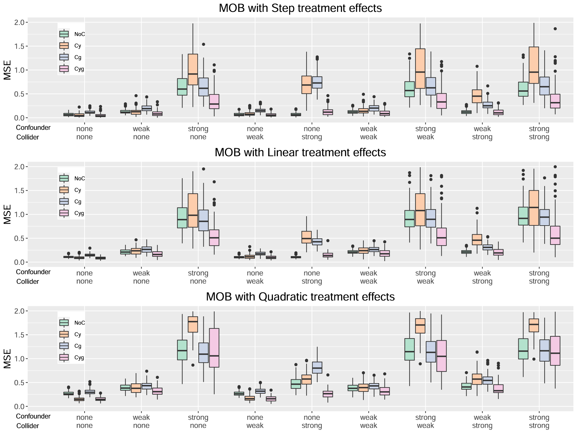
While the main article contains figures that sufficiently convey the primary findings of this study, we also provide additional figures in a separate supplemental material document, including discussions based on the mean absolute error and the C-index as alternative performance measures, as well as comments about the Monte–Carlo error. To ease the discussion, we will denote by NoC, Cy, Cg, and Cyg, the no centering, center Y (response) only, center G (treatment) only, and center both
Locally centering both the response and treatment (Cyg) is generally preferable for all methods considered. When considering the Cyg variants, both approaches, namely splitting based on maximizing the heterogeneity of the treatment effect and splitting to predict the response, are viable. Neither approach dominates the other across all scenarios. In the scenarios considered, the presence of a confounder has a more detrimental impact on performance than that of a collider.
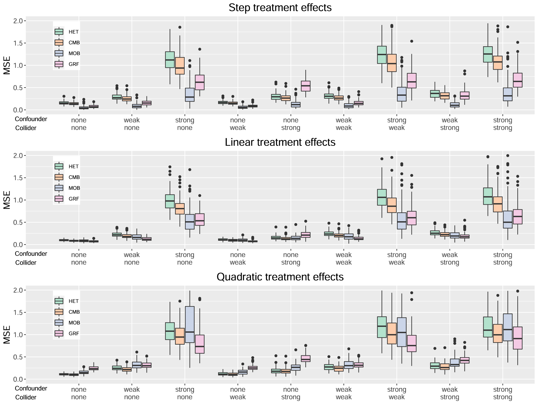
Figures 1 to 4 serve to visualize these general findings and to provide more specific insights. The box plots show the distribution of the mean squared error (MSE) over the 100 simulation runs. Figures 1 to 3 show the performance of all centering variants for a specific method (HET, CMB, and MOB). Recall that only the Cyg variant is considered for GRF since this is the default for this method. Figure 4 compares the four methods HET, CMB, MOB, and GRF, but only their Cyg variant. To aid interpretation, we truncate the
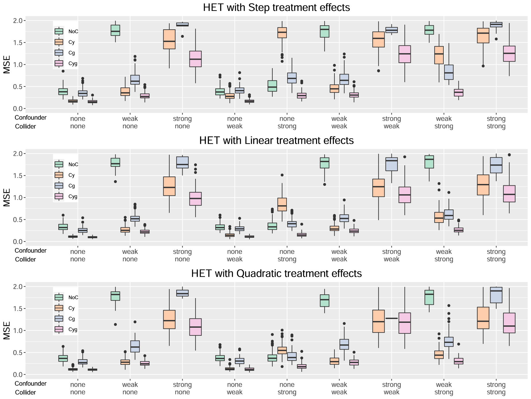
Results for the method HET.
Results for the method CMB.
Results for the method MOB.
Results for all methods, Cyg variant for HET, CMB, and MOB.
For the HET method, from Figure 1, we can observe that the Cyg variant generally performs the best (based on the median mean squared error (MSE)). We can observe that a strong confounder has a more adverse effect on NoC. A strong collider has a more adverse effect on Cy and Cg. Interestingly, the two cases where NoC is slightly better than Cyg are the step and linear treatment effects with a strong collider and no confounder. Another finding, that is also true for the other methods, is that the confounder and collider effects do not interact in a way to multiply their negative effects. Their combined effect is at most additive or even less than that in some cases.
From Figure 2, the patterns observed for the CMB method are very similar to the ones for HET, leading to the same conclusions.
For the MOB method, from Figure 3, the Cyg variant once again emerges as the best choice. We can again observe that a strong collider has a more adverse effect on Cy and Cg. However, unlike the two previous methods, NoC is not the most affected by a strong confounder, as it is Cy this time.
Formal comparisons based on paired-sample
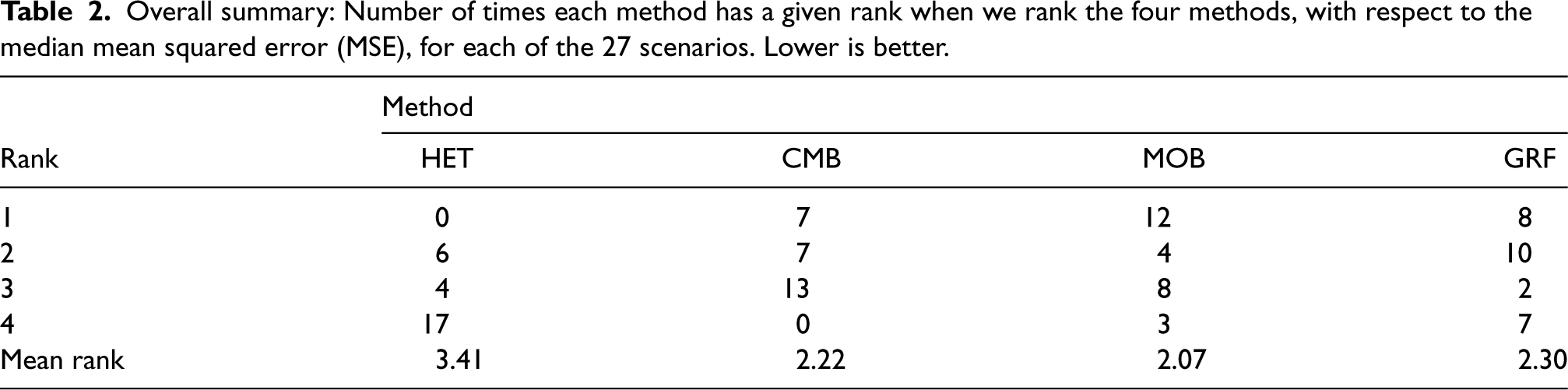
In Figure 4, we directly compare the Cyg variant (the best one) across the four methods. To gain a comprehensive perspective, Table 2 provides the number of times each method has a given rank when we rank the four methods separately for each of the 27 scenarios. A rank of 1 indicates the best performance. Globally, MOB emerges as the top performer in 12 out of 27 scenarios, GRF in eight scenarios, and CMB in seven scenarios. MOB has also the lowest average rank of 2.07, followed by CMB at 2.22 and closely by GRF at 2.3. But keep in mind that the performances are very close in several scenarios as seen in Figure 4. For example, even if HET is not the single best method in any scenario, its performance is very close to the one of CMB in general and, consequently, it often comes in second place in scenarios where CMB is the best method (see Table 3 for more details).
Looking at each type of treatment effect separately, we see that MOB has the best performance for the step treatment effect (upper plot). For the linear treatment effect (middle plot), the best method is either MOB or GRF. For the quadratic treatment effect (lower plot), the best method is either CMB or GRF. We also note that GRF is the worst when there is a strong collider alone. But on the other hand, it is one of the two best methods when there is a strong confounder alone.
Comparing two methods at a time is also interesting. Table 3 presents the results for interesting pairs which are discussed in the following.
The two methods that are the more directly comparable without interference from specific aspects of the tree and forest implementations are HET and CMB. Recall that these two methods share exactly the same tree and forest building architecture, and only the splitting rules they use are different. We can see in Figure 4 that CMB and HET are very close but CMB has a slight advantage in all scenarios and most notably in the ones with a strong confounder. The paired-sample
The direct comparison of MOB and CMB is also of interest. MOB is a hybrid approach between Approaches 1 and 2. CMB is a “pure” Approach 2 method. MOB significantly outperforms CMB in 15 out of 27 scenarios and the difference in mean MSE exceeds 20% for 12 of them. Conversely, CMB significantly outperforms MOB in 10 out of 27 scenarios, and the difference in mean MSE exceeds 20% for 7 of them. MOB is generally better than CMB for the step treatment effects scenarios but the opposite occurs for the quadratic treatment effect. This highlights that even without incorporating directly the heterogeneity maximizing component, a method based on a proxy target can be competitive.
The direct comparison between MOB and GRF is also of interest as they are two existing methods prior to this article. In 14 out of 27 scenarios, MOB significantly outperforms the CMB. Conversely, in eight out of 27 scenarios, CMB significantly outperforms MOB. Further discussions related to Dandl et al. 16 can be found in the next subsection.
The direct comparison between GRF and HET is also of interest as they are two methods from Approach 1. They are based on very similar ideas and rely on the CART paradigm. HET uses directly a split rule that seeks to maximize the heterogeneity in the treatment effect, while GRF uses an approximate version of it. Other specific details in the GRF implementation might explain the differences we find but, in the end, GRF significantly outperforms HET in 19 out of 27 scenarios. Conversely, HET significantly outperforms GRF in eight scenarios.
In their empirical investigation, Dandl et al.
16
explore various variants of RFs for estimating treatment effects in the context of binary treatments. In our study, we extend this analysis by focusing on continuous treatments and examining additional aspects, including collider effects. We also include other variants such as the CART version of MOB. It is possible to compare some of the general conclusions of both articles. The variant Cyg of MOB we use in our study is basically the method called
Real data example
In this section, we present an illustration using data from the 1987 National Medical Expenditure Survey. The goal is to investigate the impact of smoking on medical expenditure. These data have been analyzed in Johnson et al.,
27
Imai and Van Dyk,
28
and Hahn et al.
29
We use the data available in the package
Overall summary: Number of times each method has a given rank when we rank the four methods, with respect to the median mean squared error (MSE), for each of the 27 scenarios. Lower is better.
Overall summary: Number of times each method has a given rank when we rank the four methods, with respect to the median mean squared error (MSE), for each of the 27 scenarios. Lower is better.
Some relevant paired comparisons.
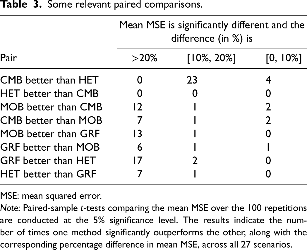
MSE: mean squared error.
Note: Paired-sample
For this example, we use the following covariates and keep the names provided in the package to facilitate the description and references:
AGESMOKE: age when the individual started smoking (in years). LASTAGE: age in years at the time of the survey (in years). MALE: gender (male or female). RACE3: black, white or other. BELTUSE: use a seat belt when in a car regularly (yes or no). EDUCATE education level (college graduate, some college, high school graduate, and other). MARITAL: marital status (married, widowed, divorced, separated, and never married). POVSTALB: poverty status (poor, near poor, low income, middle income, and high income).
The observed response is the annual medical expenditure, but this variable exhibits significant skewness. Consequently, following the approach of Imai and Van Dyk
28
and Hahn et al.,
29
we take its natural logarithm as the outcome. The level of smoking serves as our treatment variable. As proposed in Johnson et al.,
27
we capture the smoking effect using the variable “packyears,” which represents the number of cigarettes per day times the number of years smoked divided by 20. Finally, we made a standardization to the packyears variable to ensure it is in the [0,1] range. Following Johnson et al.
27
and Imai and Van Dyk,
28
we retain only patients with positive medical expenditures and exclude records with missing values. Our final sample consists of
Data analysis
We employ the same four methods used in the simulation study to estimate treatment effects. For HET, CMB, and MOB, the Cyg (center the response and the treatment) variant is used. However, for reasons explained below, we also consider the NoC variant for MOB and the GRF variant with Variable importance for the smoking effect example.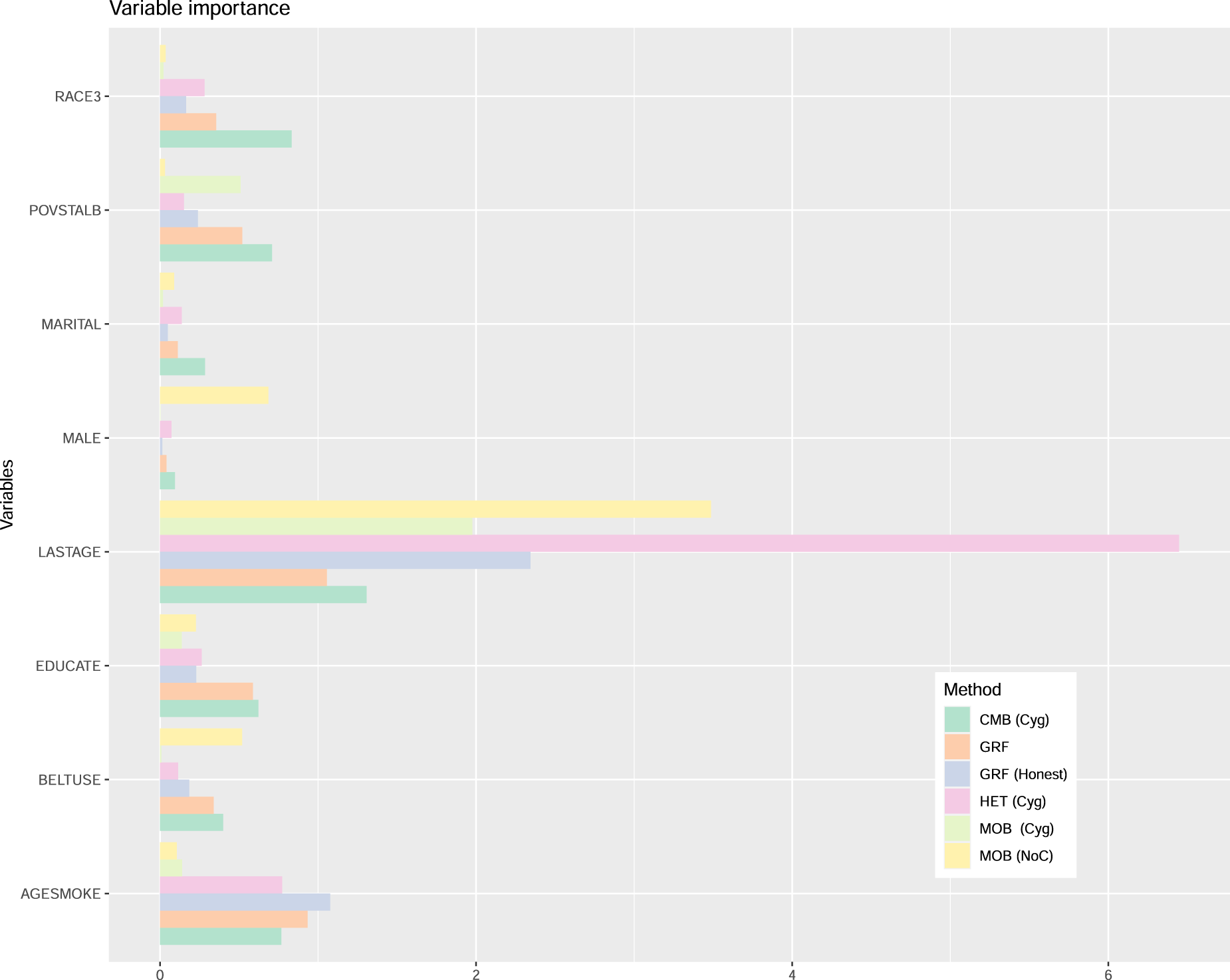
Figure 5 presents the variable importance measures. For all methods, LASTAGE is the most important variable. To explore the effect of this variable, Figure 6 displays the partial dependence plots for all methods, focusing on the age range between 30 and 70 years old. The curve for HET exhibits greater variability at lower age values, which corresponds to a region with less available data, making visual analysis more challenging. The complete curves spanning the entire age range are provided in the supplemental material. The general pattern holds true for HET (Cyg), CMB (Cyg), and GRF: the age effect is more pronounced before 40 years old, after which it decreases and stabilizes. However, the pattern diverges for MOB (Cyg), where we observe a small yet consistent (possibly slightly decreasing) treatment effect across all ages. To explore further, we also present the curve for the NoC variant MOB (NoC). Interestingly, this pattern aligns more closely with that of HET (Cyg), CMB (Cyg), and GRF. The supplemental material presents similar graphs for HET (NoC) and CMB (NoC) where we find that the patterns remain the same as for their Cyg variants. Thus, whether we center both the treatment and the response does not significantly impact HET and CMB with this dataset, but it does play a crucial role for MOB. Additionally, Figure 6 also shows the GRF variant with
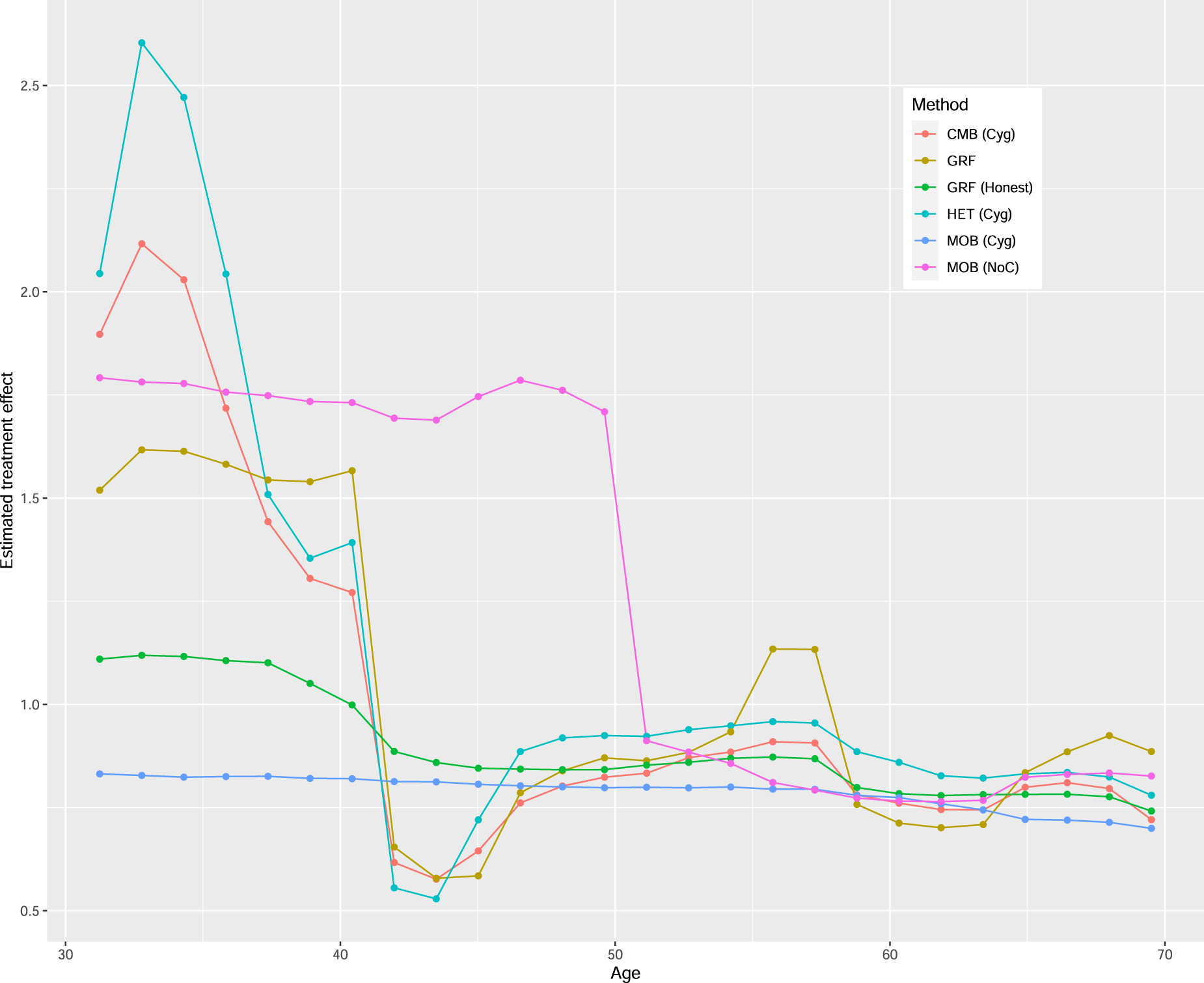
Partial dependence plots of the age (LASTAGE) effect in the example.
These general findings align with those reported in section 7 (see Figure 9 in Hahn et al.
29
), where the data were analyzed using a binary treatment (a binary version of packyears). Notably, the study also highlights that the impact of age on the treatment effect can vary depending on the chosen method. In their analysis, the method specifically designed to detect treatment effects (referred to as BCF) indeed detects a more pronounced heterogeneity moderated by age. They also conclude:
From the above we conclude that how a model treats the age variable would seem to have an outsized impact on the way that predictive patterns are decomposed into treatment effect estimates based on this data, as age plausibly has prognostic, propensity and moderating roles simultaneously.
In our own analysis, both CMB and HET reveal similar treatment effect heterogeneity moderated by age, even if the split rule used by CMB is not specifically designed to increase the heterogeneity of the treatment effect, as opposed to the one used by HET, which is intentionally designed to do so.
These results raise additional methodological and practical questions, which we discuss in the conclusion.
Based on the findings from our simulation study, the most important recommendation is that locally centering both the response and treatment variables should be the default strategy. Second, all approaches considered perform well. That is, building trees with a split rule that seeks to increase the heterogeneity of the CATE and building trees to predict
While we explored various scenarios and methods in our simulation study, there are still other aspects that warrant investigation in future research. The first aspect is about the DGPs. The main focus of our study was to investigate the impact of confounder and collider variables. While we considered different versions for the treatment effect
The results from the real data analysis provide valuable insights for potential future work and practical guidelines. In practice, it is advisable to employ multiple methods and their variants when analyzing the same dataset. This approach serves as a sensitivity analysis. Given that a direct and objective performance measure for estimating treatment effects is unavailable, determining the appropriate course of action when faced with divergent results from different methods would be interesting future work. Additionally, future research could investigate the circumstances under which using the honest version of GRF is preferable.
While the semi-parametric model (2) offers flexibility, it assumes a linear model between 
Supplemental Material
sj-pdf-1-smm-10.1177_09622802241275401 - Supplemental material for Comparison of random forest methods for conditional average treatment effect estimation with a continuous treatment
Supplemental material, sj-pdf-1-smm-10.1177_09622802241275401 for Comparison of random forest methods for conditional average treatment effect estimation with a continuous treatment by Sami Tabib and Denis Larocque in Statistical Methods in Medical Research
Footnotes
Acknowledgements
We would like to warmly thank three reviewers and two associate editors for their insightful, helpful, and constructive comments about this work that paved the way for this version of the article.
Declaration of conflicting interests
The authors declared no potential conflicts of interest with respect to the research, authorship, and/or publication of this article.
Funding
The authors received no financial support for the research, authorship, and/or publication of this article.
Supplemental material
Supplemental material for this article are available online.
References
Supplementary Material
Please find the following supplemental material available below.
For Open Access articles published under a Creative Commons License, all supplemental material carries the same license as the article it is associated with.
For non-Open Access articles published, all supplemental material carries a non-exclusive license, and permission requests for re-use of supplemental material or any part of supplemental material shall be sent directly to the copyright owner as specified in the copyright notice associated with the article.