Multivariate Poisson cokriging: A geostatistical model for health count data

Abstract

Multivariate disease mapping is important for public health research, as it provides insights into spatial patterns of health outcomes. Geostatistical methods that are widely used for mapping spatially correlated health data encounter challenges when dealing with spatial count data. These include heterogeneity, zero-inflated distributions and unreliable estimation, and lead to difficulties when estimating spatial dependence and poor predictions. Variability in population sizes further complicates risk estimation from the counts. This study introduces multivariate Poisson cokriging for predicting and filtering out disease risk. Pairwise correlations between the target variable and multiple ancillary variables are included. By means of a simulation experiment and an application to human immunodeficiency virus incidence and sexually transmitted diseases data in Pennsylvania, we demonstrate accurate disease risk estimation that captures fine-scale variation. This method is compared with ordinary Poisson kriging in prediction and smoothing. Results of the simulation study show a reduction in the mean square prediction error when utilizing auxiliary correlated variables, with mean square prediction error values decreasing by up to 50%. This gain is further evident in the real data analysis, where Poisson cokriging yields a 74% drop in mean square prediction error relative to Poisson kriging, underscoring the value of incorporating secondary information. The findings of this work stress on the potential of Poisson cokriging in disease mapping and surveillance, offering richer risk predictions, better representation of spatial interdependencies, and identification of high-risk and low-risk areas.

1. Introduction

Multivariate disease mapping plays a vital role in public health research by providing valuable insights into the spatial distribution and patterns of health outcomes and putative risk factors. It aims to identify shared risk factors, establish relationships between diseases and implement integrated disease surveillance systems. Geostatistical methods are valuable for analyzing spatially dependent health data, enabling the modeling and predicting of disease rates across geographical regions. ¹ Nonetheless, when dealing with spatial counts, such as the number of disease cases, several challenges arise within the geostatistics framework.

Traditional geostatistical methods, such as kriging, struggle to accurately model disease count data due to the heterogeneous nature of the observed cases and the frequent presence of low count distributions. It often yields improper estimation of the spatial dependence, over smoothed risk predictions and poor prediction uncertainty.^2–5 Disease risk estimation procedures, which require the division of observed cases between the population sizes, further aggravate these issues. The resulting raw risk distributions are heavy-tailed, highly asymmetric and unreliable given the inherent spatial variability of population sizes.

To face these challenges, the geostatistical literature offers a range of methods for modeling disease count data. Binomial cokriging ⁶ and beta-binomial kriging ⁷ were developed to handle disease proportions derived from disease counts. Such proportions typically result in loss of information and biased inference. ⁸ In disease mapping analyses, counts are generally preferred due to their ability to handle small counts and facilitate detailed spatial analysis. Poisson kriging, introduced by Monestiez et al. ² and extended and applied to disease count data,^3,4,9–11 has stood as a prominent geostatistical method for analyzing disease count data. Poisson kriging allows inferring the underlying disease risk while accounting for the non-stationarity of the observed disease counts induced by the population size variability. Payares-Garcia et al. ⁵ extended this methodology to operate in a bivariate context, addressing challenges posed by sparse observations and allowing for the estimation of disease risk at locations with absent or inaccessible data but with information available on a closely related disease. The model enhanced risk prediction precision, captured diseases’ geographical cross-correlation and produced smoothed risk maps accurately mirroring the underlying disease risk. Restricting the analysis to bivariate disease interactions, however, fails to fully exploit the potential of cokriging and to meet the increasing need for multivariate disease mapping.

Outside the multivariate geostatistics domain, Bayesian hierarchical models are useful for multivariate mapping of disease counts. Their widespread adoption remains, however, constrained due to limited user-friendly software implementations and substantial computational costs of Markov chain Monte Carlo and integrated nested Laplace approximation estimation, particularly when the number of diseases increases.^12,13 The primary modeling strategies of shared component models ¹⁴ and multivariate spatial distributions, such as the multivariate conditional autoregressive,^15–17 coregionalization,^18,19 model-based geostatistics, ¹ and computationally efficient M-models frameworks, ²⁰ are hard to scale to large spatial datasets, with inference becoming prohibitive at times. The selection of an appropriate prior distribution poses as well practical challenges to non-experts in the domain.^4,9 While valuable, multivariate disease mapping outside of geostatistics often grapples with computational, interpretability and scalability obstacles. Cokriging integrates multivariate dependence and ancillary information using accessible, interpretable, and rapid estimation procedures. Likewise the ability of cokriging to predict at unobserved locations, makes it an advantageous tool against its counterparts for multivariate mapping.

In this study, we present a generalization of Poisson cokriging for the prediction and smoothing of multivariate disease spatial counts. It capitalizes on the pair-wise correlation between a target variable and multiple ancillary variables in the form of disease counts. Building upon the model proposed by Payares-Garcia et al., ⁵ we adopt a pair-wise covariance model, as a specific instance of the multivariate Poisson distribution as outlined by Mahamunulu. ²¹ The proposed methodology for multivariate disease mapping has critical implications for public health planning and interventions. By enabling precise identification of geographical disease clusters and at-risk populations, this method supports policymakers in strategic resource allocation and targeted prevention programming.

The article is organized as follows. First, we provide a detailed exposition of the mathematical foundations of Poisson cokriging and elucidate the theoretical principles that underpin its development. Then, we illustrate our model’s prediction and smoothing capabilities by means of a comprehensive simulation analysis and a real data application to human immunodeficiency virus (HIV) incidence and sexually transmited diseases (STDs) data in Pennsylvania. The results and implications of our research are synthesized and discussed in the final section, providing a comprehensive summary of our findings.

2. Statistical modeling

2.1. Model

Let ( ${\mathcal{R}}_1(\mathbf{s}),\dots ,{\mathcal{R}}_{\mathcal{L}}(\mathbf{s})$ ) be a multivariate spatial vector of $\mathcal{L}$ dependent positive random fields on a region $\mathcal{D}\subset {\mathbb{R}}^2$ . These $\mathcal{L}$ fields are assumed to represent unobserved spatially varying disease risks at any given location $\mathbf{s}\in \mathcal{D}$ . To learn about these unobserved risks, spatial data are collected on the spatial vector of $\mathcal{L}$ random Poisson variables ( $Y_{1i},\dots ,Y_{\mathcal{L}i}$ ) representing the number of disease cases for each of the $\mathcal{L}$ diseases at sampling locations ${\mathbf{s}}_i$ , $i=1,2,\dots ,k$ .

The vector of disease counts ( $Y_{1i},\dots ,Y_{\mathcal{L}i}$ ) is assumed to follow a Poisson multivariate joint distribution with $\mathcal{L}+{\displaystyle (\genfrac{}{}{0ex}{}{\mathcal{L}}{2})}$ nonnegative parameters ${\theta }_{1i},\dots ,{\theta }_{\mathcal{L}i},{\theta }_{12i},\dots ,{\theta }_{1\mathcal{L}i}$ $,\dots ,{\theta }_{\mathcal{L}-1,\mathcal{L},i}$ where the subscripts on a particular $\theta$ represent those of the $Y$ ’s in which the corresponding Poisson variable appears as a summand and the sampling location ${\mathbf{s}}_i$ . Let the $\ell$ -th random variable $Y_{\ell i}$ be written as,

$$Y_{\ell i}=X_{\ell i}+X_{\ell 1i}+\cdots +X_{\ell \mathcal{L}i}$$

(1)

where every $X_{\ell \kappa i}$ is an independent Poisson distributed random variable with parameter ${\theta }_{\ell \kappa i}$ , with $\ell ,\kappa =1,2,\dots ,\mathcal{L}$ and $i=1,2,\dots ,k$ .

In disease mapping, the parameter ${\theta }_{\ell \kappa i}=n_{\ell \kappa i}\cdot r_{\ell \kappa }({\mathbf{s}}_i)$ denotes the incidence as the product between the population size $n_{\ell \kappa i}$ and the marginal ( $\ell =\kappa$ ) or joint ( $\ell \ne \kappa$ ) disease risk $r_{\ell \kappa }({\mathbf{s}}_i)$ . We take the population size $n_{\ell \kappa i}$ identical for every combination of the $\ell$ -th disease as for each the same population can be infected. Then the counts $Y_{1i},\dots ,Y_{\mathcal{L}i}$ are conditionally independent given the risks $r_{\ell \kappa }({\mathbf{s}}_i)$ for a set of sampling locations $s_i\in \mathcal{D}$ , ⁴ and the following model is obtained for all $\ell =1,2,\dots ,\mathcal{L}$

$$Y_{\ell i}\mid {\mathcal{R}}_{\ell }({\mathbf{s}}_i)\sim \text{Poisson}(n_{\ell i}\cdot {\mathcal{R}}_{\ell }({\mathbf{s}}_i))$$

(2)

Here, the Poisson parameter of each $Y_{\ell i}$ is the product between the total risk ${\mathcal{R}}_{\ell }({\mathbf{s}}_i)$ and the population size $n_{\ell i}$ at sampling site ${\mathbf{s}}_i$ . The total risk is the term that encompasses the within and between diseases risks, that is, marginal and joint disease risks, $r_{\ell \kappa }({\mathbf{s}}_i)$ such that ${\mathcal{R}}_{\ell }({\mathbf{s}}_i)=\sum _{\kappa =1}^{\mathcal{L}}{r}_{\ell \kappa }({\mathbf{s}}_i)$ . For instance, the total risk ${\mathcal{R}}_{\ell }({\mathbf{s}}_i)$ for the $\ell$ -th disease, equals the sum of the marginal and joint risks of $\ell$ , that is, ${\mathcal{R}}_{\ell }({\mathbf{s}}_i)=r_{\ell }({\mathbf{s}}_i)+r_{1\ell }({\mathbf{s}}_i)+\cdots +r_{\ell \mathcal{L}}({\mathbf{s}}_i)$ . Here, we consider $r_{\ell \ell }(s_i)$ as $r_{\ell }(s_i)$ . The population size $n_{\ell i}$ is assumed to be the same across the $\mathcal{L}$ diseases, implying the model considers a common at-risk population for all processes. The model in (2) assumes different covariances between all pairs in a similar fashion to the multivariate normal distribution. ²²

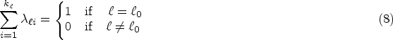
The total set of risk variables ${\mathcal{R}}_{\ell }({\mathbf{s}}_i)$ can be further modeled as positive stationary random fields with means $\sum _{\kappa =1}^{\mathcal{L}}{m}_{\ell \kappa }$ , variances $\sum _{\kappa =1}^{\mathcal{L}}{\sigma }_{\ell \kappa }^2$ , covariance functions $C_{\ell }(|{\mathbf{s}}_i-{\mathbf{s}}_j|)$ and cross-covariance functions $C_{\ell \kappa }(|{\mathbf{s}}_i-{\mathbf{s}}_j|)$ , for $\ell ,\kappa =1,2,3,\dots ,\mathcal{L}$ . The notation $|\cdot |$ indicates the Euclidean distance between locations. Note that the mean and variance of the ${\mathcal{R}}_{\ell }({\mathbf{s}}_i)$ are the sum of marginal means and variances of the marginal and joint risks. This characteristic is attributed to the independence between the Poisson parameters. Likewise, we assume that the covariance and cross-covariance functions solely rely on the absolute values of the distances between the sites ${\mathbf{s}}_i$ and ${\mathbf{s}}_j$ , and not on their direction.

Following Monestiez et al., ² Goovaerts, ⁴ and Payares-Garcia et al., ⁵ the conditional mean and variance of variable $Y_{\ell }({\mathbf{s}}_i)$ from the set of $\mathcal{L}$ variables are defined as follows:

$$\begin{array}{rl}\mathrm{E}[Y_{\ell i}\mid {\mathcal{R}}_{\ell }({\mathbf{s}}_i)]& =n_{\ell i}{\mathcal{R}}_{\ell }({\mathbf{s}}_i)\\ \mathrm{Var}[Y_{\ell i}\mid {\mathcal{R}}_{\ell }({\mathbf{s}}_i)]& =n_{\ell i}{\mathcal{R}}_{\ell }({\mathbf{s}}_i)\end{array}$$

and the unconditional mean and variance:

$$\begin{array}{rl}\mathrm{E}[Y_{\ell i}]& =n_{\ell i}\sum _{\kappa =1}^{\mathcal{L}}{m}_{\ell \kappa }\\ \mathrm{Var}[Y_{\ell i}]& =n_{\ell i}\sum _{\kappa =1}^{\mathcal{L}}{m}_{\ell \kappa }+n_{\ell i}^2\sum _{\kappa =1}^{\mathcal{L}}{\sigma }_{\ell \kappa }^2\end{array}$$

(3)

The intra and inter-dependency among the random variables at different sites is predicated upon the pair-wise variance and covariance between the $\mathcal{L}$ diseases given the conditional independence of observations. We then obtain between two sites $i$ and $j$

$$\begin{array}{rl}\mathrm{E}[Y_{\ell i}{Y}_{\ell j}\mid {\mathcal{R}}_{\ell }]& =\mathrm{Cov}[Y_{\ell i},Y_{\ell j}\mid {\mathcal{R}}_{\ell }]+\mathrm{E}[Y_{\ell i}\mid {\mathcal{R}}_{\ell }({\mathbf{s}}_i)]\mathrm{E}[Y_{\ell j}\mid {\mathcal{R}}_{\ell }({\mathbf{s}}_j)]\\ & ={\delta }_{ij}{n}_{\ell i}{\mathcal{R}}_{\ell }({\mathbf{s}}_i)+n_{\ell i}{\mathcal{R}}_{\ell }({\mathbf{s}}_i)\cdot n_{\ell j}{\mathcal{R}}_{\ell }({\mathbf{s}}_j)\end{array}$$

(4)

and between two diseases $\ell$ and $\kappa$

$$\begin{array}{rl}\mathrm{E}[Y_{\ell i}{Y}_{\kappa j}\mid \mathcal{R}]& =\mathrm{Cov}[Y_{\ell i},Y_{\kappa j}\mid \mathcal{R}]+\mathrm{E}[Y_{\ell i}\mid {\mathcal{R}}_{\ell }({\mathbf{s}}_i)]\mathrm{E}[Y_{\kappa j}\mid {\mathcal{R}}_{\kappa }({\mathbf{s}}_j)]\\ & ={\delta }_{ij}{n}_{\ell i}{r}_{\ell \kappa }({\mathbf{s}}_i)+n_{\ell i}{\mathcal{R}}_{\ell }({\mathbf{s}}_i)\cdot n_{\kappa j}{\mathcal{R}}_{\kappa }({\mathbf{s}}_j)\end{array}$$

(5)

where ${\delta }_{ij}$ is the Kronecker delta. ${\delta }_{ij}=\{\begin{array}{lll}0& \text{if}& i\ne j\\ 1& \text{if}& i=j\end{array}$ indicating the conditional independence between locations.

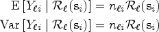
The covariance terms in (4) and (5) can be expressed in matrix form as follows:

$$\begin{array}{rl}\mathrm{Var}[\mathbf{Y}\mid \mathcal{R}]& ={\delta }_{ij}\left[\begin{array}{ccc}{n}_{1i}& & \\ & \ddots & \\ & & n_{\mathcal{L}i}\end{array}\right]\left[\begin{array}{ccc}{\mathcal{R}}_1({\mathbf{s}}_i)& \cdots & r_{1\mathcal{L}}({\mathbf{s}}_i)\\ ⋮& \ddots & ⋮\\ r_{\mathcal{L}1}({\mathbf{s}}_i)& \cdots & {\mathcal{R}}_{\mathcal{L}}({\mathbf{s}}_i)\end{array}\right]\\ & ={\delta }_{ij}\left[\begin{array}{ccc}{n}_{1i}& & \\ & \ddots & \\ & & n_{\mathcal{L}i}\end{array}\right]\left[\begin{array}{ccc}\sum _{\kappa =1}^{\mathcal{L}}{r}_{1\kappa }({\mathbf{s}}_i)& \cdots & r_{1\mathcal{L}}({\mathbf{s}}_i)\\ ⋮& \ddots & ⋮\\ r_{\mathcal{L}1}({\mathbf{s}}_i)& \cdots & \sum _{\kappa =1}^{\mathcal{L}}{r}_{\mathcal{L}\kappa }({\mathbf{s}}_i)\end{array}\right]\end{array}$$

(6)

The variance within disease $\ell$ is equivalent to the product of the population size $n_{\ell i}$ and the total risk ${\mathcal{R}}_{\ell }({\mathbf{s}}_i)$ which sums up the combined effects of both the marginal risk and the joint risk associated with that specific disease at location ${\mathbf{s}}_i$ , that is, $\sum _{\kappa =1}^{\mathcal{L}}{r}_{\ell \kappa }({\mathbf{s}}_i)$ for $\kappa =1,2,\dots ,\mathcal{L}$ . The covariance between diseases $\ell$ and $\kappa$ represents the product between the population size and the joint risk shared between these two diseases $r_{\ell \kappa }({\mathbf{s}}_i)$ , indicating their pair-wise covariance.

2.2. Poisson cokriging

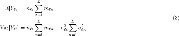
Kriging of the total risk ${\mathcal{R}}_{{\ell }_0}({\mathbf{s}}_0)$ at any site $s_0\in \mathcal{D}$ for disease ${\ell }_0\in \mathcal{L}$ is a linear combination of weights ${\lambda }_{\ell i}$ with data from the observed disease counts $Y_{\ell i}$ divided by their corresponding population sizes $n_{\ell i}$ . Possibly different sample sizes are denoted by $k_{\ell }$ for the $\mathcal{L}$ diseases. Kriging is then expressed as follows:

$${\mathcal{R}}_{{\ell }_0}^{*}({\mathbf{s}}_0)=\sum _{\ell =1}^{\mathcal{L}}\sum _{i=1}^{k_{\ell }}{\lambda }_{\ell i}\frac{Y_{\ell i}}{n_{\ell i}}$$

(7)

The unbiasedness constraint imposes a set of weights on the variables, ensuring that they sum up to one for the variable of interest ${\ell }_0$ , while having a zero sum for the auxiliary variables

$$\sum _{i=1}^{k_{\ell }}{\lambda }_{\ell i}=\{\begin{array}{ccc}1& \text{if}& \ell ={\ell }_0\\ 0& \text{if}& \ell \ne {\ell }_0\end{array}$$

(8)

The weights in (8) are the solution to the Poisson cokriging system of linear equations

$$\{\begin{array}{l}\frac{{\lambda }_{\ell i}}{n_{\ell i}}\sum _{\kappa =1}^{\mathcal{L}}{m}_{\ell \kappa }+\frac{{\lambda }_{\kappa i}}{n_{\ell i}}{m}_{\ell \kappa }+\sum _{\kappa =1}^{\mathcal{L}}\sum _{j=1}^{k_{\ell }}{\lambda }_{\kappa j}{C}_{\ell \kappa ij}^{\mathcal{R}}+{\mu }_{\ell }=C_{\ell {\ell }_{0}0i}^{\mathcal{R}}\text{ for }\ell =1,2,\dots ,\mathcal{L};i=1,\dots ,k_{\ell }\\ \sum _{i=1}^{k_{\ell }}{\lambda }_{{\ell }_{0}i}=1\\ \sum _{\begin{array}{c}\ell =1\\ \ell \ne {\ell }_0\end{array}}^{\mathcal{L}}\sum _{i=1}^{k_{\ell }}{\lambda }_{\ell i}=0\end{array}$$

(9)

The symbol ${\mu }_{\ell }$ denotes the Lagrange parameter associated with the $\ell$ -th variable, which is used during the minimization process. In (9), the terms $C_{\ell \kappa ij}^{\mathcal{R}}\text{ and }{C}_{\ell {\ell }_{0}i0}^{\mathcal{R}}$ are equal to $C_{\ell \kappa }^{\mathcal{R}}(|{\mathbf{s}}_i-{\mathbf{s}}_j|)\text{ and }{C}_{\ell {\ell }_0}^{\mathcal{R}}(|{\mathbf{s}}_i-{\mathbf{s}}_0|)$ , respectively. The system presented in equation (9) is formulated in terms of covariances rather than semivariograms, but it can be readily transformed by utilizing the relationship between the covariance and the semivariogram, ²³ ${\gamma }_{\ell \kappa ij}^{\mathcal{R}}=C_{\ell \kappa ii}^{\mathcal{R}}-\frac{1}{2}(C_{\ell \kappa ij}^{\mathcal{R}}+C_{\ell \kappa ji}^{\mathcal{R}})$ . The matrix representation of the Poisson cokriging system of equations is detailed in Appendix A.1.

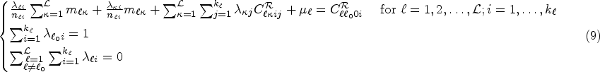
Note that the terms $\frac{1}{n_{\ell i}}\sum _{\kappa =1}^{\mathcal{L}}{m}_{\ell \kappa }$ and $\frac{1}{n_{\ell i}}{m}_{\ell \kappa }$ correspond to the bias term accounting for the variability induced by the inversely proportional relationship between the population sizes and the risk variance, that is, $\mathrm{Var}[{\mathcal{R}}_{\ell }({\mathbf{s}}_i)]\propto n_{\ell i}$ , if locations ${\mathbf{s}}_i$ and ${\mathbf{s}}_j$ coincide for the diseases $\ell$ and $\kappa$ . As in (6), the bias terms depend upon the pair-wise variance and covariance between $\ell$ and $\kappa$ , that is,

$$\begin{array}{rl}& \{\begin{array}{lll}\frac{1}{n_{\ell i}}\sum _{\kappa =1}^{\mathcal{L}}{m}_{\ell \kappa }& \text{if}& \ell =\kappa \\ \frac{1}{n_{\ell i}}{m}_{\ell \kappa }& \text{if}& \ell \ne \kappa \end{array}\end{array}$$

(10)

Finally, the prediction error variance pertaining to the Poisson cokriging estimator presented in equation (7) can be expressed as follows:

$${\sigma }_{\text{{PCK}}}^2({\mathbf{s}}_0)=\sum _{\kappa =1}^{\mathcal{L}}{\sigma }_{{\ell }_0\kappa }^2-\sum _{\ell =1}^{\mathcal{L}}\sum _{i=1}^{k_{\ell }}{\lambda }_{\ell i}{C}_{{\ell }_0\ell 0i}-{\mu }_{{\ell }_0}$$

(11)

The covariance functions $C_{\ell \kappa ij}^{\mathcal{R}}$ required to obtain the kriging weights and kriging variance, as depicted in (9) and (11), are estimated using semivariogram estimators in order to characterize the dependence within the spatial process ${\mathcal{R}}_{\ell }(\mathbf{s})$ . Details on (9) and (11) can be found in Appendix A.2.

2.3. Semivariogram and cross-semivariograms

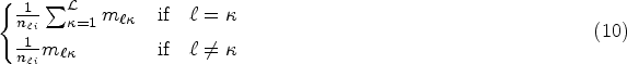
In our analysis, we adopt a generalized formulation of the empirical semivariogram estimators ${\gamma }_{\alpha }^{\mathcal{R}}(\mathbf{h})$ and ${\gamma }_{\alpha \beta }^{\mathcal{R}}(\mathbf{h})$ proposed by Payares-Garcia et al. ⁵ to examine the diseases’ risk under the presence of spatially varying populations.

Let $Y_{\ell i}$ and $Y_{\kappa j}$ be the sample counts and $n_{\ell i}$ and $n_{\kappa j}$ the observed population sizes for any ${\mathbf{s}}_i,{\mathbf{s}}_j\in \mathcal{D}$ and all pairs of diseases $\ell ,\kappa =1,2,\dots ,\mathcal{L}$ . Estimating the semivariogram for the risk of the $\ell$ -th disease can be expressed as follows:

$${\gamma }_{\ell }^{\mathcal{R}}(\mathbf{h})=\frac{1}{2\sum _{(i,j)\in N(\mathbf{h})}{w}_{ij}}\sum _{i,j}(w_{ij}{(\frac{Y_{\ell i}}{n_{\ell i}}-\frac{Y_{\ell j}}{n_{\ell j}})}^2-\sum _{\kappa =1}^{\mathcal{L}}{m}_{\ell \kappa }^{*})$$

(12)

where $N(\mathbf{h})$ denotes the count of observation pairs separated by a distance $\mathbf{h}$ between locations ${\mathbf{s}}_i$ and ${\mathbf{s}}_j$ , $w_{ij}=\frac{n_{\ell i}{n}_{\ell j}}{n_{\ell i}+n_{\ell j}}$ represents the weighting factor, and $m_{\ell \kappa }^{*}=\frac{\sum n_{\ell i}{r}_{\ell \kappa }(\mathbf{s}i)}{\sum n\ell i}$ corresponds to the estimated mean of the marginal and joint risks.

Similarly, the cross-semivariogram is defined as

$${\gamma }_{\ell \kappa }^{\mathcal{R}}(\mathbf{h})=\frac{1}{2\sum _{(i,j)\in N(\mathbf{h})}{w}_{\ell \kappa }}\sum _{i,j}(w_{\ell \kappa }(\frac{Y_{\ell i}}{n_{\ell i}}-\frac{Y_{\ell j}}{n_{\ell j}})(\frac{Y_{\kappa i}}{n_{\kappa i}}-\frac{Y_{\kappa j}}{n_{\kappa j}})-m_{\ell \kappa }^{*})$$

(13)

where $w_{\ell \kappa }=\frac{n_{\ell i}{n}_{\kappa j}}{n_{\ell i}+n_{\kappa j}}$ is the number of observation pairs separated by a distance $\mathbf{h}$ between $i$ and $j$ and $m_{\ell \kappa }^{*}=\frac{\sum n_{\ell i}{r}_{\ell \kappa }({\mathbf{s}}_i)}{\sum n_{\ell i}}$ is the mean estimate of the joint risk $r_{\ell \kappa }({\mathbf{s}}_i)$ . In the case where $\mathcal{L}=2$ , the estimators in (12) and (13) coincide with the semivariogram expressions defined by Payares-Garcia et al. ⁵

In (12) and (13), the inclusion of weights $w_{ij}$ and $w_{\ell \kappa }$ serves to homogenize the variance of the sample rates. Simultaneously, the incorporation of bias terms $\frac{1}{w_{ij}}\sum _{\kappa =1}^{\mathcal{L}}{m}_{\ell \kappa }^{*}$ and $\frac{1}{w_{\ell \kappa }}{m}_{\ell \kappa }^{*}$ mitigates the impact of population-induced variability, particularly in cases where the sample rates are obtained from small population sizes. ²

2.4. Prediction and smoothing of the risk ${\mathcal{R}}_{{\ell }_0}({\mathbf{s}}_{\mathbf{0}})$ for unobserved and observed locations

Let ${\mathcal{R}}_{{\ell }_0}^{*}({\mathbf{s}}_0)$ denote the estimated total risk at target location ${\mathbf{s}}_0\in \mathcal{D}$ for disease ${\ell }_0\in \mathcal{L}$ . In scenarios, where the associated sample risk $\frac{Y_{{\ell }_0}}{n_{{\ell }_0}}$ is unobserved at site ${\mathbf{s}}_0$ for disease ${\ell }_0$ , equation (7) serves as a predictor. Consequently, every available sample rate $\frac{Y_{\ell i}}{n_{\ell i}}$ for $i=1,2,\dots ,k_{\ell }$ and $\ell =1,2,\dots ,\mathcal{L}$ is used to perform the prediction.

In contrast, smoothing is achieved when the sample risk $\frac{Y_{{\ell }_0}}{n_{{\ell }_0}}$ is observed, that is, ${\mathbf{s}}_0$ is any of the sampled ${\mathbf{s}}_i$ . In this case, the sample rate $\frac{Y_{{\ell }_0}}{n_{{\ell }_0}}$ is iteratively removed from the dataset, and the risk ${\mathcal{R}}_{{\ell }_0}({\mathbf{s}}_{[0]})$ at that location is estimated using the remaining $k_{\ell }-1$ samples. The square brackets around the index $0$ symbolize that the estimation is performed at location ${\mathbf{s}}_0$ , excluding its associated sampled risk $\frac{Y_{{\ell }_0}}{n_{{\ell }_0}}$ . This procedure is similar to the traditional geostatistics leave-one-out cross-validation technique. ²³

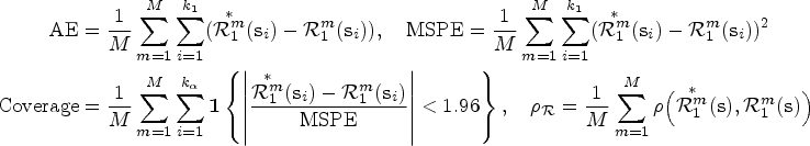
The performance for both the prediction and smoothing processes can be assessed using the average error (AE), the mean squared prediction error (MSPE), and the Pearson’s correlation ( ${\rho }_{\mathcal{R}}$ ) between the estimated values ${\mathcal{R}}_{{\ell }_0}^{*}({\mathbf{s}}_0)$ and the observed values

$$\begin{array}{rl}\mathrm{AE}=& \frac{1}{k_{{\ell }_0}}\sum _{i=1}^{k_{{\ell }_0}}({\mathcal{R}}_{{\ell }_0}^{*}({\mathbf{s}}_i)-{\mathcal{R}}_{{\ell }_0}({\mathbf{s}}_i))\\ \mathrm{MSPE}=& \frac{1}{k_{{\ell }_0}}\sum _{i=1}^{k_{{\ell }_0}}{({\mathcal{R}}_{{\ell }_0}^{*}({\mathbf{s}}_i)-{\mathcal{R}}_{{\ell }_0}({\mathbf{s}}_i))}^2\\ {\rho }_{\mathcal{R}}=& \rho ({\mathcal{R}}_{{\ell }_0}^{*}({\mathbf{s}}_i),{\mathcal{R}}_{{\ell }_0}({\mathbf{s}}_i))\end{array}$$

where $k_{{\ell }_0}$ is the number of locations, ${\mathcal{R}}_{{\ell }_0}^{*}({\mathbf{s}}_i)$ and ${\mathcal{R}}_{{\ell }_0}({\mathbf{s}}_i)$ are the predicted/smoothed and observed risks at location ${\mathbf{s}}_i$ , respectively. The term $\rho$ equals to the Pearson’s correlation function.

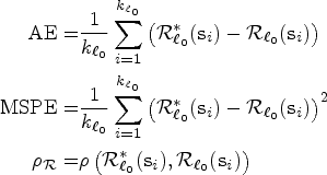
Note that the assessment of the predicted and smoothed risk values is carried out jointly, as predicted values inherently lack ground truth data for independent validation. The AE, MSPE, and ${\rho }_{\mathcal{R}}$ provide a comprehensive evaluation of the Poisson cokriging model’s performance.

3. Simulation studies

3.1. Simulation design

We conducted a simulation study involving 1000 datasets and three distinct diseases ( $\mathcal{L}=3$ ) at 625 sampling locations distributed over a $25\times 25$ grid with coordinates $\mathcal{D}=[-10,10]\times [-10,10]$ with 1.25 units distance between observations. We adopted the model in (2) to generate three log-Gaussian random fields with zero mean ${\mathcal{R}}_1(\mathbf{s})$ , ${\mathcal{R}}_2(\mathbf{s})$ and ${\mathcal{R}}_3(\mathbf{s})$ and the linear model of coregionalization (LMC) to define the underlying spatial structure between the Gaussian latent random fields. The covariance matrix for the LMC is the linear combination of an isotropic exponential covariance function with a range and sill equal to 1 and zero nugget effect, and a spherical structure with a range 5, sill 1 and zero nugget.

The dependence between the sample counts was modeled using Poisson correlation, as discussed by Kawamura. ²⁴ Specifically, we set the Poisson correlations to ${\rho }_{12}^Y=0.25$ , ${\rho }_{13}^Y=0.50$ , and ${\rho }_{23}^Y=0.75$ for the pairs of risks ${\mathcal{R}}_1(\mathbf{s})$ and ${\mathcal{R}}_2(\mathbf{s})$ , ${\mathcal{R}}_1(\mathbf{s})$ and ${\mathcal{R}}_3(\mathbf{s})$ , and ${\mathcal{R}}_2(\mathbf{s})$ and ${\mathcal{R}}_3(\mathbf{s})$ , respectively. Subsequently, three dependent Poisson-distributed sample counts $Y_{1i}$ , $Y_{2i}$ , and $Y_{3i}$ were generated. The population sizes $n_{1i}$ , $n_{2i}$ , and $n_{3i}$ were drawn from a Poisson distribution.

To create a realistic scenario where the target variable ${\mathcal{R}}_1(\mathbf{s})$ is sparsely sampled, but related secondary information ${\mathcal{R}}_2(\mathbf{s})$ and ${\mathcal{R}}_3(\mathbf{s})$ is abundant across the study region, the total risks were partitioned such that the sampling locations of ${\mathcal{R}}_1(\mathbf{s})$ , ${\mathcal{R}}_2(\mathbf{s})$ , and ${\mathcal{R}}_3(\mathbf{s})$ covered 35 $\mathrm{\%}$ , 70 $\mathrm{\%}$ , and 100 $\mathrm{\%}$ of the study area, respectively (Figure 1). The shared locations between the three processes ${\mathcal{R}}_{\alpha }$ and ${\mathcal{R}}_{\beta }$ were used to infer the cross-semivariograms.

Figure 1.

Training sampling locations for the total risk of the diseases $\log {\mathcal{R}}_1({\mathbf{s}}_i)$ , $\log {\mathcal{R}}_2({\mathbf{s}}_i)$ , and, $\log {\mathcal{R}}_3({\mathbf{s}}_i)$ (average 1000 datasets). (a) $\log {\mathcal{R}}_1({\mathbf{s}}_i)$ ; (b) $\log {\mathcal{R}}_2({\mathbf{s}}_i)$ ; and (c) $\log {\mathcal{R}}_3({\mathbf{s}}_i)$ .

3.2. Simulation results

3.2.1. Spatial structure

The theoretical semivariograms and cross-semivariograms for the three processes were estimated using the estimators described in (12) and (13). Subsequently, an isotropic nested variogram comprising an exponential and a spherical covariance function was fitted using weighted least-squares for each dataset.

Figure 2 displays the summaries of the fitted semivariograms, accompanied by their respective error bandwidths. Notably, the averaged estimated theoretical semivariograms closely align with the underlying covariance structure, indicating unbiassedness across distances. This outcome can be attributed to the introduction of bias terms (10) in the estimators of the population-weighted semivariograms.

Figure 2.

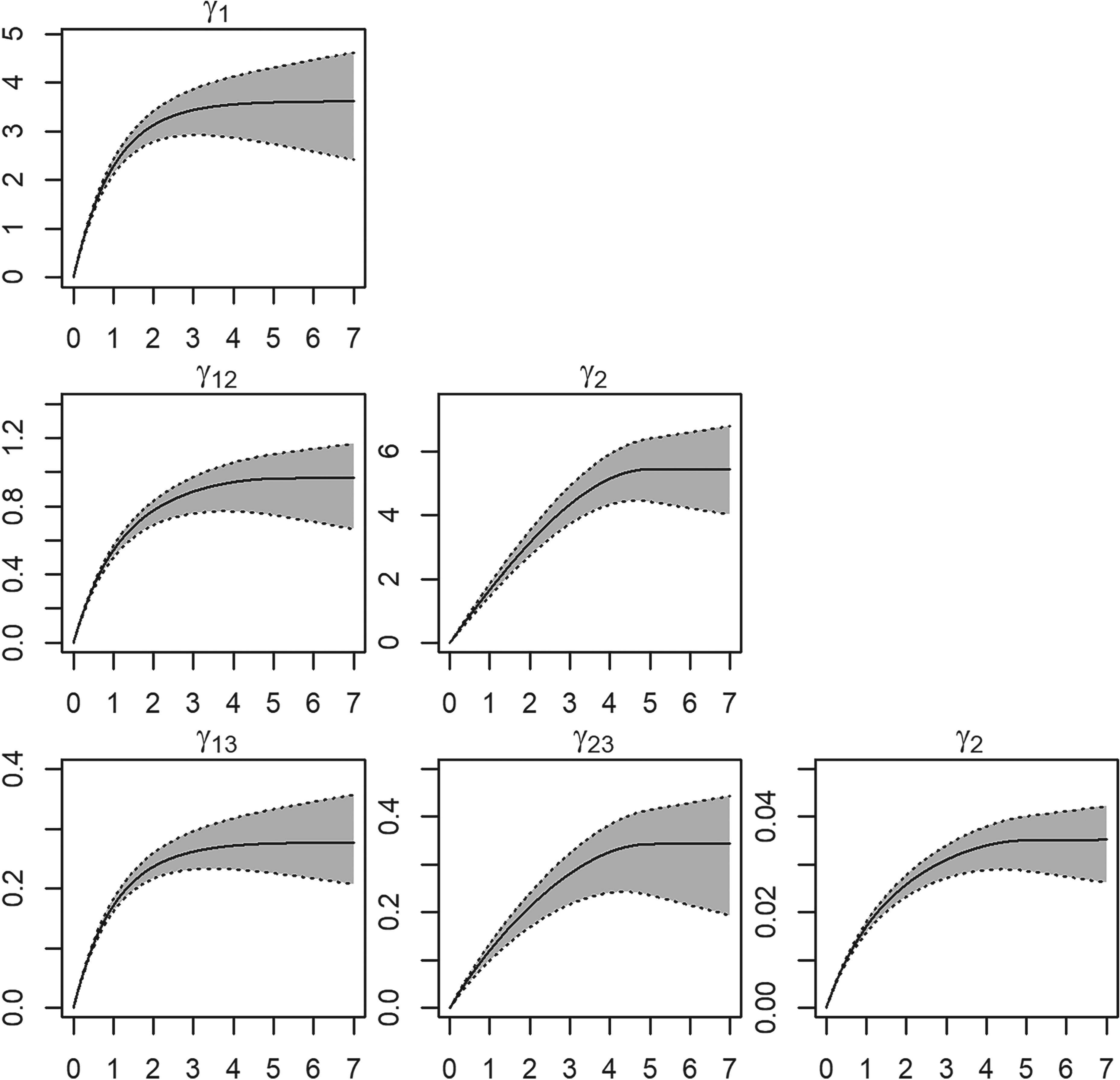
Semivariogram and cross-semivariogram estimation summaries for the 1000 simulated datasets. Average semivariograms estimate (solid line) and “error bandwidths” (gray polygon) with one standard deviation of the semivariogram estimates; the dotted lines represent the lowest and highest deviations from the average estimates.

The sampling variability exhibits both positive and negative fluctuations concerning the true covariance function, with increased variability observed at larger distances. However, at a zero lag distance ( $\mathbf{h}=0$ ), the variability appears to be negligible. A clear inverse relationship between the sampling variability and the strength of spatial association is evident, as greater distances display higher deviations from the average estimates. All semivariograms exhibit a discontinuity at the origin.

3.2.2. Spatial prediction

Poisson cokriging is both a predictive method for estimating the total risk ${\mathcal{R}}_{\ell }({\mathbf{s}}_i)$ at unsampled locations, and a denoising method to generate smoothed maps that accentuate the underlying total risk.

We conducted predictions of the total risk ${\mathcal{R}}_1({\mathbf{s}}_0)$ ( $\mathcal{L}=1$ ) at each prediction location $s_0\in \mathcal{D}=[-10,10]\times [-10,10]$ by using the observed counts of the target and ancillary variables, denoted as $\frac{Y_{\ell i}}{n_{\ell i}}$ when $\ell =1,2,3$ , along with the fitted LMC model as depicted in Figure 2. For each of the 1000 datasets, we estimated ${\mathcal{R}}_1^{*}({\mathbf{s}}_0)$ in different prediction locations. We predicted the total risk ${\mathcal{R}}_1^{*}({\mathbf{s}}_0)$ at 312 unobserved locations, while we employed a leave-one-out validation scheme to smooth the risk values for each of the 625 locations covering $\mathcal{D}$ . We compared the predicted values and smoothed estimates with the true underlying risk ${\mathcal{R}}_1({\mathbf{s}}_0)$ at the corresponding locations.

We compared our results with Poisson kriging using the AE, MSPE, the coverage probability of prediction intervals (95% confidence), and ${\rho }_{\mathcal{R}}$ between the estimated risks and the true risks in the unobserved locations for prediction, and between the smoothed risk and observed risk in the observed locations for smoothing. These comparisons represent the average values obtained from the 1000 simulations.

$$\begin{array}{rl}\text{AE}& =\frac{1}{M}\sum _{m=1}^M\sum _{i=1}^{k_1}(\stackrel{*}{{\mathcal{R}}_1^m}({\mathbf{s}}_i)-{\mathcal{R}}_1^m({\mathbf{s}}_i)),\text{MSPE}=\frac{1}{M}\sum _{m=1}^M\sum _{i=1}^{k_1}(\stackrel{*}{{\mathcal{R}}_1^m}({\mathbf{s}}_i)-{\mathcal{R}}_1^m({\mathbf{s}}_i){)}^2\\ \text{Coverage}& =\frac{1}{M}\sum _{m=1}^M\sum _{i=1}^{k_{\alpha }}\mathbf{1}\{\left|\frac{\stackrel{*}{{\mathcal{R}}_1^m}({\mathbf{s}}_i)-{\mathcal{R}}_1^m({\mathbf{s}}_i)}{\text{MSPE}}\right|<1.96\},{\rho }_{\mathcal{R}}=\frac{1}{M}\sum _{m=1}^M\rho (\stackrel{*}{{\mathcal{R}}_1^m}(\mathbf{s}),{\mathcal{R}}_1^m(\mathbf{s}))\end{array}$$

where $\stackrel{*}{{\mathcal{R}}_1^m}({\mathbf{s}}_i)$ is the estimated value of ${\mathcal{R}}_1^m({\mathbf{s}}_i)$ at location ${\mathbf{s}}_i$ in the $m$ -th simulation for $M=1,2,\dots ,1000$ .

Prediction

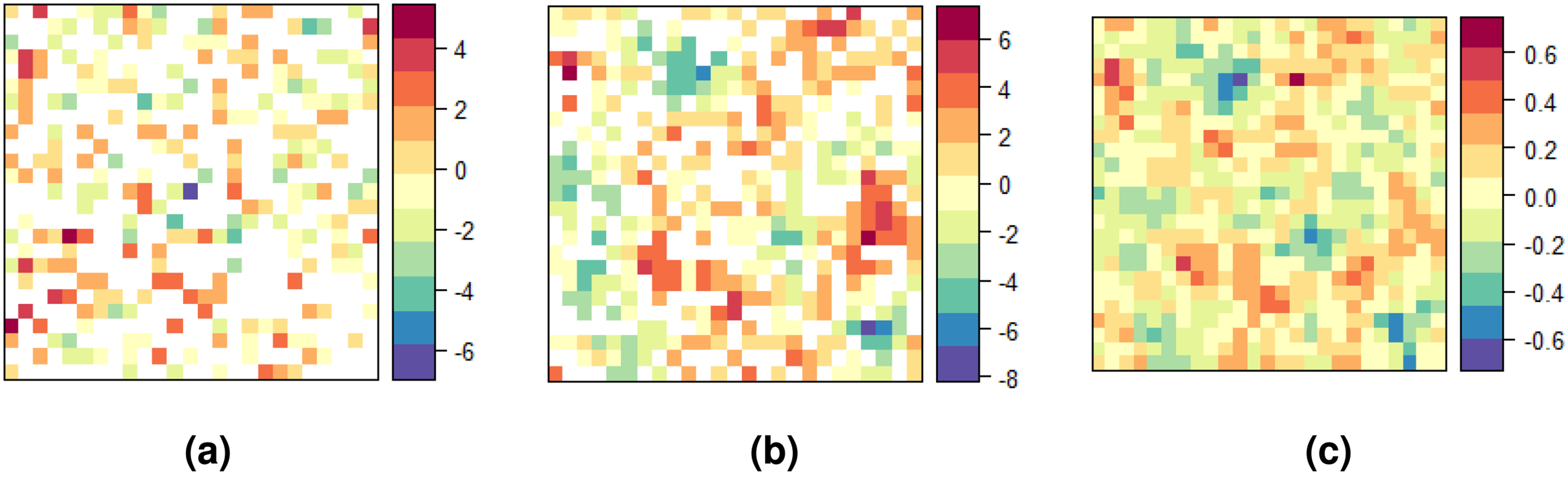
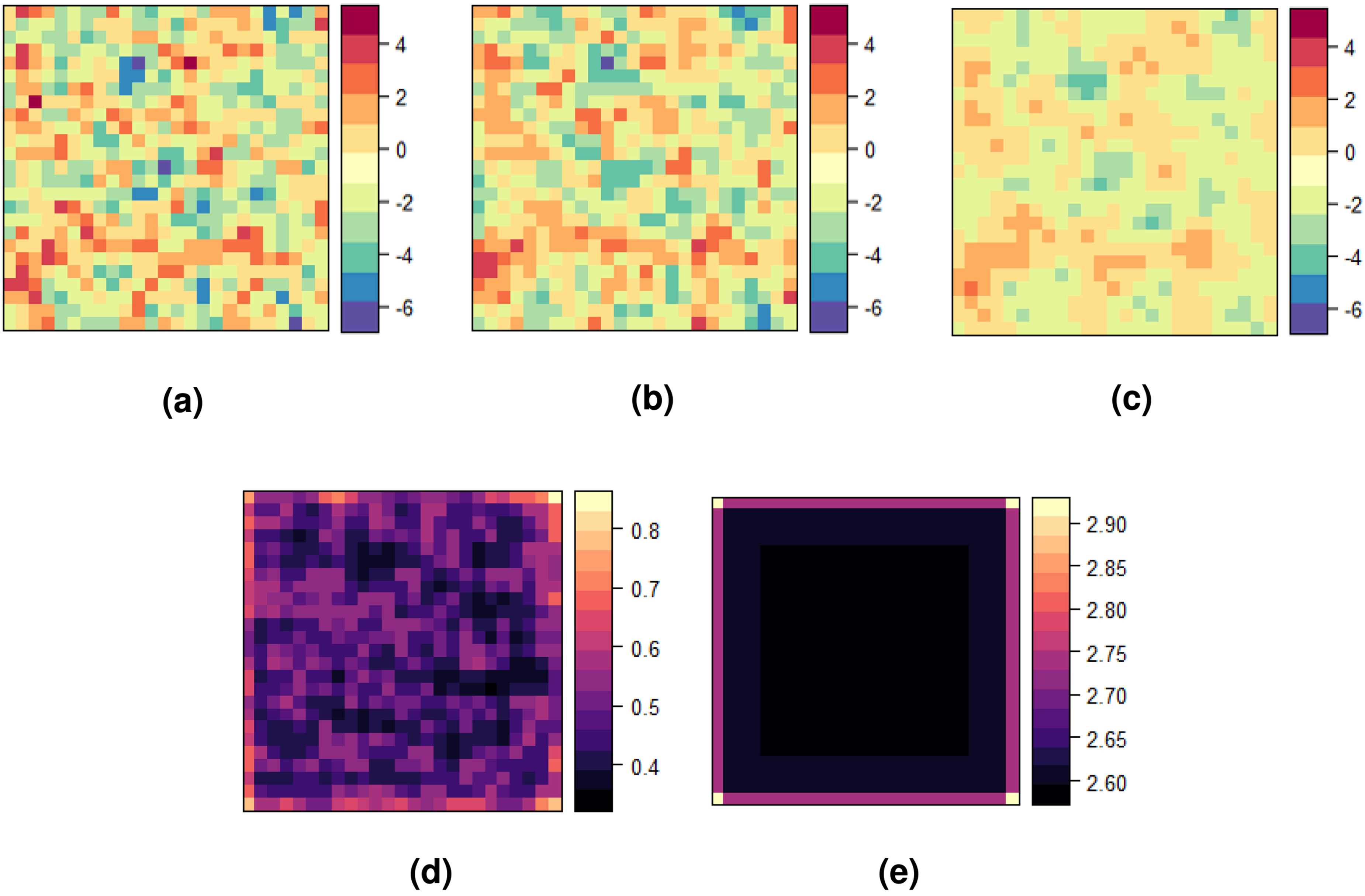
Figure 3 presents the averaged predicted risks at unsampled locations, along with their corresponding variance of the prediction error, for both Poisson cokriging (PCK) and Poisson kriging (PK), in comparison to the underlying risk. The predictions generated by Poisson cokriging (Figure 3(b)) successfully capture both the intensity and spatial patterns of the true risk, while simultaneously attenuating the influence of highly variable risk areas. This result can be attributed to the inclusion of the population sizes in our method, particularly in regions where populations exhibit spatial heterogeneity. Consequently, the resulting predictions display a smoothed pattern that closely resembles the underlying risk distribution, and thus facilitate the visual identification of high and low-risk areas.

Figure 3.

Maps of (a) true total risk log ${\mathcal{R}}_1({\mathbf{s}}_i)$ , (b) predicted total risk log ${\mathcal{R}}_1^{*}({\mathbf{s}}_i)$ , (c) variance of the prediction error ${\sigma }_{\text{ {PCK}}}^2$ for Poisson cokriging (PCK), (d) predicted total risk log ${\mathcal{R}}_1^{*}({\mathbf{s}}_i)$ , and (e) variance of the prediction error ${\sigma }_{\text{ {PCK}}}^2({\mathbf{s}}_i)$ for Poisson kriging (PK) (average of 1000 simulations). (a) $\log {\mathcal{R}}_1({\mathbf{s}}_i)$ ; (b) $\log {\mathcal{R}}_1^{*}({\mathbf{s}}_i)$ (PCK); (c) $\log {\mathcal{R}}_1^{*}({\mathbf{s}}_i)$ (PK); (d) ${\sigma }_{\text{ {PCK}}}^2({\mathbf{s}}_i)$ ; and (e) ${\sigma }_{\text{ {PK}}}^2({\mathbf{s}}_i).$

Poisson kriging (Figure 3(c)) yields over-smoothed predictions in which the risk levels are highly softened. This is particularly evident in the loss of extremely high and low risk values. Its variance map reveals that Poisson kriging exhibits approximately twice the variability compared to PCK. In both models, the confidence of the predictions diminishes as the spatial variability between the risk levels of neighboring cells increases.

The evaluation metrics (Table 1) highlight the superior prediction performance of Poisson cokriging. Specifically, AE, MSPE, and ${\rho }_Y$ consistently favor our method with lower AE and MSPE values and higher correlation with the true values. Despite both Poisson cokriging and Poisson kriging tend to underestimate the risks (as evidenced by the negative average error), the MSPE is approximately 50 $\mathrm{\%}$ smaller for Poisson cokriging. Hence, employing Poisson cokriging leverages auxiliary information to better account for the uncertainty in estimating the risk at unobserved locations. Furthermore, ${\rho }_{\mathcal{R}}$ supports these findings, as it indicates a strong association between the predicted data and the underlying risk.

Smoothing

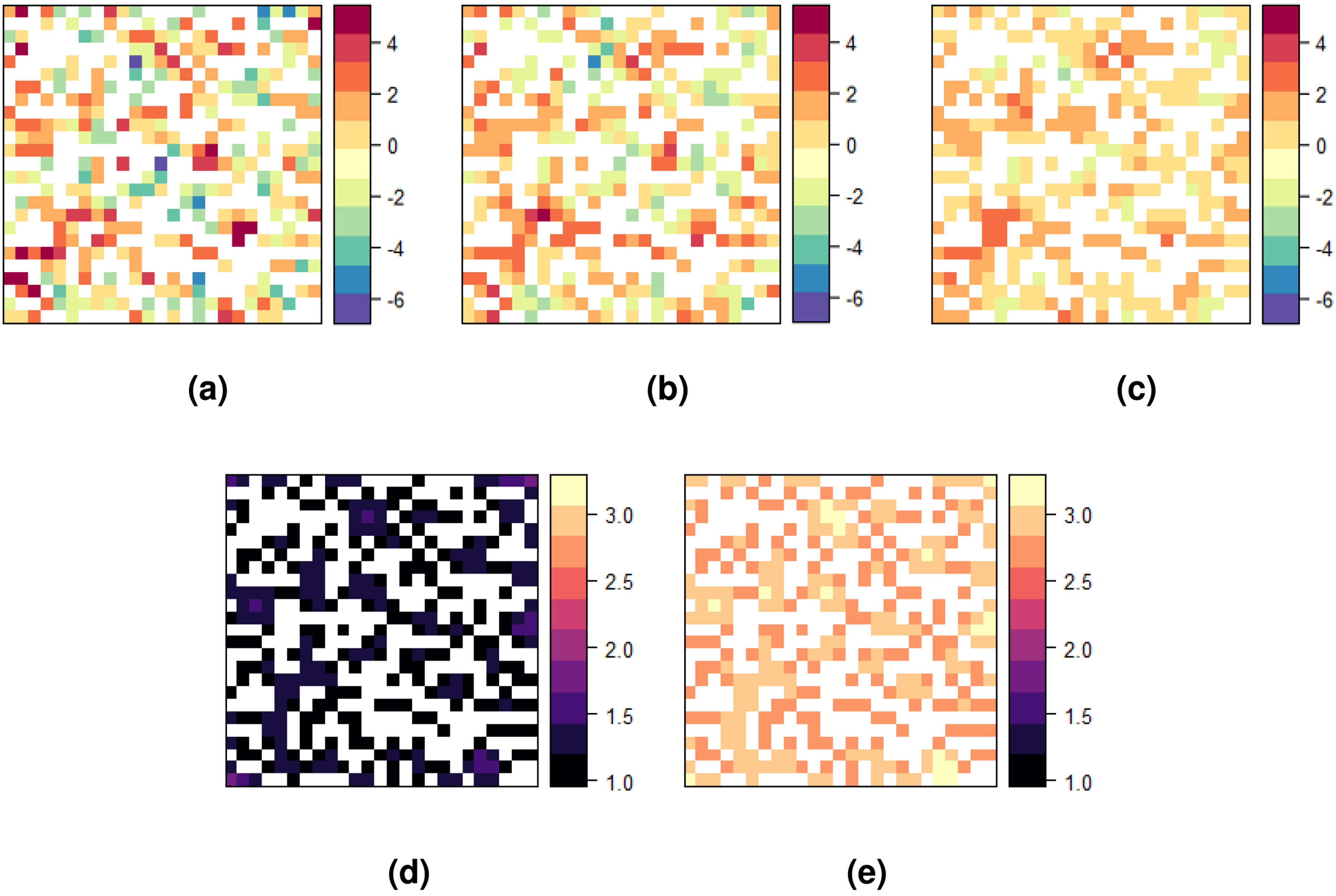
Figure 4 illustrates the averaged smoothed risks across the entire study area, accompanied by the variance of the prediction error. It presents a comparison between the univariate and multivariate versions of Poisson kriging, similar to Figure 3.

Table 1.

Summary assessment metrics to constrain Poisson cokriging and Poisson kriging as predictors for the 1000 simulated datasets.

	Metric
Model	AE	MSPE	${\rho }_{\mathcal{R}}$	Coverage (95%)
Poisson cokriging	$-$ 0.161	1.375	0.831	0.980
Poisson kriging	$-$ 0.275	2.879	0.559	0.941

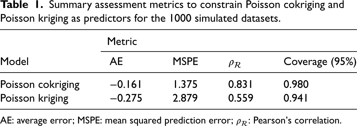
AE: average error; MSPE: mean squared prediction error; ${\rho }_{\mathcal{R}}$ : Pearson’s correlation.

Figure 4.

Maps of (a) the observed total risk log $({\hat{Y}}_{1i}/n_{1i})$ , (b) smoothed total risk log ${\mathcal{R}}_1^{*}({\mathbf{s}}_i)$ , (c) variance of the prediction error ${\sigma }_{\text{ {PCK}}}^2$ for Poisson cokriging (PCK), (d) smoothed total risk log ${\mathcal{R}}_1^{*}({\mathbf{s}}_i)$ , and (e) variance of the prediction error ${\sigma }_{\text{ {PCK}}}^2({\mathbf{s}}_i)$ for Poisson kriging (PK) (average of 1000 simulations). (a) $\log ({\hat{Y}}_{1i}/n_{1i})$ ; (b) $\log {\mathcal{R}}_1^{*}({\mathbf{s}}_i)$ (PCK); (c) $\log {\mathcal{R}}_1^{*}({\mathbf{s}}_i)$ (PK); (d) ${\sigma }_{\text{ {PCK}}}^2({\mathbf{s}}_i)$ ; and (e) ${\sigma }_{\text{ {PK}}}^2({\mathbf{s}}_i)$ .

The smoothed map produced by Poisson cokriging (Figure 4(b)) provides a denoised representation of the observed sample counts ( $Y_{1i}/n_{1i}$ ), closely resembling the true underlying risk pattern (Figure 4(a)). This filtering enables the easy identification of hotspots and coldspots, allowing for clear distinctions between high-risk and low-risk areas throughout the study region. Moreover, the overall range of the underlying risk is well preserved. As in the prediction results, Poisson kriging has a pronounced smoothing effect, leading to a loss of local variations, despite the preservation of main risk areas. The variance maps demonstrate an enhanced accuracy in the presence of auxiliary information. Specifically, the variance associated with Poisson kriging is three times higher as compared to our proposed method, and it is uniformly distributed across the study area. This indicates that the variance fluctuations are relatively small from one cell to another. The variance map for Poisson cokriging exhibits its highest values in cells where high and low risks interact, suggesting increased uncertainty in these transitional regions.

Table 2 summarizes the assessment metrics for Poisson cokriging and Poisson kriging as smoothers based on the 1000 simulated datasets. For Poisson cokriging, the average error is close to zero, indicating a low bias in the risk estimation. The MSPE value equals 1.530, suggesting a relatively low prediction error. Furthermore, the ${\rho }_{\mathcal{R}}$ value shows a strong association between the predicted risks and the actual underlying risks. In contrast, Poisson kriging exhibits a slightly negative AE value equal to $-$ 0.001, suggesting a slight underestimation of the risks. The MSPE value is almost twice as high as that of Poisson cokriging. The ${\rho }_{\mathcal{R}}$ shows a weaker association between the predicted risks and the true underlying risks as compared to our model.

Table 2.

Summary assessment metrics to constrain Poisson cokriging and Poisson kriging as smoothers for the 1000 simulated datasets.

	Metric
Model	AE	MSPE	${\rho }_{\mathcal{R}}$	Coverage (95%)
Poisson cokriging	0.000	1.530	0.774	0.971
Poisson kriging	$-$ 0.001	2.848	0.524	0.925

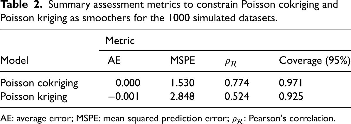
AE: average error; MSPE: mean squared prediction error; ${\rho }_{\mathcal{R}}$ : Pearson’s correlation.

3.2.3. Computational time

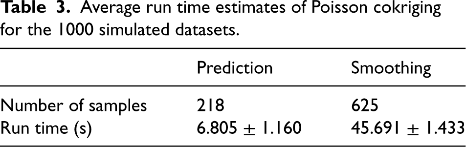
Evaluating the computational efficiency of a modeling approach is crucial, especially in scenarios where real-time performance or the analysis of large datasets is required. In this simulation study, we assessed the computational time of the Poisson cokriging method for both prediction and smoothing processes.

Table 3 presents the average run time estimates in seconds (s) for the 1000 simulated datasets. The smoothing process (0.031 s/sample), naturally, is more computationally intensive than the prediction process (0.072 s/sample). This result is expected due to the iterative removal of observed data points, covariance matrix re-calculation and risk estimation involved in smoothing the disease rates. Nonetheless, the running times, even for the smoothing process, remain reasonably short, with standard deviations of < 2 s.

Table 3.

Average run time estimates of Poisson cokriging for the 1000 simulated datasets.

	Prediction	Smoothing
Number of samples	218	625
Run time (s)	6.805 $\pm$ 1.160	45.691 $\pm$ 1.433

While the computational cost of spatial modeling techniques can be influenced by various factors, such as the number of samples, the complexity of the spatial dependence structure, and the available computational resources (e.g. CPU, RAM, and parallelization capabilities), our results demonstrate that Poisson cokriging exhibits efficient performance in both prediction and smoothing with a moderate sample size of 625 observations. Since disease risk estimation is typically performed for geographical units, and large datasets are relatively rare at the areal level, these computational time estimates for Poisson cokriging are promising and suggest its suitability for practical applications in the field of disease risk assessment.

4. Application to HIV incidence in Pennsylvania, the United States

In the United States (U.S.), the prevalence of these STDs remains a concern. According to data from the Centers for Disease Control and Prevention (CDC), rates of HIV, gonorrhea, and chlamydia disproportionately affect marginalized groups such as racial/ethnic minorities, gay, and bisexual men, youth, and lower income populations. ²⁵ While southern states present the highest rates overall, Pennsylvania remains above national averages, with over 1000 new HIV diagnoses in 2019 in cities like Philadelphia and Pittsburgh. Stigma and insufficient screening persist in enabling these syndemics, though data suppression further obscures the true burden. To protect privacy, HIV/STD data with low-counts or vulnerable groups is often restricted, limiting statistical reliability. ²⁶ While ethically justified, this constrains public health capacity.

Leveraging data on correlated STDs like gonorrhea and chlamydia could help estimate geographic HIV burden where direct data is limited or missing. As these STDs are highly correlated, their incidence provides information about unobserved HIV risk and improves representation beyond what constrained surveillance data can directly capture.^5,9 Research shows that in the context of HIV, gonorrhea, and chlamydia is important. Co-infection with gonorrhea or chlamydia can increase HIV susceptibility 2–5 fold during exposure due to genital inflammation and higher viral load in genital secretions,^27,28 and geographic research reveals substantial overlaps between populations affected by HIV and these other STDs.^29–31 Those with the highest HIV rates often have high gonorrhea and chlamydia burdens as well, concentrated in marginalized groups facing healthcare access barriers, stigma, poverty, and heightened behavioral risks like multiple partners or commercial sex work.^32,33 These social and structural vulnerabilities create geographic hotspots where HIV, gonorrhea, and chlamydia are syndemic.

To analyze HIV incidence in Pennsylvania, we used 2021 data on HIV, chlamydia, and gonorrhea incidence and HIV prevalence from the 66 counties of Pennsylvania (excluding Philadelphia county). We include the HIV prevalence data as an auxiliary variable as it shares similar pattern with the HIV incidence data. The data came from the STD Surveillance System managed by the CDC. While the cases and population data were aggregated at the state-level, some state-level data were suppressed or undisclosed, particularly for HIV.

To address the data absence and unreliability, we will use the method described above. The high degree of overlap between gonorrhea, chlamydia, and HIV makes them suitable for synergistic modeling. Poisson cokriging incorporates the auxiliary gonorrhea and chlamydia data to estimate HIV prevalence in unmeasured locations. Also, it filters noise in the observed data, producing improved representations of Pennsylvania’s underlying HIV risk surface compared to using the sparse surveillance data alone. Applying Poisson cokriging facilitates more accurate HIV burden estimates and helps to fully characterize Pennsylvania’s epidemic given constraints around existing public health data.

Preliminary analysis showed that Philadelphia’s STDs data exhibited high variance and did not correlate—spatially—well with other counties, so it was excluded to reduce noise and improve signal detection.

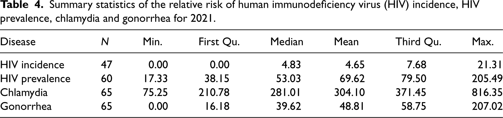
Table 4 and Figure 5 show summary statistics and spatial distribution of STDs risk across counties. HIV incidence risk ranged from 0 to 21.3 per 100,000 inhabitants, though this interval is unreliable given 30% suppressed data. HIV prevalence oscillated between 1.33 and 233 in 2021. Chlamydia and gonorrhea risk ranged from 1 to 816.30 and 0 to 207.00, respectively. Spatial distribution was similar for southeastern and northwestern counties, while central county risk differed across diseases.

Figure 5.

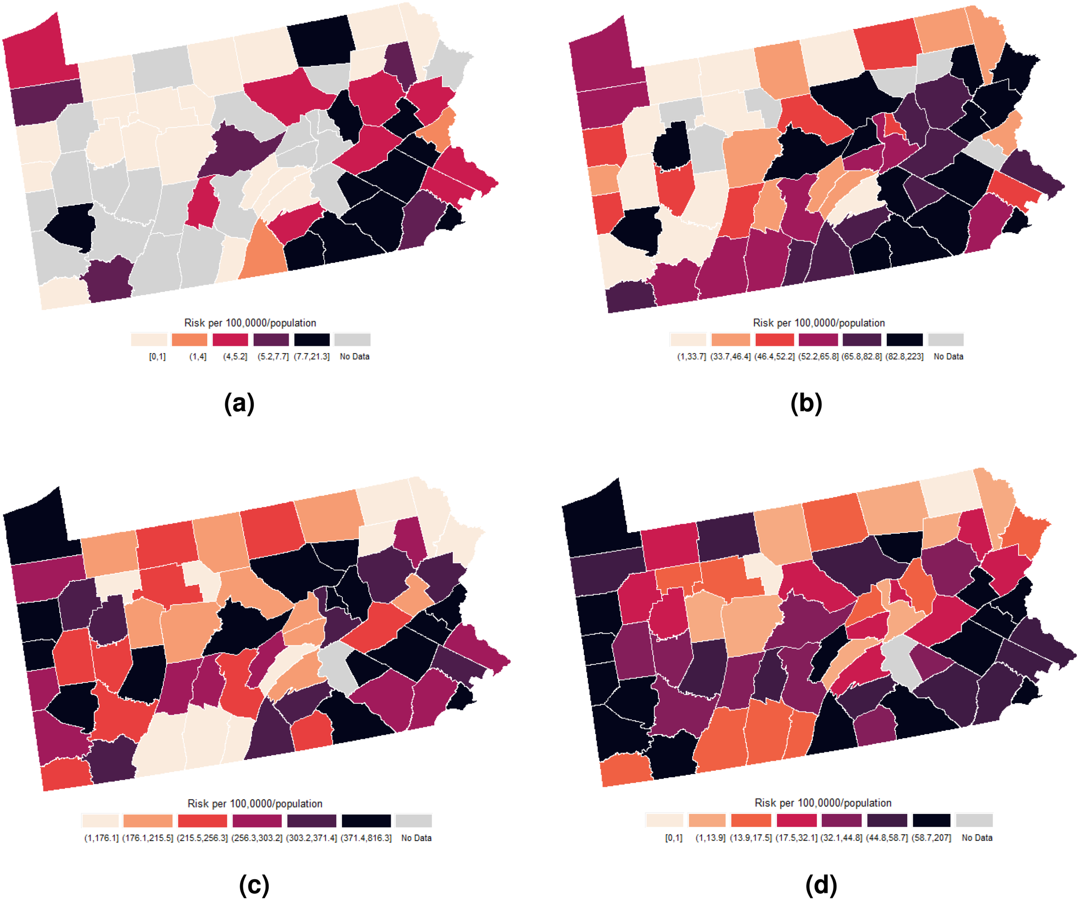
Spatial distribution of the sample risks of human immunodeficiency virus (HIV) incidence, HIV prevalence, chlamydia, and gonorrhea for Pennsylvania in 2021. (a) HIV incidence; (b) HIV prevalence; (c) chlamydia incidence; and (d) gonorrhea incidence.

Table 4.

Summary statistics of the relative risk of human immunodeficiency virus (HIV) incidence, HIV prevalence, chlamydia and gonorrhea for 2021.

Disease	N	Min.	First Qu.	Median	Mean	Third Qu.	Max.
HIV incidence	47	0.00	0.00	4.83	4.65	7.68	21.31
HIV prevalence	60	17.33	38.15	53.03	69.62	79.50	205.49
Chlamydia	65	75.25	210.78	281.01	304.10	371.45	816.35
Gonorrhea	65	0.00	16.18	39.62	48.81	58.75	207.02

4.1. Modeling of the spatial structure

We computed the empirical semivariogram and cross-semivariogram defined by (12) and (13) under the assumption of isotropy. Rather than using the geographical centroids of each county, we calculated the semivariograms using population-weighted centroids. This provided a more reliable representation of the proximity structure within Pennsylvania counties. Population census data at the census tract level ³⁴ were leveraged to determine the weighted centroids.

Figure 6 shows the estimated semivariograms and their fitted theoretical models. We fitted a stable model with zero nugget effect by least squares. While the semivariogram plots suggest a potential nugget effect, the lack of semivariance estimates for county pairs at short distances ( $d<$ 45 km) made this conclusion questionable. Additionally, the linear model did not converge with a nugget effect included.

Figure 6.

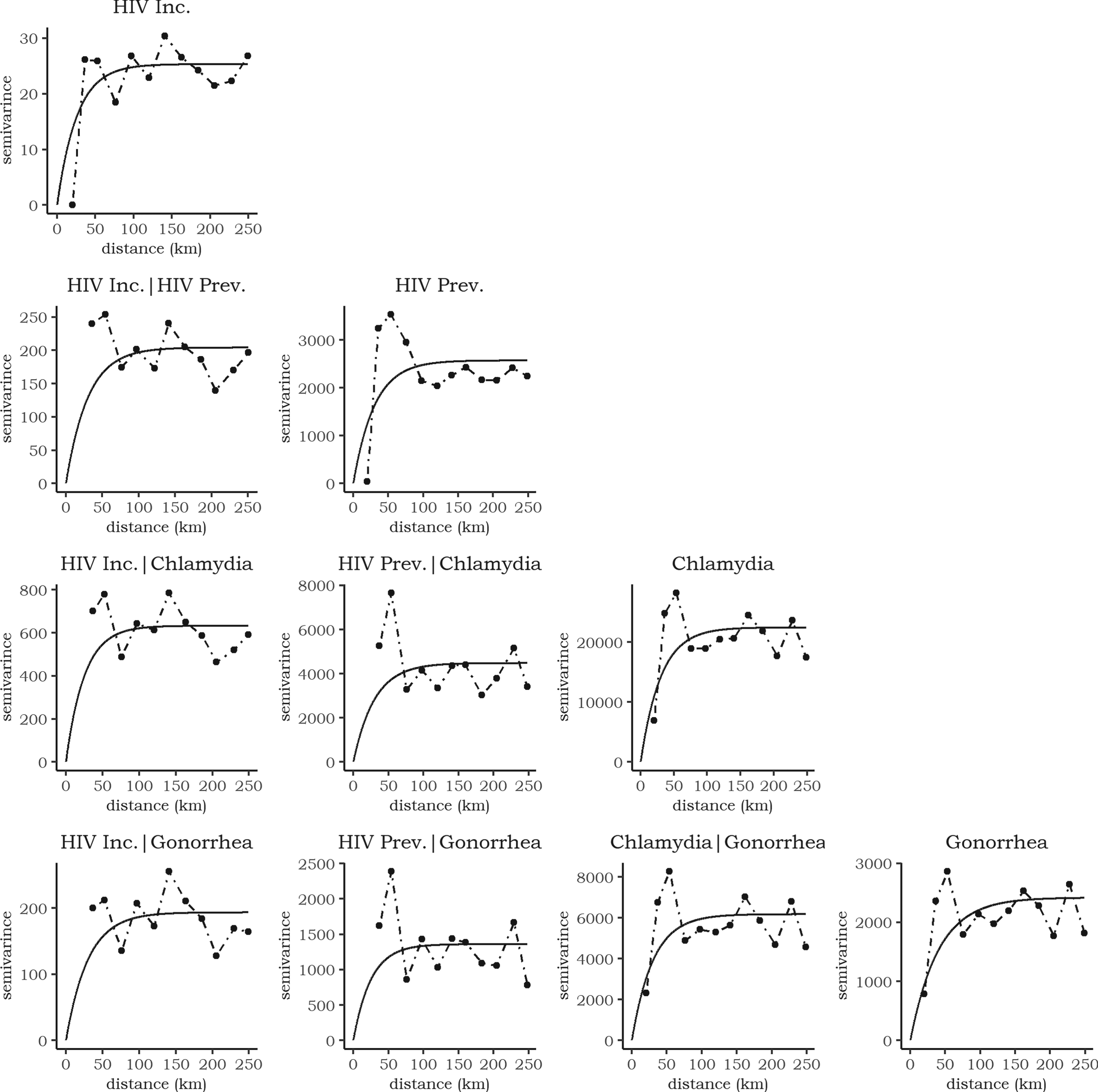
Empirical (points) and fitted (black line) semivariogram and cross-semivariogram for the four sexually transmitted diseases (STDs). The dashed lines connect the empirial estimates.

High semivariance values at the second and third lags resulted from two factors: the limited observations at these distances and the high STD risk in Pittsburgh. Subsequent semivariance values stabilized as the number of observations increased. Most point estimates were biased due to data overdispersion, but the semivariogram and cross-semivariogram fits were satisfactory. The HIV incidence semivariograms showed the lowest variability, indicating shared spatial processes with other STDs. Chlamydia risk displayed high spatial variability, with notable differences compared to other diseases.

The sills ranged from 25.5 to 22440.5, with HIV incidence having the smallest and chlamydia the highest sill. The effective ranges were 25.8–66.6 km, suggesting that spatial correlations were local, occurring between counties and their immediate neighbors. The smoothness parameters of the stable model ranged from 1.2 to 1.7, meaning the semivariograms were close to exponential (smoothnes of 1) or Gaussian (smoothness of 2) models.

4.2. Cokriging of the HIV incidence

We performed prediction and smoothing to estimate HIV incidence risk. For counties with suppressed data, we predicted risk values. By predicting values for counties with missing information, we can conduct a comprehensive analysis across the entire state of Pennsylvania. This ensures that no geographic regions are excluded, which could lead to an incomplete understanding of the spatial patterns and drivers of the HIV incidence. For counties with available data, we smoothed the risk values. Smoothed risk values account for the spatial dependence structure and reduce the impact of local noise and outliers in the data. HIV prevalence, chlamydia, and gonorrhea risks were used as auxiliary variables to improve the cokriging estimates.

Figure 7(a) shows the smoothed map of estimated HIV incidence risk after integrating the predicted and filtered values. The map reveals spatial clustering of high HIV incidence rates in Pennsylvania’s densely populated southeastern and northwestern counties. The top four counties—Allegheny, Delaware, Montgomery, and Chester—account for 46% of the state’s population and 58.7% of diagnosed infections, besides Philadelphia. Urbanization appears to be a key driver, as these counties encompass major metropolitan hubs like Pittsburgh. Proximity to cities has been associated with higher HIV transmission, potentially due to factors like poverty, drug use, and stigma facing marginalized groups. ²⁵

Figure 7.

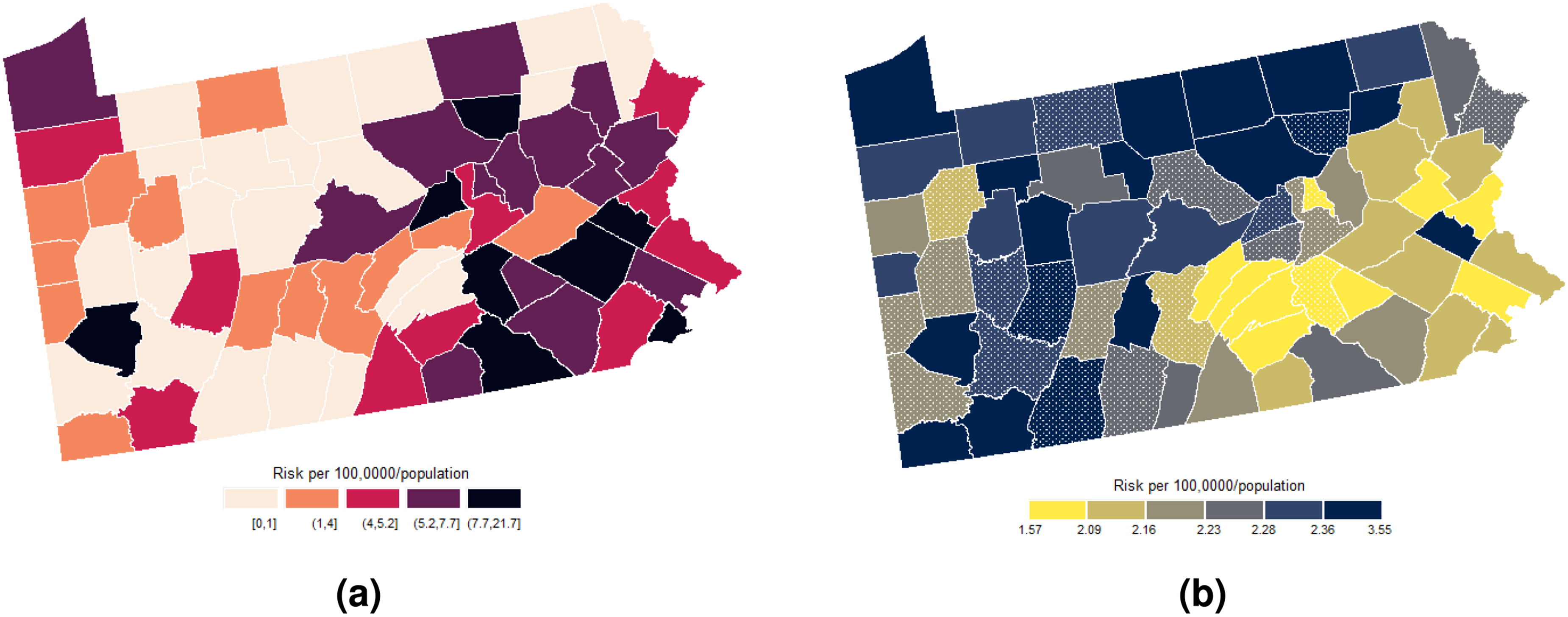
(a) Spatial distribution of the predicted and smoothed risks of human immunodeficiency virus (HIV) incidence and (b) its corresponding prediction error variance. The dotted polygons represent the prediction counties. (a) prediction and (b) variance.

Beyond urbanization, limited healthcare access also correlates with increased incidence. Counties such as Lehigh, Cambria, Jefferson, and Fayette with the high HIV rates have disproportionately high rates of uninsured individuals, constraining prevention and treatment. ³⁵ Systemic disparities also manifest geographically—counties like Bucks, Delaware, and Erie with large African American populations face higher incidence stemming from social stigmas and inequalities. ³⁶

High pre-exposure prophylaxis prescription rates across counties intended to prevent HIV transmission correspond to spikes in incidence, suggesting risk compensation behaviors may be occurring. ³⁷ Furthermore, overlapping high rates of fatal and nonfatal overdoses indicate links between injection drug use and transmission. ²⁵

In contrast, lower incidence clusters in rural counties across southeastern and southcentral Pennsylvania like Huntingdon, Juniata, Mifflin, and Fulton counties. These regions tend to have lower population densities, higher insurance coverage, and less presence of marginalized groups. Clusters of high incidence in specific counties, however, highlight the need for targeted prevention efforts and resources to mitigate disparities. Further research on sociogeographic drivers is as well warranted.

Figure 7(b) displays the cokriging variance map. The cokriging variance map serves as an uncertainty map, quantifying the prediction error variance as measures of spatial uncertainty. The cokriging variance can be used as the corresponding prediction/smoothing variance as it reflects the uncertainties in the estimated risk surface, considering the spatial dependence structure and the relationships with auxiliary variables.

Overall, variances tend to be lower in counties with smoothed risk estimates as compared to those with predicted estimates. Counties with few immediate neighbors, such as those along state boundaries such as Erie, Potter, Tioga, and Bradford, exhibit higher variances. This reflects the spatial influence structure defined by between-county semivariances. Since Poisson cokriging modulates population size effects, variances tend to be inversely proportional to county populations—densely populated counties have smaller variances. Uncertainty also appears problematic in “low-count neighborhoods,” that is, counties surrounded by areas with very low or zero observed HIV risk, such as Brandford, Fayette, and Forest.

The spatial configuration of counties and the sampling pattern govern variance through the modeled dependence structure. Less inter-county dependence and fewer observations produce greater prediction uncertainty. Variance stabilization occurs in more densely sampled areas and for counties nearer to neighbors with data (such as the southeastern counties), as more information is shared through spatial smoothing.

The map in Figure 7(b) thus reveals the geography of reliability, highlighting counties requiring additional sampling, complementary data, or closer inspection while conveying spatially structured confidence in the estimated HIV incidence risk surface. In this sense, the HIV incidence risk estimates for southeastern counties like Bucks, Montgomery, Delaware, and Northampton have higher reliability. Direct application of preventive and control public health measures is therefore suggested. Conversely, counties in the northeastern region such as Potter, Tioga, Bradford, and Sullivan demand further examination before implementing policies, given their greater uncertainty.

The variance map, in the context of the HIV epidemics in Pennsylvania, provides a crucial spatial context for informed decision-making and efficient resource allocation for the local public health practice. It indicates where available HIV estimates per each county may be directly usable versus counties that would benefit from additional sampling or validation. It can also guide future data collection strategies and resource allocation for surveillance and reporting in areas with greater uncertainty.

4.3. Assessment of Poisson cokriging

To quantitatively evaluate and compare the predictive performance of the Poisson cokriging and kriging models fitted to the Pennsylvania HIV incidence data, we used the assessment metrics described in Section 3.2.2 except the coverage probability for $M=1$ , since we only get one estimation for the data. The assessment metrics were computed by comparing the smoothed risk estimates against the observed risk values. This approach is analogous to leave-one-out cross-validation, as the smoothing process inherently involves the exclusion of the observed risk value at each location during the estimation procedure. We included as well the maximum kriging variance (max( ${\sigma }_{\text{ {PCK}}}^2$ )) to evaluate the reliability of the HIV incidence estimates by measuring the prediction uncertainty.

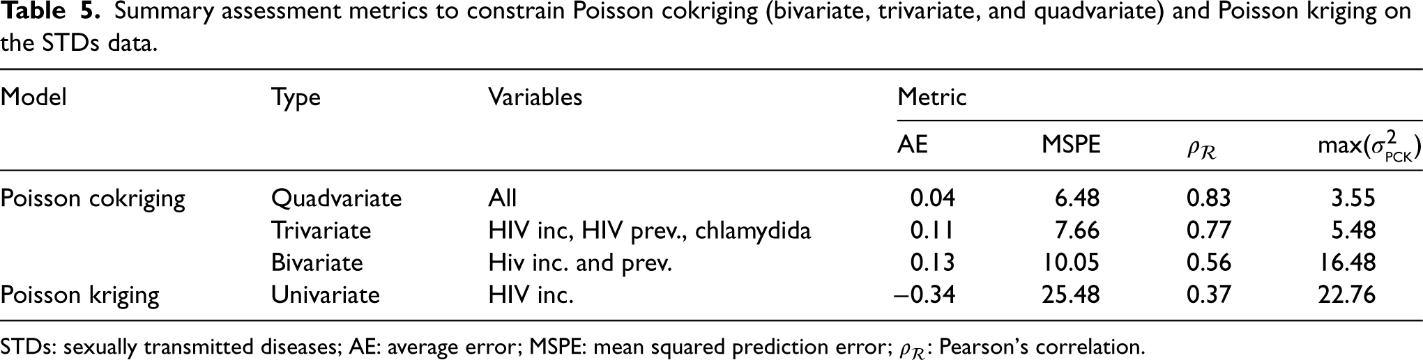
The assessment metrics for Poisson cokriging (bivariate, trivariate, and quadvariate) and Poisson kriging are presented in Table 5. Univariate Poisson kriging, which disregards auxiliary information, exhibits the poorest outcomes across all metrics with a MSPE value equal to 25.48, a correlation coefficient of 0.37 between observed and smoothed values, and high kriging variance of 22.76. Incorporating additional correlated covariates through multivariate Poisson cokriging markedly improves predictive accuracy and uncertainty quantification. The predictive accuracy reflects the similarity between the estimated values and the true values considering the inherent uncertainties arising from the modeling process and the noise present in the observed data, while the uncertainty quantification provides an assessment of the reliability of the predictions.

Table 5.

Summary assessment metrics to constrain Poisson cokriging (bivariate, trivariate, and quadvariate) and Poisson kriging on the STDs data.

Model	Type	Variables	Metric
			AE	MSPE	${\rho }_{\mathcal{R}}$	max( ${\sigma }_{\text{ {PCK}}}^2$ )
Poisson cokriging	Quadvariate	All	0.04	6.48	0.83	3.55
	Trivariate	HIV inc, HIV prev., chlamydida	0.11	7.66	0.77	5.48
	Bivariate	Hiv inc. and prev.	0.13	10.05	0.56	16.48
Poisson kriging	Univariate	HIV inc.	-0.34	25.48	0.37	22.76

STDs: sexually transmitted diseases; AE: average error; MSPE: mean squared prediction error; ${\rho }_{\mathcal{R}}$ : Pearson’s correlation.

The bivariate model, leveraging both HIV incidence and HIV prevalence variables, reduces the MSPE by over 60% and increases correlation to 0.56. The trivariate approach further decreases the MSPE to 7.66 and improves correlation to 0.77 by also incorporating the chlamydia data. Finally, the quadvariate cokriging model, which additionally uses gonorrhea incidence, provides optimal performance as evidenced by the lowest MSPE and average error alongside the highest correlation.

Table 6 presents the running time estimates in seconds for the four Poisson cokriging cases, where we predicted and smoothed the HIV risk for the 66 counties of the study case. As more diseases are incorporated into the analysis, the running time increases for both prediction and smoothing processes. However, the incremental increase in running time is relatively small when adding additional diseases. For instance, despite the added complexity, the running time for quadvariate prediction (0.458 s) is only marginally higher than the bivariate case (0.200 s).

Table 6.

Run time estimates in seconds (s) of Poisson cokriging (univariate, gbivariate, trivariate, and quadvariate) on the sexually transmitted diseases (STDs) data.

Type	Run time (s)
	Prediction	Smoothing
Quadvariate	0.458	1.208
Trivariate	0.316	0.793
Bivariate	0.200	0.233
Univariate	0.110	0.184

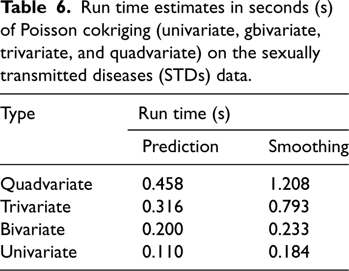
The smoothing process generally has a larger computational burden than the prediction process. Nevertheless, even in the computationally more demanding quadvariate case, the smoothing time cost (1.208 s) remains reasonably low.

Althought the running time raises when introducing more diseases into the modeling framework, prediction accuracy also improves (Table 5). This trade-off between computational cost and data richness must respond to the specific needs of the analysis. For time-critical applications requiring rapid predictions, lower-order models, such as the univariate or bivariate cases, may be preferred due to their shorter computational times. Conversely, in scenarios where maximizing prediction accuracy is the primary objective, the quadvariate model may be the most suitable choice, despite its slightly longer running time.

5. Disscusion

In this article, we addressed the challenges associated with multivariate geostatistical modeling of disease count data and introduced a generalized version of Poisson cokriging, presented by Payares-Garcia et al. ⁵ for the prediction and smoothing of spatial disease counts. Our method builds upon pair-wise correlations between a target variable and other ancillary variables exemplified as spatial counts, enabling the modeling of complex spatial dependencies and the incorporation of auxiliary information.

By means of a simulation analysis, we demonstrated the effectiveness of Poisson cokriging in accurately estimating disease risk and producing smoothed risk maps that capture fine-scale variations in disease occurrence. Compared to Poisson kriging, it showed superior prediction performance, with smaller MSPE values and higher ${\rho }_Y$ values with the true underlying risk. The smoothing capabilities of Poisson cokriging also outperformed Poisson kriging, providing denoised representations of disease counts that closely resembles the true risk pattern.

Poisson cokriging proved to be a valuable spatial modeling tool for estimating and mapping disease risk in practical settings. By incorporating auxiliary information from correlated variables like chlamydia and gonorrhea incidence, the multivariate approach borrowed strength and improved characterization of the complex incidence patterns of HIV incidence risk across Pennsylvania counties. The Poisson cokriging model integrating four STDs variables achieved the best prediction error and correlation between observed and predicted HIV incidence. Cross-validation confirmed the superiority of cokriging over univariate Poisson kriging, with accuracy gains of over 50% for multiple metrics. The enhanced predictions quantify and visualize local HIV hotspots, while the uncertainty estimates delineate regions requiring additional sampling and screening. Overall, Poisson cokriging leveraged spatial multivariate dependence to generate reliable, high-resolution HIV incidence risk estimates from sparse, incomplete public health surveillance data. The methodology could be easily applied to prediction and mapping of disease rates in other settings.

Our findings underscore the potential of Poisson cokriging for disease mapping and surveillance. By leveraging the multivariate nature of disease counts and incorporating auxiliary information, it offers meaningful and richer risk predictions, a better depiction of spatial interdependencies, and enhanced identification of high-risk and low-risk areas. Moreover, it holds promise in elucidating the existence of shared risk factors and uncovering unknown associations between diseases. Likewise, integrating uncertainty visualization with disease mapping enables making data-driven decisions tuned to local reliability. This allows public health officials to target efforts where impact can be maximized based on the spatial structure of confidence in the model outputs. These advantages make Poisson cokriging a promising method for public health research and decision-making, supporting the development of targeted interventions and resource allocation strategies. Whilst multivariate Poisson cokriging is developed to deal with epidemiological data, given its nature, it can be extended to other domains such as economy, biology, and ecology, in which dependence between count variables is also spatially located.

Poisson cokriging still requires further enhancements to realize its full potential in multivariate disease mapping applications. Currently, it exclusively accommodates positive spatial correlations among disease counts. A future extension of our method will incorporate negative spatial correlations as well. This phenomenon has been documented by Li et al., ³⁸ Yii et al., ³⁹ and Sayar et al. ⁴⁰ Another avenue for advancement lies in the inclusion of non-count auxiliary variables. Introducing ancillary data in the form of risk factors will not only enrich the prediction process but also downscale the risk when high-resolution data are available. Further research could explore integrating socioeconomic and demographic covariates to potentially improve representations of the complex multivariate processes driving disease transmission. Incorporating space-time observations might as well advance Poisson cokriging understanding of the spatial-temporal character of diseases. This extension might offer further insights into disease incidence, prevalence, and distribution, which are crucial in detecting emerging outbreaks, assessing the effectiveness of interventions, and monitoring disease control measures. ⁴¹ Another step is appropriately accounting for the variable support, as Goovaerts ⁹ suggested. The implementation of multivariate Poisson cokriging up to four variables in the form of R code can be found at https://github.com/DavidPayares/Poisson-cokriging-multivariate.