Unsupervised Liu-type shrinkage estimators for mixture of regression models

Abstract

The mixture of probabilistic regression models is one of the most common techniques to incorporate the information of covariates into learning of the population heterogeneity. Despite its flexibility, unreliable estimates can occur due to multicollinearity among covariates. In this paper, we develop Liu-type shrinkage methods through an unsupervised learning approach to estimate the model coefficients in the presence of multicollinearity. We evaluate the performance of our proposed methods via classification and stochastic versions of the expectation-maximization algorithm. We show using numerical simulations that the proposed methods outperform their Ridge and maximum likelihood counterparts. Finally, we apply our methods to analyze the bone mineral data of women aged 50 and older.

1. Introduction

As a bone metabolic disease, osteoporosis is characterized when the mineral density of bone tissues decreases significantly, leading to various major health problems such as skeletal fragility and osteoporotic fractures. These can occur in different body areas, including the hip, spine, and femur.^1,2 Bone mineral density (BMD) is considered one of the most reliable predictors in determining osteoporosis status. ³ For example, approximately every 1 out of 3 women and 1 out of 5 men aged 50 and older have osteoporosis and its fractures. ⁴ Osteoporosis typically occurs without any significant symptoms. In South Korea, for example, almost 75% of patients are unaware of their osteoporosis problem. ⁵ BMD score of an individual improves until age 30 and declines as the individual ages. As the aged population is growing, it is essential to study osteoporosis to plan the well-being and life quality of the aged groups of the communities.

BMD values are measured through dual-energy X-ray absorptiometry imaging and require a costly and time-consuming procedure. Unlike BMD scores, clinicians have access to various easily attainable explanatory variables about patients, including BMI, weight, age, and test results from previous years. Linear regression models are well-known statistical tools to investigate the impact of a set of covariates (e.g. patients’ characteristics) on a response variable (e.g. BMD measurement). The least squares (LSs) method is a common method for estimating the regression model coefficients; however, the LS method can lead to extremely unreliable and misleading results in multicollinearity when the covariates are linearly dependent. As a shrinkage method, Ridge regression is a common solution to the multicollinearity problem. A small ridge parameter is not enough to handle the ill-conditioned design matrix when the problem is severe. On the other hand, large values of the ridge parameter render more biases in the estimation. The Liu-type (LT) shrinkage method was proposed in the work of Liu ⁶ to address the multicollinearity and was extended in the work of Duran et al. ⁷ to the semi-parametric regressions. Later on, the Stein-rule LT estimators for elliptical regression models was developed in the work of Arashi et al. ⁸ and properties of rank-based samples was used in the work of Pearce and Hatefi ⁹ to improve the LT shrinkage estimators for linear and logistic regressions.

Finite mixture models (FMMs) are probabilistic model-based tools to analyze heterogeneous populations. The maximum likelihood (ML) method is one of the most popular techniques for estimating the parameters of the FMMs. A part of the popularity comes from the expectation-maximization (EM) algorithm ¹⁰ that enables computing the ML estimates of the FMMs. The EM algorithm decomposes the ML estimation procedure into E- and M-steps and iteratively estimates the parameters of the FMMs. Stochastic EM (SEM) algorithm ¹¹ was developed as a stochastic teacher of the probabilistic EM algorithm for mixture models. Also, Celeux and Govaert ¹² proposed a classification EM (CEM) algorithm in which a classification step is implemented in the iteration for maximization based on classified data. The mixture of regression models ¹³ incorporates the properties of the FMMs into linear regression models. The ML and EM algorithms to fit a mixture of regression models was investigated in the work of Faria and Soromenho ¹⁴ , Hawkins et al. ¹⁵ , Jones and McLachlan. ¹⁶ Alternatively, Bayesian estimation techniques have been developed for finite mixture regression models, as outlined in the work of Frühwirth-Schnatter. ¹⁷ One of the key challenges in FMMs, including mixture regression models, is identifiability. This challenge has been discussed in depth by researchers such as Hennig ¹⁸ , Ho and Nguyen. ¹⁹ FMMs have found many applications in the core of statistical sciences, such as times series data, ²⁰ sampling methods and censored data.^21–23 For more details about the theory and applications of the FMMs, see^24,25 and references therein.

Despite the flexibility of the mixture of linear regressions, the ML estimates of the mixture coefficients become unreliable in the presense of multicollinearity. Recently, a shrinkage estimation method for the mixture of logistic regressions were proposed in Ghanem et al. ²⁶ In this paper, we develop the Ridge and LT shrinkage estimation methods for heterogeneous populations. To do so, we focus on the mixture of linear regression models where each heterogeneous sub-population is treated by multiple regression to investigate the relationship between explanatory and response variables in multicollinearity. The population estimation is designed using an unsupervised statistical learning approach where the observations’ component membership is unknown and estimated iteratively. To estimate the coefficients of the component regressions and mixing proportions, we developed EM, CEM and SEM algorithms to incorporate the Ridge and LT penalized log-likelihood in each iteration of the algorithms. In addition, we proposed the singular value decomposition to translate the LT estimation method of the parameters of the population to iterative canonical regression analysis in each component. From the orthogonal properties of the eigenvalues in the ill-conditioned component design matrices, we find the optimum tuning parameter of the LT estimation method. We used the root mean square errors and root mean square prediction errors using K-fold cross-validation to compare the estimation and prediction performances of the proposed methods.. Through extensive numerical studies, we show that the LT shrinkage method’s classification and SEM algorithms outperform their counterparts and provide more reliable coefficient estimates for component regressions. We finally apply the developed methods to analyze the bone disorder status of women aged 50 and older.

The outline of the paper is as follows: Section 2 develops the shrinkage methods and their EM algorithms. Section 3 evaluates the performance of the methods by simulation studies. The methods are applied for analysis of bone data in Section 4. Section 5 presents summary and concluding remarks.

2. Statistical methods

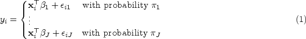
Let ${\mathbf{x}}_i^{\mathrm{\top }}=(x_{i,1},\dots ,x_{i,p})$ be the vector of $p$ explanatory variables for the $i$ th subject in a random sample of size $n$ . Let $\mathbf{y}=(y_1,\dots ,y_n)$ and $\mathbf{X}=({\mathbf{x}}_1^{\mathrm{\top }},\dots ,{\mathbf{x}}_n^{\mathrm{\top }}{)}^{\mathrm{\top }}$ denote the response vector and the full column rank ( $n\times p$ ) design matrix with $\text{rank}(\mathbf{X})=p<n$ . The regression model $y_i={\mathbf{x}}_i^{\mathrm{\top }}\beta +{ϵ}_i$ for $i=1,\dots ,n$ is one of the most common statistical methods to study the relationship between response variable and the set of the explanatory variables.

The mixture of regression models is a generalization of the regression model when the underlying population comprises of heterogeneous subpopulations. The mixture of regression models is defined by

$$\begin{array}{r}{y}_i=\{\begin{array}{lc}{\mathbf{x}}_i^{\mathrm{\top }}{\beta }_1+{ϵ}_{i1}& \text{with probability }{\pi }_1\\ ⋮\\ {\mathbf{x}}_i^{\mathrm{\top }}{\beta }_J+{ϵ}_{iJ}& \text{with probability }{\pi }_J\end{array}\end{array}$$

(1)

where ${\beta }_j=({\beta }_{j,1},\dots ,{\beta }_{J,p})$ represents the coefficients of $p$ predictors in the $j$ th component regression for $j=1,\dots ,J$ and $\pi =({\pi }_1,\dots ,{\pi }_J)$ denotes the vector of mixing proportions with $\sum _{j=1}^M{\pi }_j=1$ and $0<{\pi }_j<1$ . Also ${ϵ}_{ij}$ are independent normal random errors from each component of the mixture; that is ${ϵ}_{ij}\stackrel{iid}{\sim }N(0,{\sigma }_j^2)$ . Although we assume that the number of components $J$ in the mixture model (1) is known throughout the paper, the component memberships of the observations are unknown and should be estimated in an unsupervised approach. Let $\beta =({\beta }_1,\dots ,{\beta }_J)$ . Let ${\theta }_j=({\beta }_j,{\sigma }_j^2)$ denote the parameters of the $j$ th component. Thus, we represent the vector of all unknown parameters of the mixture (1) with $\mathbf{\Psi }=(\pi ,{\theta }_1,\dots ,{\theta }_J)$ .

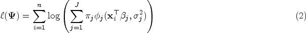
From regression model (1), the log-likelihood function of $\mathbf{\Psi }$ can be written as

$$\ell (\mathbf{\Psi })=\sum _{i=1}^n\log (\sum _{j=1}^J{\pi }_j{\varphi }_j({\mathbf{x}}_i^{\mathrm{\top }}{\beta }_j,{\sigma }_j^2))$$

(2)

where ${\varphi }_j({\mathbf{x}}_i^{\mathrm{\top }}{\beta }_j,{\sigma }_j^2)$ represents the pdf of the univariate normal distribution with mean ${\mathbf{x}}_i^{\mathrm{\top }}{\beta }_j$ and variance ${\sigma }_j^2$ . We need to maximize (2) in order to obtain the ML estimate of $\mathbf{\Psi }$ . The gradient of (2) is not tractable with respect to component parameters ${\theta }_j,j=1,\dots ,J$ . We view $(\mathbf{X},\mathbf{y})$ as incomplete data and apply the EM algorithm of Dempster et al. ¹⁰ using a complete data to find ${\hat{\mathbf{\Psi }}}_{ML}$ . For each subject $({\mathbf{x}}_i,y_i)$ , we introduce latent variables ${\mathbf{Z}}_i=(Z_{i1},\dots ,Z_{iJ})$ for $i=1,\dots ,n$ as

$$\begin{array}{r}{Z}_{ij}=\{\begin{array}{lc}1& \text{if the }i\text{th subject comes from the }j\text{th component,}\\ 0& o.w.,\end{array}\end{array}$$

where ${\mathbf{Z}}_i\stackrel{iid}{\sim }\text{Multi}(1,{\pi }_1,\dots ,{\pi }_M)$ . From the marginal distribution of latent variables, the conditional distribution of ${\mathbf{Z}}_i|y_i$ is given by

$$f({\mathbf{z}}_i|y_i)=\prod _{j=1}^J{\left\{\frac{{\pi }_j{\varphi }_j({\mathbf{x}}_i^{\mathrm{\top }}{\beta }_j,{\sigma }_j^2)}{\sum _{j=1}^J{\pi }_j{\varphi }_j({\mathbf{x}}_i^{\mathrm{\top }}{\beta }_j,{\sigma }_j^2)}\right\}}^{z_{ij}}$$

(3)

From the above, it is easily seen that ${\mathbf{Z}}_i|y_i\stackrel{iid}{\sim }\text{Multi}(1,{\tau }_{i1}(\mathbf{\Psi }),\dots ,{\tau }_{iJ}(\mathbf{\Psi }))$ where

$${\tau }_{ij}(\mathbf{\Psi })=\frac{{\pi }_j{\varphi }_j({\mathbf{x}}_i^{\mathrm{\top }}{\beta }_j,{\sigma }_j^2)}{\sum _{j=1}^J{\pi }_j{\varphi }_j({\mathbf{x}}_i^{\mathrm{\top }}{\beta }_j,{\sigma }_j^2)}$$

(4)

Let $(\mathbf{X},\mathbf{y},\mathbf{Z})$ denote the complete data. Thus, the complete log-likelihood function of $\mathbf{\Psi }$ is given by

$${\ell }_c(\mathbf{\Psi })=\sum _{i=1}^n\sum _{j=1}^J{z}_{ij}\log ({\pi }_j)+\sum _{i=1}^n\sum _{j=1}^J{z}_{ij}\log \{{\varphi }_j({\mathbf{x}}_i^{\mathrm{\top }}{\beta }_j,{\sigma }_j^2)\}$$

(5)

2.1. ML estimation method

The EM algorithm is a standard method to find the ML estimates of the mixture model parameters. The EM algorithm employs the latent variables on top of the observed data and decomposes the estimation procedure into an iterative expectation (E) and maximization (M) steps. As an iterative method, EM algorithm begins with an initial value. Let ${\mathbf{\Psi }}^{(0)}=({\pi }^{(0)},{\theta }_1^{(0)},\dots ,{\theta }_J^{(0)})$ and ${\mathbf{\Psi }}^{(r)}$ denote the initial vector and the estimate in the $r$ th iteration of the EM algorithm, respectively.

On the $(r+1)$ th iteration, we require to compute the conditional expectation of (5) in the E-step. The $Q(\mathbf{\Psi },{\mathbf{\Psi }}^{(r)})$ replaces the latent variables by their conditional expectations as

$$\mathbf{Q}(\mathbf{\Psi },{\mathbf{\Psi }}^{(r)})={\mathbf{Q}}_1(\pi ,{\mathbf{\Psi }}^{(r)})+{\mathbf{Q}}_2(\theta ,{\mathbf{\Psi }}^{(r)})$$

where

$${\mathbf{Q}}_1(\pi ,{\mathbf{\Psi }}^{(r)})=\sum _{i=1}^n\sum _{j=1}^J{\tau }_{ij}({\mathbf{\Psi }}^{(r)})\log ({\pi }_j)$$

(6)

and

$${\mathbf{Q}}_2(\theta ,{\mathbf{\Psi }}^{(r)})=\sum _{i=1}^n\sum _{j=1}^J{\tau }_{ij}({\mathbf{\Psi }}^{(r)})\log \{{\varphi }_j({\mathbf{x}}_i^{\mathrm{\top }}{\beta }_j,{\sigma }_j^2)\}$$

(7)

where ${\tau }_{ij}({\mathbf{\Psi }}^{(r)})$ is obtained by (4). In the M-step, we maximize $\mathbf{Q}(\mathbf{\Psi },{\mathbf{\Psi }}^{(r)})$ with respect to $\pi$ and $\theta$ to update ${\mathbf{\Psi }}^{(r+1)}$ . One can update ${\pi }^{(r+1)}$ by maximizing ${\mathbf{Q}}_1(\pi ,{\mathbf{\Psi }}^{(r)})$ subject to $\sum _{j=1}^J{\pi }_j=1$ as follows

$${\hat{\pi }}_j^{(r+1)}=\sum _{i=1}^n{\tau }_{ij}({\mathbf{\Psi }}^{(r)})/n;j=1,\dots ,J-1$$

(8)

The maximization of ${\mathbf{Q}}_2(\theta ,{\mathbf{\Psi }}^{(r)})$ can be reformulated by the weighted least squares (WLS) method as

$${\hat{\beta }}_j^{(r+1)}=\underset{{\beta }_j}{\arg min}(\mathbf{y}-\mathbf{X}\beta {)}^{\mathrm{\top }}{\mathbf{W}}_j(\mathbf{y}-\mathbf{X}\beta )/n$$

(9)

where ${\mathbf{W}}_j$ is $n\times n$ diagonal matrix with diagonal elements $({\tau }_{ij}({\mathbf{\Psi }}^{(r)}),\dots ,{\tau }_{nj}({\mathbf{\Psi }}^{(r)}))$ for all $j=1,\dots ,J$ . One can easily update ${\hat{\beta }}_j^{(r+1)}$ as the solution to (9) by

$$\begin{array}{r}{\hat{\beta }}_j^{(r+1)}={\left({\mathbf{X}}^{\mathrm{\top }}{\mathbf{W}}_j\mathbf{X}\right)}^{-1}{\mathbf{X}}^{\mathrm{\top }}{\mathbf{W}}_j\mathbf{y},j=1,\dots ,J\end{array}$$

(10)

From (9) and following, ¹⁴ we then update ${\hat{\sigma }}_j^{2(r+1)}$ as follows

$${\hat{\sigma }}_j^{2(r+1)}=\frac{(\mathbf{y}-\mathbf{X}{\hat{\beta }}_j^{(r+1)}{)}^{\mathrm{\top }}{\mathbf{W}}_j^{(r)}(\mathbf{y}-\mathbf{X}{\hat{\beta }}_j^{(r+1)})}{\sum _{i=1}^n{\tau }_{ij}({\mathbf{\Psi }}^{(r)})},j=1,\dots ,J$$

(11)

To find ${\hat{\mathbf{\Psi }}}_{ML}$ , we iteratively alternate the E- and M- steps of the EM algorithm until the stopping criterion $|\ell ({\mathbf{\Psi }}^{(r+1)})-\ell ({\mathbf{\Psi }}^{(r)})|$ becomes negligible.

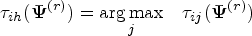
CEM Algorithm: In the above EM algorithm, we use information from all observations (as membership probabilities) in each iteration to estimate the parameters of the mixture model. Following Celeux and Govaert, ¹² we shall employ the classification version of EM algorithm (CEM) to estimate $\mathbf{\Psi }$ . The CEM algorithm incorporates a classification (C) step between E and M steps so that the component parameters of the mixture are updated in M-step using the classified complete data log-likelihood function.

The E-step here is identical to the E-step of the EM algorithm. In C-step, the observations are then assigned to $J$ mutually exclusive partitions corresponding to the $J$ components of mixture model (1). Let ${\mathbf{P}}^{(r+1)}=(P_1^{(r+1)},\dots ,P_J^{(r+1)})$ denote the partition in the $(r+1)$ th iteration. Each subject $({\mathbf{x}}_i,y_i)$ is assigned to partition $P_h^{(r+1)}$ when

$${\tau }_{ih}({\mathbf{\Psi }}^{(r)})=\underset{j}{\arg max}{\tau }_{ij}({\mathbf{\Psi }}^{(r)})$$

Note when the maximum weight is not unique, the tie is broken at random. Also the CEM algorithm is stopped and ${\mathbf{\Psi }}^{(r)}$ is returned when a partition becomes empty or has only one observation.

In the M-step, we maximize conditional expectation function using ${\mathbf{P}}^{(r+1)}$ . From (6), the mixing proportion is updated by

$${\hat{\pi }}_j^{(r+1)}=n_j/n;j=1,\dots ,J$$

(12)

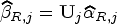
where $n_j$ is the number of observations allocated to partition $P_j^{(r+1)}$ . Applying the WLS to each partition $P_j^{(r+1)}$ , we can update the parameters of the $j$ th component ( $j=1,\dots ,J$ ) by

$$\begin{array}{rl}{\hat{\beta }}_j^{(r+1)}& ={\left({\mathbf{X}}_j^{\mathrm{\top }}{\mathbf{W}}_j{\mathbf{X}}_j\right)}^{-1}{\mathbf{X}}_j^{\mathrm{\top }}{\mathbf{W}}_j{\mathbf{y}}_j\end{array}$$

(13)

$$\begin{array}{rl}{\hat{\sigma }}_j^{2(r+1)}& =\frac{({\mathbf{y}}_j-{\mathbf{X}}_j{\hat{\beta }}_j^{(r+1)}{)}^{\mathrm{\top }}{\mathbf{W}}_j^{(r)}({\mathbf{y}}_j-{\mathbf{X}}_j{\hat{\beta }}_j^{(r+1)})}{\sum _{i=1}^n{\tau }_{ij}({\mathbf{\Psi }}^{(r)})}\end{array}$$

(14)

where ${\mathbf{X}}_j$ and ${\mathbf{y}}_j$ represent, respectively, $(n_j\times p)$ design matrix and vector of responses corresponding to $P_j^{(r+1)}$ . Also ${\mathbf{W}}_j^{(r)}$ is the diagonal weight matrix of size $n_j$ with entries $({\tau }_{ij}({\mathbf{\Psi }}^{(r)}),\dots ,{\tau }_{n_j,j}({\mathbf{\Psi }}^{(r)}))$ . Finally, we alternate repeatedly the E-, C- and M- steps until $|\ell ({\mathbf{\Psi }}^{(r+1)})-\ell ({\mathbf{\Psi }}^{(r)})|<ϵ$ .

SEM Algorithm: One can also apply the stochastic version of the EM algorithm ¹¹ to fit the mixture of regression models. The SEM algorithm implements a stochastic version of the C-step between E- and M-steps. Although the E- and M-steps are identical to the CEM algorithm, the SEM simulates the component membership of each observation using conditional distribution of the latent variable given incomplete data. On the $(r+1)$ th iteration, the S-step simulates a random allocation for each observation using one draw out of $J$ components as

$${\mathbf{Z}}_i^{*}=(Z_{i1}^{*},\dots ,Z_{iJ}^{*})\stackrel{iid}{\sim }\text{Multi}(1,{\tau }_{i1}({\mathbf{\Psi }}^{(r)}),\dots ,{\tau }_{iJ}({\mathbf{\Psi }}^{(r)}))(i=1,\dots ,n)$$

Then the $({\mathbf{x}}_i,y_i)$ is classified to partition $P_j^{(r+1)}$ if $Z_{ij}^{*}=1;i=1,\dots ,j=1,\dots ,J$ . Using the stochastic partitions, we update the mixture parameters from (12), (13) and (14) in M-step. From,^11,14 point-wise convergence in the SEM algorithm is not guaranteed. The algorithm resembles a Markov chain where at stationary state fluctuates around the ML estimate. Hence, we alternate the E-, S- and M-steps until either the criterion $|\ell ({\mathbf{\Psi }}^{(r+1)})-\ell ({\mathbf{\Psi }}^{(r)})|<ϵ$ satisfies or the chain reaches a prespecified maximum number of iterations that is fixed for all the algorithms for fair comparison.

2.2. Ridge estimation method

The ML method is a standard tool to estimate $\mathbf{\Psi }$ ; however, the ML estimates are dramatically influenced by multicollinearity where the covariates are linearly dependent. Ridge method ²⁷ is one of the most common methods to encounter with the challenges of the LS method. The ridge estimate for (1) can be obtained as a solution to the penalized log-likelihood function given by

$${\ell }^R(\mathbf{\Psi })=\ell (\mathbf{\Psi })-k{\beta }^{\mathrm{\top }}\beta /2$$

(15)

where $\ell (\mathbf{\Psi })$ comes from (2) and $k>0$ is the ridge parameter. In a similar vein to Subsection 2.1, for each observation $({\mathbf{x}}_i,y_i),i=1,\dots ,n$ , we first introduce $J$ dimensional latent vector ${\mathbf{Z}}_i=(Z_{i1},\dots ,Z_{iJ})$ . We then develop an EM algorithm to maximize the complete ridge log-likelihood function and obtain ${\hat{\mathbf{\Psi }}}_R$ .

The E-step of the ridge EM algorithm is identical to the E-step of Subsection 2.1. In the M-step, the mixing proportion are updated from (8). To update the coefficients of the component regressions, we require to maximize ${\mathbf{Q}}_2(\theta ,{\mathbf{\Psi }}^{(r)})$ subject to the ridge penalty within each component as

$${\mathbf{Q}}_2^R(\theta ,{\mathbf{\Psi }}^{(r)})={\mathbf{Q}}_2(\theta ,{\mathbf{\Psi }}^{(r)})-k_j{\beta }_j^{\mathrm{\top }}{\beta }_j/2$$

where ${\mathbf{Q}}_2(\theta ,{\mathbf{\Psi }}^{(r)})$ is from (7) and $k_j$ is the ridge parameter in the $j$ th component. Like ML method, one can re-write the maximization of ${\mathbf{Q}}_2^R(\theta ,{\mathbf{\Psi }}^{(r)})$ as a WLS subject to the ridge penalty by

$${\hat{\beta }}_{R,j}^{(r+1)}=\underset{{\beta }_j}{\arg min}(\mathbf{y}-\mathbf{X}{\beta }_j{)}^{\mathrm{\top }}{\mathbf{W}}_j(\mathbf{y}-\mathbf{X}{\beta }_j)+k_j{\beta }_j^{\mathrm{\top }}{\beta }_j/2$$

(16)

where ${\mathbf{W}}_j$ is $n\times n$ diagonal matrix with elements $({\tau }_{ij}({\mathbf{\Psi }}^{(r)}),\dots ,{\tau }_{nj}({\mathbf{\Psi }}^{(r)}))$ obtained from (4). Applying (16), ${\hat{\beta }}_j^{(r+1)};j=1,\dots ,J$ is updated by

$${\hat{\beta }}_{R,j}^{(r+1)}={({\mathbf{X}}^{\mathrm{\top }}{\mathbf{W}}_j\mathbf{X}+k_j\mathbb{I})}^{-1}{\mathbf{X}}^{\mathrm{\top }}{\mathbf{W}}_j\mathbf{y}$$

(17)

Lemma 1

Under the assumptions of mixture of regression models (1), suppose ${\lambda }_{1j},\dots ,{\lambda }_{pj}$ and $u_{1j},\dots ,u_{pj}$ are the eigenvalues and orthonormal eigenvectors of ${\mathbf{X}}^{\mathrm{\top }}{\mathbf{W}}_j\mathbf{X}$ where ${\mathbf{W}}_j$ is $n\times n$ diagonal matrix with entries $({\tau }_{ij}({\mathbf{\Psi }}^{(r)}),\dots ,{\tau }_{nj}({\mathbf{\Psi }}^{(r)}))$ under ridge EM algorithm. Let ${\mathbf{\Lambda }}_j=\text{diag}({\lambda }_{1j},\dots ,{\lambda }_{pj})$ and ${\mathbf{U}}_j=[u_{1j},\dots ,u_{pj}]$ . Then the canonical weighted ridge estimator in each component regression is given by

$${\hat{\alpha }}_{R,j}={({\mathbf{\Lambda }}_j+k_j\mathbb{I})}^{-1}{\mathbf{\Lambda }}_j^{1/2}{\mathbf{V}}_1^{\mathrm{\top }}{\mathbf{W}}_j^{1/2}\mathbf{y}$$

and

$${\hat{\beta }}_{R,j}={\mathbf{U}}_j{\hat{\alpha }}_{R,j}$$

with ${\mathbf{V}}_1=[v_{1j},\dots ,v_{pj}]$ where $v_{1j},\dots ,v_{pj}$ are the orthonormal eigenvectors of ${\mathbf{W}}_j^{1/2}\mathbf{X}{\mathbf{X}}^{\mathrm{\top }}{\mathbf{W}}_j^{1/2}$ .

From (16), the variance term can be updated by

$${\hat{\sigma }}_{R,j}^{2(r+1)}=\frac{(\mathbf{y}-\mathbf{X}{\hat{\beta }}_{R,j}^{(r+1)}{)}^{\mathrm{\top }}{\mathbf{W}}_j^{(r)}(\mathbf{y}-\mathbf{X}{\hat{\beta }}_{R,j}^{(r+1)})}{\sum _{i=1}^n{\tau }_{ij}({\mathbf{\Psi }}^{(r)})}$$

(18)

There are various methods available in the literature for the estimation of $k_j$ . Following Hoerl et al. ²⁸ , Liu ⁶ , we estimate the parameter by ${\hat{k}}_j=p{\hat{\sigma }}_{ML,j}^2/{\hat{\beta }}_{ML,j}^{\mathrm{\top }}{\hat{\beta }}_{ML,j}$ where ${\hat{\sigma }}_{ML,j}^2$ and ${\hat{\beta }}_{ML,j}$ are calculated from (11) and (10), respectively. The E- and M-steps are repeatedly computed until $|{\ell }^R({\mathbf{\Psi }}^{(r+1)})-{\ell }^R({\mathbf{\Psi }}^{(r)})|<ϵ$ .

Ridge CEM Algorithm: One can also apply the CEM algorithm to find ${\hat{\mathbf{\Psi }}}_R$ . Similar to the CEM algorithm in Subsection 2.1, we require to accommodate a C-step between E- and M-steps in the ridge EM algorithm. Here the E-step remains the same as before. Similar to the C-step of ML method, we classify the observations to partitions ${\mathbf{P}}^{(r+1)}=(P_1^{(r+1)},\dots ,P_J^{(r+1)})$ based on the maximum probability of memberships; that is

$$P_j^{(r+1)}=\{({\mathbf{x}}_i,y_i);{\tau }_{ij}({\mathbf{\Psi }}^{(r)})=\underset{h}{\arg max}{\tau }_{ih}({\mathbf{\Psi }}^{(r)})\},\mathrm{\forall }j=1,\dots ,J$$

Based on ${\mathbf{P}}^{(r+1)}$ , we use (12) to update the mixing proportions of the mixture. The ridge parameters are estimated similar to the ridge EM algorithm. We apply (16) to each partition $P_j^{(r+1)}$ and update the coefficients and variance term of each component regression by

$$\begin{array}{rl}{\hat{\beta }}_{R,j}^{(r+1)}& ={({\mathbf{X}}_j^{\mathrm{\top }}{\mathbf{W}}_j{\mathbf{X}}_j+k_j\mathbb{I})}^{-1}{\mathbf{X}}_j^{\mathrm{\top }}{\mathbf{W}}_j{\mathbf{y}}_j\end{array}$$

(19)

$$\begin{array}{rl}{\hat{\sigma }}_{R,j}^{2(r+1)}& =\frac{({\mathbf{y}}_j-{\mathbf{X}}_j{\hat{\beta }}_{R,j}^{(r+1)}{)}^{\mathrm{\top }}{\mathbf{W}}_j^{(r)}({\mathbf{y}}_j-{\mathbf{X}}_j{\hat{\beta }}_{R,j}^{(r+1)})}{\sum _{i=1}^n{\tau }_{ij}({\mathbf{\Psi }}^{(r)})}\end{array}$$

(20)

where ${\mathbf{X}}_j$ is $(n_j\times p)$ design matrix and ${\mathbf{y}}_j$ is vector of responses from observations classified to $P_j^{(r+1)}$ . ${\mathbf{W}}_j^{(r)}$ is the diagonal weight matrix with entries $({\tau }_{ij}({\mathbf{\Psi }}^{(r)}),\dots ,{\tau }_{n_j,j}({\mathbf{\Psi }}^{(r)}))$ from (4). Finally, the E-, C-, and M- steps under ridge estimation procedure are alternated until convergence criterion is satisfied.

Ridge SEM Algorithm: Ridge estimation method can be implemented via the SEM algorithm. Like SEM of ML method, the S-step determines stochastically the component membership of observations under ridge method by ${\mathbf{Z}}_i^{*}=(Z_{i1}^{*},\dots ,Z_{iJ}^{*})\stackrel{iid}{\sim }\text{Multi}(1,{\tau }_{i1}({\mathbf{\Psi }}^{(r)}),\dots ,{\tau }_{iJ}({\mathbf{\Psi }}^{(r)}));i=1,\dots ,n$ and updates ${\mathbf{P}}^{(r+1)}=(P_1^{(r+1)},\dots ,P_J^{(r+1)})$ such that $P_j^{(r+1)}=\{({\mathbf{x}}_i,y_i);Z_{ij}^{*}=1\};\mathrm{\forall }j=1,\dots ,J$ . Based on this stochastic partition of S-step, we update the mixture parameters by (12), (19) and (20).

Lemma 2

Under the assumptions of mixture of regression models (1)(with component regression models ${\mathbf{y}}_j={\mathbf{X}}_j{\beta }_j+ϵ$ based on $n_j$ observations and $\text{rank}({\mathbf{X}}_j)=p$ ), suppose ${\lambda }_{1j},\dots ,{\lambda }_{pj}$ and $u_{1j},\dots ,u_{pj}$ are the eigenvalues and orthonormal eigenvectors of ${\mathbf{X}}_j^{\mathrm{\top }}{\mathbf{W}}_j{\mathbf{X}}_j$ where ${\mathbf{W}}_j$ is a $n_j\times n_j$ diagonal matrix with entries $({\tau }_{ij}({\mathbf{\Psi }}^{(r)}),\dots ,{\tau }_{nj}({\mathbf{\Psi }}^{(r)}))$ under the ridge CEM or ridge SEM algorithm. Let ${\mathbf{\Lambda }}_j=\text{diag}({\lambda }_{1j},\dots ,{\lambda }_{pj})$ and ${\mathbf{U}}_j=[u_{1j},\dots ,u_{pj}]$ . Then the canonical weighted ridge estimator in each component regression is given by

$${\hat{\alpha }}_{R,j}={({\mathbf{\Lambda }}_j+k_j\mathbb{I})}^{-1}{\mathbf{\Lambda }}_j^{1/2}{\mathbf{V}}_1^{\mathrm{\top }}{\mathbf{W}}_j^{1/2}\mathbf{y}$$

and

$${\hat{\beta }}_{R,j}={\mathbf{U}}_j{\hat{\alpha }}_{R,j}$$

with ${\mathbf{V}}_1=[v_{1j},\dots ,v_{pj}]$ where $v_{1j},\dots ,v_{pj}$ are the orthonormal eigenvectors of ${\mathbf{W}}_j^{1/2}{\mathbf{X}}_j{\mathbf{X}}_j^{\mathrm{\top }}{\mathbf{W}}_j^{1/2}$ .

Finally, the E-, S-, and M-steps are iterated until the stopping rule is satisfied or the algorithm reaches a prespecified maximum number of iterations.

2.3. LT estimation method

When the design matrix is severely ill-conditioned, adding small values to the diagonal elements by the ridge estimator may be insufficient in addressing the issue. On the other hand, increasing the ridge parameter may result in a more considerable bias in the ridge estimation method. The LT shrinkage method for the multicollinearity in estimating the regression parameters was proposed in Liu. ⁶ Like the ridge method, the LT method optimizes the estimating equation subject to the LT penalty to control the multicollinearity. The LT penalty is given by

$$(-\frac{d}{k^{1/2}})\hat{\beta }=k^{1/2}\beta +{ϵ}^{\prime }$$

(21)

where $\hat{\beta }$ can be any estimator of coefficients and $d\in \mathbb{R}$ and $k>0$ are two parameters of the LT method. We develop the LT shrinkage method in estimating the unknown parameters of the mixture model (1). We shall find the LT estimate of $\mathbf{\Psi }$ by maximizing the log-likelihood function (2) subject to the LT penalty.

Similar to Section 2.1, the penalized log-likelihood function based on observed data is not tractable with respect to the component parameters. We develop the LT estimation procedure through an unsupervised approach and use the EM algorithm to estimate $\mathbf{\Psi }$ . We again require latent vectors ${\mathbf{Z}}_i=(Z_{i1},\dots ,Z_{iJ})$ to represent the component membership of the $i$ th observation $({\mathbf{x}}_i,y_i);i=1,\dots ,n$ . Let $(\mathbf{X},\mathbf{y},\mathbf{Z})$ denote the complete data. Then EM algorithm under the LT method proceeds as follows.

In $(r+1)$ th iteration, the E-step remains identical to the E-step of the ML method. The mixing proportions under the LT method are updated by (8). We require to maximize ${\mathbf{Q}}_2(\theta ,{\mathbf{\Psi }}^{(r)})$ from (7) under the LT penalty within each component to estimate the component parameters. The LT penalized log-likelihood function can be written as a WLS constrained on the LT penalty as

$$\begin{array}{rl}{\hat{\beta }}_{LT,j}^{(r+1)}& =\underset{{\beta }_j}{\arg min}(\mathbf{y}-\mathbf{X}{\beta }_j{)}^{\mathrm{\top }}{\mathbf{W}}_j(\mathbf{y}-\mathbf{X}{\beta }_j)\\ & +{[(-\frac{d_j}{k_j^{1/2}}){\hat{\beta }}_j-k_j^{1/2}{\beta }_j]}^{\mathrm{\top }}[(-\frac{d_j}{k_j^{1/2}}){\hat{\beta }}_j-k_j^{1/2}{\beta }_j]\end{array}$$

(22)

where ${\hat{\beta }}_j$ can be any estimate and ${\mathbf{W}}_j$ is a weight diagonal matrix with elements $({\tau }_{1j}({\mathbf{\Psi }}^{(r)}),\dots ,{\tau }_{nj}({\mathbf{\Psi }}^{(r)});j=1,\dots ,J$ . From (22), the coefficients and variance terms in each component regression are updated by

$$\begin{array}{rl}{\hat{\beta }}_{LT,j}^{(r+1)}& ={({\mathbf{X}}^{\mathrm{\top }}{\mathbf{W}}_j\mathbf{X}+k_j\mathbb{I})}^{-1}({\mathbf{X}}^{\mathrm{\top }}{\mathbf{W}}_j\mathbf{y}-d_j{\hat{\beta }}_j)\end{array}$$

(23)

$$\begin{array}{rl}{\hat{\sigma }}_{LT,j}^{2(r+1)}& =\frac{(\mathbf{y}-\mathbf{X}{\hat{\beta }}_{LT,j}^{(r+1)}{)}^{\mathrm{\top }}{\mathbf{W}}_j^{(r)}(\mathbf{y}-\mathbf{X}{\hat{\beta }}_{LT,j}^{(r+1)})}{\sum _{i=1}^n{\tau }_{ij}({\mathbf{\Psi }}^{(r)})}\end{array}$$

(24)

Equations (23) and (24) require the estimates of the LT parameters $(k_j,d_j)$ for each component regression. From Liu, ⁶ we can estimate $k_j$ in the $j$ th component by ${\hat{k}}_{LT,j}=({\lambda }_{1,j}-100{\lambda }_{p,j})/99$ where ${\lambda }_{1,j}$ and ${\lambda }_{p,j}$ are the maximum and the minimum eigenvalues of ${\mathbf{X}}^{\mathrm{\top }}{\mathbf{W}}_j\mathbf{X}$ on the $(r+1)$ the iteration of the EM algorithm.

Lemma 3

Under the assumptions of Lemma (1), the canonical LT estimator in the $j$ th component regression $j=1,\dots ,J$ under EM algorithm is given by

$${\hat{\alpha }}_{LT,j}={({\mathbf{\Lambda }}_j+k_j\mathbb{I})}^{-1}({\mathbf{\Lambda }}_j^{1/2}{\mathbf{V}}_1^{\mathrm{\top }}{\mathbf{W}}_j^{1/2}\mathbf{y}-d_j{\hat{\alpha }}_j)$$

and

$$\begin{array}{r}{\hat{\beta }}_{LT,j}={\mathbf{U}}_j{\hat{\alpha }}_{LT,j}\end{array}$$

where ${\hat{\alpha }}_j$ is the canonical estimate of ${\beta }_j$ and ${\mathbf{V}}_1=[v_{1j},\dots ,v_{pj}]$ with $v_{1j},\dots ,v_{pj}$ are the orthonormal eigenvectors of ${\mathbf{W}}_j^{1/2}\mathbf{X}{\mathbf{X}}^{\mathrm{\top }}{\mathbf{W}}_j^{1/2}$ .

Following Liu ⁶ and Lemma 3, the optimal $d_j$ can be obtained by the next lemma within each component of the mixture of regression models.

Lemma 4

Under the assumptions of Lemma 1 and for each $k_j>0$ , we have

• (i)

when ${\hat{\alpha }}_j={\hat{\alpha }}_{ML,j}$ , then

$$d_j=\sum _{m=1}^p(({\sigma }_j^2-k_j{\alpha }_{mj}^2)/({\lambda }_{mj}+k_j{)}^2)/\sum _{m=1}^p(({\lambda }_{mj}{\alpha }_{mj}^2+{\sigma }_j^2)/{\lambda }_{mj}({\lambda }_{mj}+k_j{)}^2)$$

(ii)

when ${\hat{\alpha }}_j={\hat{\alpha }}_{R,j}$ , then

$$d_j=\sum _{m=1}^p({\lambda }_{mj}({\sigma }_j^2-k_j{\alpha }_{mj}^2)/({\lambda }_{mj}+k_j{)}^3)/\sum _{m=1}^p({\lambda }_{mj}({\lambda }_{mj}{\alpha }_{mj}^2+{\sigma }_j^2)/({\lambda }_{mj}+k_j{)}^4)$$

minimizes the $\text{MSE}({\hat{\alpha }}_{LT,j})$ within each component (1) in the EM algorithm of the LT method.

Although Lemma 4 paves the path in estimating the optimal LT parameter $d_j$ within each component regression, the optimal value still depends on the unknown quantities including ${\sigma }_j$ , $k_j$ , ${\alpha }_j$ and ${\lambda }_{m,j}$ for $m=1,\dots ,p$ and $j=1,\dots ,J$ . From Lemma 4, we propose a practical approach where $d_j,j=1,\dots ,J$ can be updated in the $(r+1)$ th iteration of the EM algorithm by

$${\hat{d}}_j=\sum _{m=1}^p({\lambda }_{mj}({\hat{\sigma }}_{R,j}^2-{\hat{k}}_j{\hat{\alpha }}_{R,mj}^2)/({\lambda }_{mj}+{\hat{k}}_j{)}^3)/\sum _{m=1}^p({\lambda }_{mj}({\lambda }_{mj}{\hat{\alpha }}_{R,mj}^2+{\hat{\sigma }}_{R,j}^4)/{\lambda }_{mj}({\lambda }_{mj}+{\hat{k}}_j{)}^2)$$

(25)

where ${\hat{k}}_j={\hat{k}}_{LT,j}$ , ${\hat{\alpha }}_{R,j}=({\hat{\alpha }}_{R,1j},\dots ,{\hat{\alpha }}_{R,pj})$ is given by Lemma 1 and $({\lambda }_{1j},\dots ,{\lambda }_{pj})$ are eigenvalues of ${\mathbf{X}}_j^{\mathrm{\top }}{\mathbf{W}}_j{\mathbf{X}}_j$ with ${\hat{\sigma }}_{R,j}^2$ from (18). The E- and M-steps are alternated until the stopping criterion is satisfied. As the parameters $k_j$ and $d_j$ are updated in each iteration of the EM algorithm, the proposed LT method is henceforth called the iterative LT i.e. Liu_ITE.

Unlike the iterative LT method, one can follow Hoerl et al. ²⁸ to estimate the LT parameters based on ridge estimates ${\hat{\sigma }}_{R,j}$ and ${\hat{\beta }}_{R,j}$ . In other words, the mixture parameter $\mathbf{\Psi }$ and $d_j$ are still iteratively updated in the EM algorithm; however, $k_j,j=1\dots ,J$ parameters are estimated only once throughout the EM algorithm using the ridge estimates. Here, we estimate the parameters by ${\hat{k}}_{LT,j}=p{\hat{\sigma }}_{R,j}/{\hat{\beta }}_{R,j}^{\mathrm{\top }}{\hat{\beta }}_{R,j}$ . This LT estimation method is henceforth called HKP LT i.e. Liu_HKP.

LT CEM algorithm: Like previous subsections, the CEM algorithm partitions the observations in the C-step and then update the parameters within each partition. In the $(r+1)$ th iteration of the CEM algorithm, the E-step remains the same as before. The C-step classifies the observations into partition ${\mathbf{P}}^{(r+1)}=(P_1^{(r+1)},\dots ,P_J^{(r+1)})$ where $P_j^{(r+1)}=\{({\mathbf{x}}_i,y_i);{\tau }_{ij}({\mathbf{\Psi }}^{(r)})=\underset{h}{\arg max}{\tau }_{ih}({\mathbf{\Psi }}^{(r)})\}$ with $({\tau }_{i1}({\mathbf{\Psi }}^{(r)}),\dots ,{\tau }_{iJ}({\mathbf{\Psi }}^{(r)}))$ are obtained from (4). Using ${\mathbf{P}}^{(r+1)}$ , we update the mixing proportions from (12). We then require to estimate the LT parameters $(k_j,d_j)$ in each iteration of the CEM algorithm. Similar to LT EM algorithm, we propose ${\hat{k}}_{LT,j}=({\lambda }_{1,j}-100{\lambda }_{p,j})/99$ where ${\lambda }_{1,j}$ and ${\lambda }_{p,j}$ are the maximum and the minimum eigenvalues of ${\mathbf{X}}_j^{\mathrm{\top }}{\mathbf{W}}_j{\mathbf{X}}_j$ .

Lemma 5

Under the assumptions of Lemma (1), the canonical LT estimator in the $j$ th component regression $j=1,\dots ,J$ under the CEM algorithm is given by

$${\hat{\alpha }}_{LT,j}={({\mathbf{\Lambda }}_j+k_j)}^{-1}({\mathbf{\Lambda }}_j^{1/2}{\mathbf{V}}_1^{\mathrm{\top }}{\mathbf{W}}_j^{1/2}\mathbf{y}-d_j{\hat{\alpha }}_j)$$

and

$${\hat{\beta }}_{LT,j}={\mathbf{U}}_j{\hat{\alpha }}_{LT,j}$$

where ${\hat{\alpha }}_j$ is the canonical estimate of ${\beta }_j$ and ${\mathbf{V}}_1=[v_{1j},\dots ,v_{pj}]$ with $v_{1j},\dots ,v_{pj}$ are the orthonormal eigenvectors of ${\mathbf{W}}_j^{1/2}{\mathbf{X}}_j{\mathbf{X}}_j^{\mathrm{\top }}{\mathbf{W}}_j^{1/2}$ .

From Lemmas 4 and 5 , one can estimate parameter $d_j$ based on partition $P_j^{(r+1)}$ from (25) where $({\lambda }_{1j},\dots ,{\lambda }_{pj})$ are eigenvalues of ${\mathbf{X}}_j^{\mathrm{\top }}{\mathbf{W}}_j{\mathbf{X}}_j$ and estimate ${\hat{\sigma }}_{R,j}^2$ from equation (20). To estimate the regression parameters, we implement a WLS based on the LT penalty as

$${\hat{\beta }}_{LT,j}^{(r+1)}=\underset{{\beta }_j}{\arg min}({\mathbf{y}}_j-{\mathbf{X}}_j{\beta }_j{)}^{\mathrm{\top }}{\mathbf{W}}_j({\mathbf{y}}_j-{\mathbf{X}}_j{\beta }_j)+{[(-\frac{{\hat{d}}_j}{{\hat{k}}_{LT,j}^{1/2}}){\hat{\beta }}_j-{\hat{k}}_{LT,j}^{1/2}{\beta }_j]}^{\mathrm{\top }}[(-\frac{{\hat{d}}_j}{{\hat{k}}_{LT,j}^{1/2}}){\hat{\beta }}_j-{\hat{k}}_{LT,j}^{1/2}{\beta }_j]$$

(26)

where ${\mathbf{y}}_j$ and ${\mathbf{X}}_j$ are response vector and design matrix under $P_j^{(r+1)}$ and ${\hat{\beta }}_j$ can be any estimate for ${\beta }_j$ . Also, ${\mathbf{W}}_j$ is a weight diagonal matrix with entries $({\tau }_{1j}({\mathbf{\Psi }}^{(r)}),\dots ,{\tau }_{n_j,j}({\mathbf{\Psi }}^{(r)}));j=1,\dots ,J$ . One can easily find the solution to equation (22) and update the regression parameters by

$$\begin{array}{rl}{\hat{\beta }}_{LT,j}^{(r+1)}& ={({\mathbf{X}}_j^{\mathrm{\top }}{\mathbf{W}}_j{\mathbf{X}}_j+{\hat{k}}_{LT,j}\mathbb{I})}^{-1}({\mathbf{X}}_j^{\mathrm{\top }}{\mathbf{W}}_j{\mathbf{y}}_j-{\hat{d}}_j{\hat{\beta }}_j)\end{array}$$

(27)

$$\begin{array}{rl}{\hat{\sigma }}_{LT,j}^{2(r+1)}& =\frac{({\mathbf{y}}_j-{\mathbf{X}}_j{\hat{\beta }}_{LT,j}^{(r+1)}{)}^{\mathrm{\top }}{\mathbf{W}}_j^{(r)}({\mathbf{y}}_j-{\mathbf{X}}_j{\hat{\beta }}_{LT,j}^{(r+1)})}{\sum _{i=1}^n{\tau }_{ij}({\mathbf{\Psi }}^{(r)})}\end{array}$$

(28)

The E-, C-, and M-steps are repeatedly computed until the convergence criterion is satisfied.

Unlike the iterative LT CEM algorithm, one may estimate the parameters of the mixture model via the HKP LT CEM algorithm where the LT parameters $(k_j,d_j),j=1,\dots ,J$ are updated once throughout the algorithm. From Hoerl et al., ²⁸ Liu, ⁶ we propose to estimate ${\hat{k}}_{LT,j}=p{\hat{\sigma }}_{R,j}/{\hat{\beta }}_{R,j}^{\mathrm{\top }}{\hat{\beta }}_{R,j}$ and ${\hat{d}}_j$ from equation (25) where ${\hat{\beta }}_{R,j}$ and ${\hat{\sigma }}_{R,j}$ come from equations (19) and (20), respectively.

LT SEM algorithm: Similar to the SEM algorithms, the S-step partitions the observations stochastically from $\text{Multi}(1,{\tau }_{i1}({\mathbf{\Psi }}^{(r)}),\dots ,{\tau }_{iJ}({\mathbf{\Psi }}^{(r)}))$ for $i=1,\dots ,n$ . Once the partition is established, the rest of the LT SEM algorithms are implemented similarly to the LT CEM algorithms.

3. Simulation studies

In this section, we examine the performance of the ML, Ridge, and LT methods when the underlying population is a mixture of linear regression models with multicollinearity problem. We present two simulations enabling us to study the effect of the sample size, multicollinearity levels, and the number of components of mixture models on the estimation and prediction of the proposed methods.

This paper investigates, for the first time in the literature, the Ridge and LT shrinkage methods for heterogeneous populations using a mixture of regression models. Hence, the main goal of the numerical studies is to compare the estimation performance of the biased shrinkage methods with the commonly used benchmark ML method in the presence of multicollinearity. Although the initial values play an essential role in iterative methods like the EM algorithm, in these simulations as comparative numerical studies, we have $(J\times p)$ matrix of coefficients, mixing proportions and variance terms to deal with the parameters of $J$ component regressions each with $p$ covariates. For these reasons, in all the numerical studies, we chose the initial values fixed, close to the true values of the parameters and the same for all the EM, CEM, and SEM approaches under ML, Ridge, and LT estimation methods for a fair comparison. Also, we used $|\ell ({\mathrm{\Psi }}^{(t+1)})-\ell ({\mathrm{\Psi }}^{(t)})|<{10}^{-5}$ as the stopping rule for all the estimation methods. We set the maximum number of iterations to be 2000 for all the EM, CEM, and SEM approaches under the ML, Ridge, and LT methods. We used a single start for all the numerical studies. If the EM algorithms, for any reason, did not converge in 2000 iterations, the estimate in the last iteration was treated as the solution in the EM algorithm.

It is well-known that a FMM’s log-likelihood may appear multimodal; hence, the EM algorithm may converge to local maxima. We designed the numerical studies in a comparative way to compare the estimation performance of the proposed shrinkage methods with those of the commonly used ML method. Since the log-likelihood of all the estimation methods is subject to this multimodality, we did not exclude the convergence to the local maxima for all the estimation methods for a fair comparison. Although the algorithms may converge to either local or global maxima, the overall estimation performance of the methods is evaluated. Therefore, the local maxima estimates in simulations indirectly affect the errors of the estimation algorithms.

In the first study, we simulate data from a population corresponding to a mixture of two regression models with four covariates $(x_1,\dots ,x_4)$ . Following Inan and Erdogan, ²⁹ we use $\rho$ to denote the correlation between covariates to simulate the multicollinearity in the mixture model. To do so, we first generate random numbers $\{w_{ij};i=1,\dots ,n;j=1,\dots ,5\}$ from the standard normal distribution. The covariates are then generated by

$$x_{ij}=(1-{\rho }^2{)}^{1/2}{w}_{ij}+\rho w_{i,5},j=1,\dots ,4$$

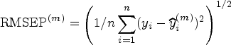
where the correlation matrix of $\mathbf{X}$ is given by $4\times 4$ whose diagonal entries are 1 and off-diagonal entries are equal to ${\rho }^2=cor(x_j,x_h);j,h=1,\dots ,4$ . Here, we set $\rho \in \{0.88,0.9,0.95,0.97,0.99\}$ to simulate the multicollinearity levels in the mixture of regression models. The responses are then generated from mixture model (1) whose true parameters are given by ${\mathbf{\Psi }}_0=({\pi }_0,{\beta }_{01},{\beta }_{02},{\sigma }_{01}^2,{\sigma }_{02}^2)$ with ${\pi }_0=0.7$ , ${\beta }_{01}=(1,3,4,5,6)$ , ${\beta }_{02}=(-1,-1,-2,-3,-5)$ and ${\sigma }_{01}^2={\sigma }_{02}^2=\{0.5,1,2\}$ . We measured the estimation performance of the ML, Ridge, and LT methods by root means square errors (RMSE) in estimating $(\pi ,\beta ,{\sigma }^2)$ and computed $\text{RMSE}(\hat{\beta })=[\frac{1}{M}(\hat{\beta }-{\beta }_0{)}^{\mathrm{\top }}(\hat{\beta }-{\beta }_0){]}^{1/2}$ , $\text{RMSE}(\hat{\pi })=\sqrt{(\hat{\pi }-{\pi }_0{)}^2}$ and $\text{RMSE}({\hat{\sigma }}^2)=[\frac{1}{M}({\hat{\sigma }}_m^2-{\sigma }_{0,m}^2{)}^{\mathrm{\top }}({\hat{\sigma }}_m^2-{\sigma }_{0,m}^2){]}^{1/2}$ , where $\hat{\beta }=({\hat{\beta }}_1,{\hat{\beta }}_2)$ , ${\hat{\sigma }}^2=({\hat{\sigma }}_1^2,{\hat{\sigma }}_2^2)$ , ${\hat{\beta }}_0=({\hat{\beta }}_{01},{\hat{\beta }}_{02})$ and ${\sigma }_0^2=({\sigma }_{01}^2,{\sigma }_{02}^2)$ and $M$ denotes teh number of free parameters. We also used the root mean squared errors of prediction (RMSEP) to evaluate the prediction performance of the methods. To do so, we first compute the RMSEP of the $m$ th replicate through $K$ -fold cross-validation by

$${\text{RMSEP}}^{(m)}={(1/n\sum _{i=1}^n(y_i-{\hat{y}}_i^{(m)}{)}^2)}^{1/2}$$

where ${\hat{y}}_i^{(m)}$ is the predicted response of the $i$ th observation in the $m$ th replicate.

We computed the estimation and prediction measures for the ML, Ridge, and LT methods as follows. We first generated a sample of size $n=\{60,100,200\}$ from the underlying mixture of regression models as described above. We selected the starting point of parameters as ${\pi }^{(0)}=0.5$ , ${\beta }_{01}^{(0)}=(-1,1,2,3,4)$ , ${\beta }_{02}^{(0)}=(1,1,0,-1,-3)$ and ${\sigma }^{2^{(0)}}=(1,2)$ . We then used the EM, CEM, and SEM algorithms to estimate the parameters of the mixture population via ML, Ridge, and LT methods. We applied the idea of $K=5$ cross-validation to assess the prediction performance of the methods. To this end, we divided the sample into $K$ folds of equal sizes. We used $K-1$ folds for training and the remaining fold for prediction. We repeated the procedure for all $k=1,\dots ,K$ to compute the ${\text{RMSEP}}^{(m)}$ . Eventually, we replicated the entire procedures $m=2000$ times and computed the median and 95% confidence interval (CI) for the SSE and RMSEP measures. The lower and upper bounds of the CI correspond to 2.5 and 97.5 percentiles of 2000 replications, respectively.

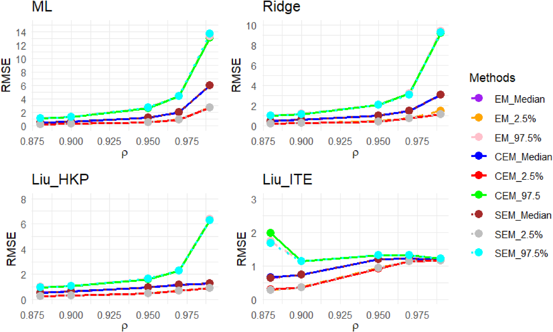
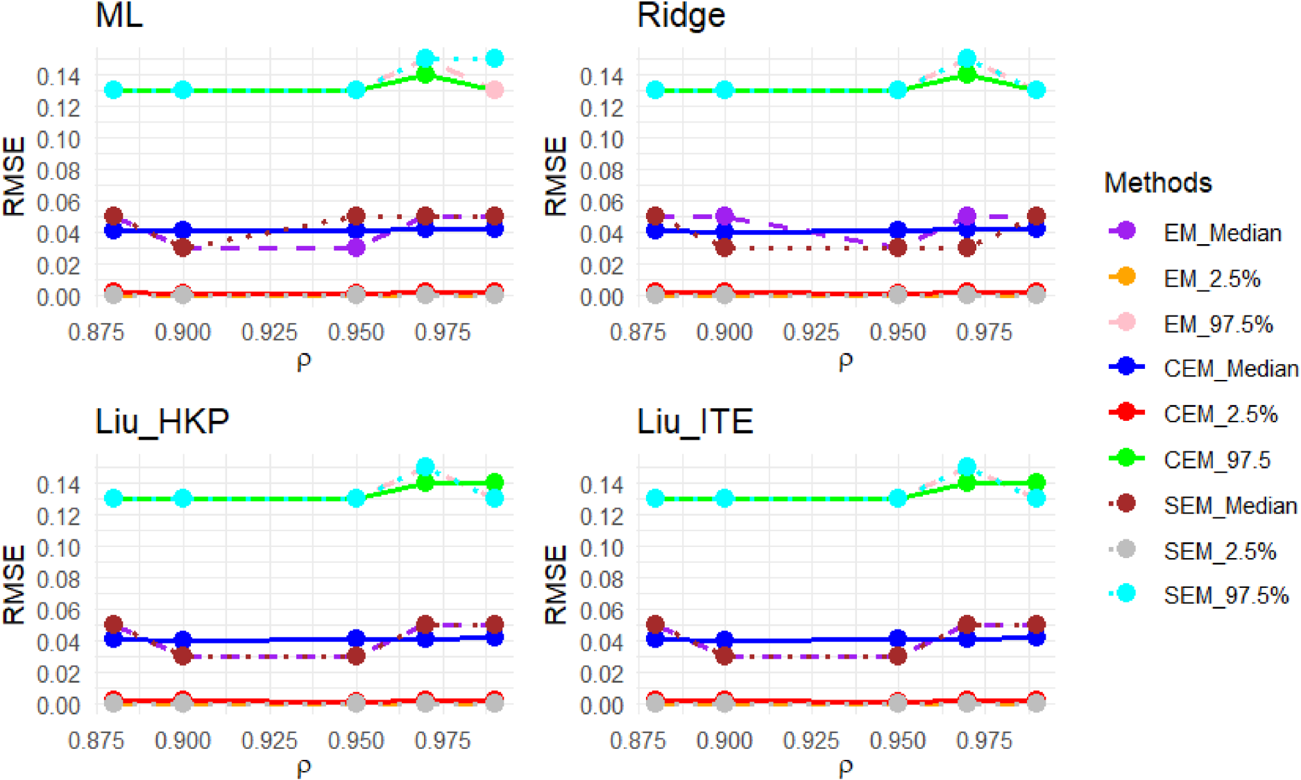
Due to sampling variability, the generated design matrix and response vector change from one replication to another in the simulation. Given this, Figure 55 (in the Appendix) reports the sampling distributions of the covariates and responses for a randomly selected sample with size $n=100$ and $\rho =0.95$ . Due to sampling variability, the sample correlation may change slightly from the nominal correlation. Accordingly, for the selected random sample, the sample variance inflation factors (VIFs) are almost around VIF = 45.70 in Figure 55. We show the results of the simulation study in estimating $(\pi ,\beta ,{\sigma }^2)$ in Figures 1 to 3 and 5 to 28 (in the Appendix). It is observed that the ML methods estimate slightly better the mixing proportion than the ridge and LT methods. This happens because the ridge and LT estimators are biased shrinkage methods where a slight bias is incorporated into the estimation to encounter the multicollinearity problem. We observe that the multicollinearity significantly impacts the ML estimates of the coefficients and results in extremely unreliable estimates for all EM, CEM, and SEM algorithms. Unlike ML estimates, a significant improvement is seen in the performance of the shrinkage methods in estimating the coefficients of the component regressions. The LT methods appear more reliable than their ridge counterparts in the multicollinearity. From a comparison between LT(ITR) and Liu_HKP, we see that Liu_HKP provides more reliable estimates for ${\sigma }^2$ . Among the Liu_HKP estimators, the CEM algorithm almost always outperforms its EM ad SEM counterparts. Tables 1 and 9 (in the Appendix) show the median and the length of 95% CI of the RMSEP for all the developed methods. The tables clearly show that the prediction performances of all the methods and EM algorithms are almost identical. This finding is consistent with Inan and Erdogan ²⁹ that multicollinearity seriously affects the estimation of the methods while prediction levels stay almost the same.

Figure 1.

The median, lower, and upper bounds of 95% CIs for $\text{RMSE}(\hat{\beta })$ of the estimators when the population is a mixture of two regression models with $n=60$ and ${\sigma }^2=0.5$ . RMSE: root means square error; CI: confidence interval.

Figure 2.

The median, lower, and upper bounds of 95% CIs for $\text{RMSE}(\hat{\pi })$ of the estimators when the population is a mixture of two regression models with $n=60$ and ${\sigma }^2=0.5$ . RMSE: root means square error; CI: confidence interval.

Figure 3.

The median, lower, and upper bounds of 95% CIs for $\text{RMSE}({\hat{\sigma }}^2)$ of the estimators when the population is a mixture of two regression models with $n=60$ and ${\sigma }^2=0.5$ . RMSE: root means square error; CI: confidence interval.

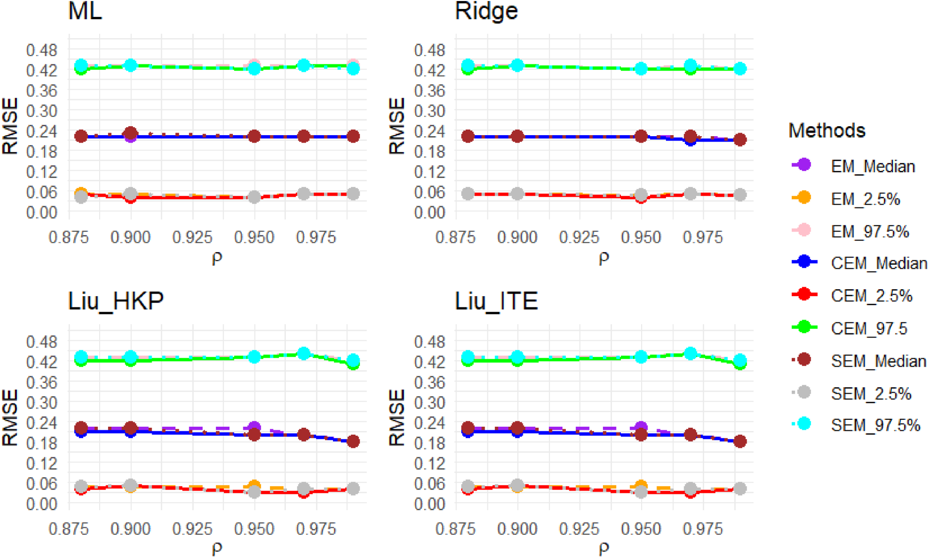
In the second simulation study, we evaluate the performance of the estimators when the underlying mixture model consists of three component regressions with two covariates. We set $\rho \in \{0.9,0.92,0.95,0.97,0.99\}$ to simulate the multicollinearity in the mixture. As described earlier, we generated the covariates and responses from the mixture model with parameters ${\pi }_0=({\pi }_{01},{\pi }_{02},{\pi }_{03})=(0.3,0.4,0.3)$ , ${\beta }_{01}=(1,3,4)$ , ${\beta }_{02}=(-1,-1,-2)$ , ${\beta }_{03}=(-3,1,-4)$ and ${\sigma }_0^2=(0.25,1,0.09)$ . For example, Figure 56 (in the Appendix) reports the sampling distributions of the covariates and responses for a randomly selected sample with size $n=100$ and $\rho =0.95$ . Accordingly, for the selected random sample, the sample VIF is almost around VIF = 10.25. Similar to the settings of the first simulation study, we replicated 2000 times all the estimation and prediction procedures under the EM, CEM, and SEM algorithms and computed the median and 95% CI for the SSEs and RMSEP for sizes $n=\{60,100,200\}$ . Here again, we set fixed and the same starting points for all the estimation methods. The employed starting points include ${\pi }^{(0)}=(0.3,0.4,0.3)$ , ${\beta }_{01}^{(0)}={\beta }_{01}-1$ , ${\beta }_{02}^{(0)}={\beta }_{02}-1$ , ${\beta }_{03}^{(0)}={\beta }_{03}-1$ and ${\sigma }^{2^{(0)}}={\sigma }^2+0.02$ . The estimation and prediction results are demonstrated in Figures 4 and 29 to 54 (in the Appendix) and Tables 13 to 21 (in the Appendix), respectively. Here, we also observe that the ML method slightly better estimates the mixing proportions; however, the ML methods result in unreliable estimates for the coefficients of component regressions. It is easy to see that shrinkage estimators do better in estimating the component regression parameters. In addition, the Liu_HKP almost always outperforms other methods and provides a more reliable estimate of the mixture of regression models. Therefore, the Liu_HKP method based on the CEM algorithm is recommended to fit the mixture of linear regression models in multicollinearity.

Figure 4.

The median, lower, and upper bounds of 95% CIs for $\text{RMSE}(\hat{\beta })$ of the estimators when the population is a mixture of three regression models with $n=60$ and ${\sigma }^2=0.5$ .

Although it is well known that the convergence of the SEM (SEM) algorithm (for all the estimation methods) is not guaranteed; the algorithm resembles a Markov chain that fluctuates around the ML estimate.^11,14 For this reason, for a fair comparison between all the estimation algorithms, we set the maximum number of iterations to be 2000 for all the EM, CEM, and SEM approaches. If the EM algorithms, for any reason, did not converge in 2000 iterations, the estimate in the last iteration was treated as the solution in the EM algorithm. It is also well known that the log-likelihood of the mixture model may appear multi-model, and the EM algorithm may trap in the local maxima. Although the algorithms in this manuscript may converge to either local or global maxima for all estimation methods, the overall estimation performance of the EM, CEM, and SEM of the ML, Ridge, and LT methods are evaluated in a comparative way using RMSE, which takes into account the squared distance of all the estimates from the true value of the parameters of the mixture model.

To this end, we designed the third simulation study to compare the convergence of the proposed shrinkage estimation algorithms with the commonly used ML counterparts using the same stopping rule. To do so, we used the tolerance levels $ϵ\in \{{10}^{-3},{10}^{-5}\}$ , while we kept the maximum number of iterations fixed for all methods and the same as 2000. We replicated 2000 times the entire data collection and the estimation in the same way as described above. We then computed the convergence rates of each estimation algorithm by the proportion of times the algorithm converged before reaching the maximum number of iterations. Table 22 (in the Appendix) demonstrates the convergence rates of the different estimation methods and EM algorithms under two different underlying mixtures of regression models with two and three components. From Table 22, we observe that the convergence rates of the Ridge and LT shrinkage methods outperform that of their ML counterpart using EM, CEM, and SEM algorithms in the presence of the multicollinearity. Moreover, this superiority is consistent across both tolerance levels, indicating the robustness of the shrinkage methods in achieving convergence. Additionally, the convergence rates highlight the stability and reliability of the proposed shrinkage estimation algorithms, suggesting their suitability for practical applications in scenarios characterized by multicollinearity.

4. Bone data analysis

As a bone metabolic disease, osteoporosis occurs when the bone mineral architecture of the body deteriorates. This deterioration results in skeletal fragility and a high risk of osteoporotic fractures in different body areas such as the hip and femur. Osteoporosis and its related diseases significantly impact the patient’s health and survival. For example, one out of every two patients with osteoporotic hip fractures can no longer live independently, and one out of three may die within one year after the medical complication of the broken bone.^2,30 The BMD of individuals improves until age 30 and then decreases as individuals age. The BMD score of an individual is compared with a BMD norm to determine the bone disorder status. The BMD norm is computed by the mean BMD scores of healthy adults aged 20–30. The bone status of an individual is diagnosed as osteoporosis when the BMD score is less than $-2.5$ SD from the BMD norm of the population.

The BMD scores are obtained via an expensive and time-consuming procedure. Despite this, the researchers have access to various easy-to-measure patients’ characteristics, such as age, weight, BMI, and test results from earlier surveys.^31,32 Regression models are among the most common methods to investigate the impact of a set of patients’ characteristics on the BMD responses. The impact of the characteristics may differ at different BMD levels. Hence, the inference on BMD measurements can be handled as a problem of the mixture of linear regression models.

The bone mineral data in this section were obtained from the National Health and Nutritional Examination Survey (NHANES III) administrated by the CDC on more than 33999 American adults between the years 1988–1994. The data set is publicly available on the website of the CDC from (https://wwwn.cdc.gov/nchs/nhanes/nhanes3/Default.aspx). One hundred eighty-two White women aged 50 and older participated in both bone examinations during the survey. Due to the substantial impact of osteoporosis on older women, these 182 women were considered our target population. From the second bone examination, we focused on femur BMD as the response variable. We also used two easily attainable physical characteristics as the explanatory variables of the regression. These physical characteristics include arm and bottom circumferences from the first examination. The association between the two explanatory variables is $\rho =0.81$ . Using the ML method based on the information of all individuals in the population, the BIC criterion suggests that a mixture of two regression models is the best fit with parameters ${\pi }_0=({\pi }_{01},{\pi }_{02})=(0.64,0.36)$ , ${\beta }_{01}=(0.004,0.006)$ , ${\beta }_{02}=(0.011,0.005)$ , and ${\sigma }_0^2=(0.0081,0.0144)$ . These parameters were then considered as the true parameters of the mixture population. Figure 57 reports the histograms of the explanatory variables and the responses for the two components. As an unsupervised learning, the true component membership of the observations was obtained as follows. The individuals whose BMD score is less than one standard deviation from the MD norm (the average of the BMD scores from the healthy adults between 20 and 30) were assigned to the first component (osteoporosis) and the others to the second component. We replicated 2000 times the ML, ridge, and LT methods under EM, CEM, and SEM algorithms in estimating the parameters of the bone mineral population based on sample sizes $n=\{60,100,200\}$ . Similar to Section 3, we selected the fixed and the same starting points for all estimation methods as ${\pi }^{(0)}=(0.7,0.3)$ , ${\beta }_{01}^{(0)}={\beta }_{01}+0.001$ , ${\beta }_{02}^{(0)}={\beta }_{02}+0.001$ , and ${\sigma }^{2^{(0)}}={\sigma }_0^2+0.001$ . Similar to Section 3, we used $|\ell ({\mathrm{\Psi }}^{(t+1)})-\ell ({\mathrm{\Psi }}^{(t)})|<{10}^{-5}$ as the stopping rule for all the estimation methods with the maximum number of iterations being 2000 for all the EM, CEM, and SEM approaches. We then computed the estimation and prediction measures $\text{RMSE}(\hat{\beta }),\text{RMSE}(\hat{\pi }),\text{RMSE}(\widehat{{\sigma }^2})$ and MRSEP using 5-fold cross-validation as described in Section 3.

Tables 10 to 12 (in the Appendix) report the median and 95% CI for the above measures in estimating and predicting the bone mineral population. The CI’s lower (L) and upper (U) bounds correspond to 2.5 and 97.5 percentiles, respectively. Although all ML, Ridge, and LT methods almost perform identically in estimating the mixing proportion and component variances, ${\hat{\beta }}_{ML}$ become considerably unreliable. Unlike ML methods, the LT and ridge shrinkage methods could appropriately handle the multicollinearity in estimating the coefficients of component regressions. Comparing the shrinkage methods, we observe that the LT estimators appear more reliable than their ridge counterparts in estimating the parameters of the bone mineral population.

We designed the real data analysis this way for several reasons. First, similar to the simulation studies, we require estimating the parameters of the entire bone data so we can fairly calculate and compare the RMSEs of all the ML, Ridge, and LT methods in estimating the bone mixture population. While the original bone data are co-linear, we applied the benchmark ML method to the entire bone data since the ML method is the only method currently available in the literature in estimating the parameters of the mixture of the regressions. In contrast, we propose the Ridge and LT shrinkage methods as a more reliable alternative to the ML method in estimating the mixture of regression models in the presence of co-linearity. Note that our proposed shrinkage methods outperformed the ML method in estimating the mixture population of the bone data, on average, over 2000 replicates, even in the case where the true parameters of the bone data were estimated by the ML method. Because the simulation studies and the above real data study showed the superiority of the proposed shrinkage methods, we also added a new numerical experiment according to the real-life scenario. In this study, we once applied all the proposed estimation methods to the entire bone data and estimated the parameters of the bone mixture population. Table 23 (in the Appendix) shows the results of this numerical study.

5. Summary and concluding remarks

In medical and environmental research (e.g. osteoporosis research), linear regression models are used as standard statistical methods to investigate the relationship between a set of covariates with the response variable. When the underlying population is heterogeneous, the impact of the covariates on the response may change in different subpopulations. A mixture of linear regression models can be considered a solution to the problem. The ML method is a common technique to fit a mixture of regression models; however, the ML estimates become unreliable when there is multicollinearity between the covariates. We investigated shrinkage methods, including ridge and LT estimators based on the EM, CEM, and SEM algorithms in estimating the parameters of the mixture of regression models. Through extensive numerical studies, we investigated the estimation performance of the proposed methods on 972 different simulation combinations, accounting for 3 sample sizes, 3 standard deviations, 3 EM algorithms, 3 estimation methods, 2 mixture settings, and 6 multicollinearity levels. We showed that LT estimators outperformed their ridge and ML counterparts through extensive numerical studies. Finally, we applied the developed methods to analyze the bone mineral data of women aged 50 and older. While the methods were only applied to osteoporosis research, the developed methods are generic and can be applied to other medical and environmental studies. The code to implement the simulation studies and real data analysis is accessible through our public GitHub repository (https://github.com/ElsayedGhanem/Mixture-of-Linear-Regression).

While the VIF = 2.91 is not too high in the real data analysis, we selected two physical characteristics: the arm and bottom circumferences mainly because the correlation between these two independent variables is relatively high, 0.81, almost close to the minimum correlation value considered in the simulation studies. Furthermore, these two explanatory variables are easily attainable characteristics of the patients. During the analysis, we only had access to the demographic information of individuals from the first examination, as the mass screening examination. For this reason, we had to use patients’ physical characteristics from the first examination as the explanatory variables. Without loss of generality, the patient’s physical characteristics from the examination can also be used. As another example, according to the high association between different BMD scores from different body tissues, one may consider the different BMD scores as explanatory variables, resulting in more severe multicollinearity in the bone mixture population.

In this paper, we investigated the Ridge and LT shrinkage methods for a mixture of regression models to deal with multicollinearity as one of the most common challenges in regression models. Given these, the proposed estimation methods require extensive iterative algorithms. Consequently, new research is required to investigate the initialization of the iterative algorithms under shrinkage methods and develop reliable and efficient initialization methods^33,34 for the shrinkage method for the mixture of regression models. According to the multimodality of the log-likelihood in mixture models, new research is needed to investigate thoroughly this research direction to guarantee the convergence of the EM algorithms to global maxima and possibly from multiple and random starts of the algorithms to use the monotonic properties of the EM algorithms and escape from the local optimums. We only considered the continuous, univariate response variable. It is desirable to develop shrinkage methods for the mixture of regression models with multiple response variables and mixed types of data. In this manuscript, we developed shrinkage methods to address the colinearity challenges in the mixture of regression models using a fully parametric framework. Based on recent advancements in semi-parametric mixture models for linear regression, ³⁵ we aim to explore the application of developed shrinkage techniques to mitigate colinearity issues in the semi-parametric mixture of regression models. Last but not least, throughout this manuscript, we did not consider the effects of the sampling weights in all the estimation methods and EM algorithms, even for the commonly used ML method available in the literature. Given the impact of the sampling weights in model misspecification and the estimation biases, ³⁶ more research studies are needed in future to assess the impacts of the sampling weights on LT, Ridge, and ML methods under different EM algorithms in estimating the parameters of a mixture of regression models.

Supplemental Material

sj-pdf-1-smm-10.1177_09622802241259175 - Supplemental material for Unsupervised Liu-type shrinkage estimators for mixture of regression models

Supplemental material, sj-pdf-1-smm-10.1177_09622802241259175 for Unsupervised Liu-type shrinkage estimators for mixture of regression models by Elsayed Ghanem, Armin Hatefi and Hamid Usefi in Statistical Methods in Medical Research