Fixed and random effect selections in generalized linear mixed models

Abstract

Generalized linear mixed models are commonly used to describe relationships between correlated responses and covariates in medical research. In this paper, we propose a simple and easily implementable regularized estimation approach to select both fixed and random effects in generalized linear mixed model. Specifically, we propose to construct and optimize the objective functions using the confidence distributions of model parameters, as opposed to using the observed data likelihood functions, to perform effect selections. Two estimation methods are developed. The first one is to use the joint confidence distribution of model parameters to perform simultaneous fixed and random effect selections. The second method is to use the marginal confidence distributions of model parameters to perform the selections of fixed and random effects separately. With a proper choice of regularization parameters in the adaptive LASSO framework, we show the consistency and oracle properties of the proposed regularized estimators. Simulation studies have been conducted to assess the performance of the proposed estimators and demonstrate computational efficiency. Our method has also been applied to two longitudinal cancer studies to identify demographic and clinical factors associated with patient health outcomes after cancer therapies.

1. Introduction

Generalized linear mixed models (GLMMs) are a commonly used class of models to describe the relationship between correlated responses and covariates in biomedical research. Researchers often want to determine the fixed effects and (or) the random effects of covariates for the outcome variables from a pool of covariates using the variable selection approaches. Our study is motivated by two longitudinal cancer studies. The first study longitudinally measures tumor size in lung cancer patients during the cycles of radiation therapy. The second study followed up with breast cancer patients for the incidence of common mammographic sequelae after they received breast-conserving surgery and radiation therapy. To account for the intra-patient correlation among repeatedly measured outcomes, GLMM analyses have been employed for both studies. To gain insight about patients’ prognostics and health management, both studies aim to identify important demographic and clinical covariates that may predict the outcomes as fixed effects. Selections of random effects are also considered to evaluate heterogeneous effects.

In the statistical literature, several variable selection approaches for the GLMM have been proposed. For instance, the selection using the information criterion,^1–5 e.g. Akaike information criterion or Bayesian information criterion (BIC), etc, has been commonly used to determine the final model among a number of candidate models. For the popular regularized estimation approach, some methods are proposed to select both fixed and random effects for the linear mixed models (LMMs),^6–9 and some for the GLMM. ¹⁰ Some approaches emphasize on the selection of fixed effects only,^11,12 and some focus on the selection of random effects only. ¹³ In general, these methods are computationally extensive and complicated, primarily due to the complexity of optimizing the objective function constructed from the marginal likelihood function of the observed data. In the typical GLMM estimation process, the marginal likelihood function involves the integration with respect to the distribution of the random effects. Except for the LMM with normal responses and identity link, the marginal likelihood function generally does not have a closed-form solution and is typically approximated using numerical methods.^14–18 With the addition of penalty terms to the marginal likelihood function, optimizing the objective functions can be even more computationally challenging (see the GLMM regularized estimation approaches referenced above as examples). Recently, Hui, Müeller and Welsh ¹⁹ proposed a penalized quasi-likelihood (PQL) estimation for GLMM by approximating the marginal likelihood using the quasi-likelihood function, with sparsity inducing penalties on both fixed and random effect coefficients. Their simulation studies demonstrated much improved computational efficiency, compared to some existing methods.

In this paper, we propose a regularized estimation based on the confidence distribution approach. ²⁰ The seed idea of the confidence distribution could be traced back to Bayes ²¹ and Fisher. ²² However, the concept and its applications have advanced extensively in recent years.^23,25,24,26 The confidence distribution can be viewed as a sample—DIFadd-dependent distribution function, and used to estimate and provide statistical inference for a parameter of interest. ²⁷ Rather than optimizing the objective functions based on the likelihood function using observed data, we propose to construct and optimize the objective functions using the confidence distributions of model parameters, based on the asymptotic distribution of the model parameter estimators. ²⁰ Because the confidence distribution of the model parameters is a multivariate normal distribution, we demonstrate that the objective function using the marginal likelihood function of the observed data can be approximated by the objective function constructed from the joint confidence distribution of the model parameters. Then, based on the joint and marginal confidence distributions of the model parameters, we propose two regularized estimations to perform simultaneous and separate selections of fixed and random effects, respectively. With proper choices for the regularization parameters, we show that the proposed estimators have the properties of estimation consistency, selection consistency, and the oracle property. Because the confidence distributions considered in our paper are based on the asymptotic distributions of the maximum likelihood estimators (MLEs), we consider finite-dimensional variable selections of the fixed and random effects as the asymptotic distributions of these MLEs are typically established for finite dimensions. Our approach may not be applicable for high dimensional variable selections of the fixed and random effects.

To the best of our knowledge, there are only a limited number of tools that perform GLMM regularized variable selections (e.g. the R packages rpql ¹⁹ for GLMM joint fixed and random effect selection, glmmLasso ¹¹ for GLMM fixed effects selection only, and the R code of Bondell’s method ⁶ for LMM fixed and random effect selections, available at https://blogs.unimelb.edu.au/howard-bondell/). Therefore, the availability of tools to perform computationally efficient regularized estimation for GLMM is highly desirable. As demonstrated later, our methods are simple, computationally efficient, and can be easily implemented using existing software packages without the need to develop new algorithms specific to GLMM.

The rest of this paper is organized as follows. In Section 2, we provide a brief review of the statistical inference in GLMM. In Section 3, we delineate the rationale of the proposed regularized estimation approach using confidence distribution and establish the statistical properties of the proposed regularized estimators. In Section 4, we discuss the implementation of the optimization method and the determination of tuning parameters. In Sections 5 and 6, we present simulation results and apply the proposed methods to the two examples of cancer studies. We conclude this paper with a discussion in Section 7.

2. Generalized linear mixed models

Consider a sample of $n$ independent clusters. Let ${\mathit{y}}_i=(y_{i1},y_{i2},\dots ,y_{i{m}_i}{)}^T$ and $y_{ij}$ denote the $j$ th measurement of the $i$ th cluster, where $i=1,2,\dots ,n$ , and $j=1,2,\dots ,m_i$ . Let ${\mathit{x}}_{ij}$ be a ( $p_f+1$ )-variate vector of covariates corresponding to the fixed effects, and ${\mathit{z}}_{ij}$ be a ( $p_r+1$ )-variate vector of covariates corresponding to the random effects. Both ${\mathit{x}}_{ij}$ and ${\mathit{z}}_{ij}$ include 1 for the intercept. Typically, ${\mathit{z}}_{ij}$ is a subset of ${\mathit{x}}_{ij}$ . Conditional on the random effects ${\mathit{b}}_i$ , we assume that the responses $y_{ij}^{\mathrm{\prime }}s$ follow a distribution of the exponential family with conditional mean ${\mu }_{ij}$ through the link function $g(\cdot )$ given by

$$g({\mathit{\mu }}_i)={\mathit{\eta }}_i={\mathit{X}}_i\mathit{\beta }+{\mathit{Z}}_i\mathbf{\Gamma }{\mathit{b}}_i$$

(1)

where ${\mathit{\mu }}_i=({\mu }_{i1},{\mu }_{i2},\dots ,{\mu }_{i{m}_i}{)}^T$ , $\mathit{\beta }=({\beta }_0,{\beta }_1,\dots ,{\beta }_{p_f}{)}^T$ is the fixed effect regression coefficients, ${\mathit{b}}_i$ is a vector of random effects assumed to follow a multivariate normal distribution ${\mathit{N}}_{p_r+1}(\mathbf{0},{\mathit{I}}_{p_r+1})$ with variance-covariance ${\mathit{I}}_{p_r+1}$ being a $(p_r+1)\times (p_r+1)$ identity matrix, and $\mathbf{\Gamma }$ is a $(p_r+1)\times (p_r+1)$ Cholesky decomposition lower triangular matrix depending on the parameter $\mathit{\gamma }$ such that $\mathbf{\Gamma }{\mathit{b}}_i$ follows ${\mathit{N}}_{(p_r+1)}(\mathbf{0},\mathit{D})$ and $\mathit{D}=\mathbf{\Gamma }{\mathbf{\Gamma }}^T$ . Moreover, we assume that $\mathit{\gamma }$ is a vector consisting of the row elements of the lower triangular components of $\mathbf{\Gamma }$ such that the length of $\mathit{\gamma }$ is $(p_r+1)(p_r+2)/2$ . For simplicity, we assume the canonical link such that $g({\mathit{\mu }}_{\mathit{i}})={\mathit{\eta }}_i$ . Consider $p_f<\mathrm{\infty }$ and $p_r<\mathrm{\infty }$ such that both $\mathit{\beta }$ and $\mathit{\gamma }$ are of finite dimensions. The model parameters $\mathit{\theta }=({\mathit{\beta }}^T,{\mathit{\gamma }}^T,\varphi {)}^T$ can be estimated by maximizing the marginal likelihood of $\mathit{y}$ by integrating out ${\mathit{b}}_i$ ,

$$\mathcal{L}(\mathit{\theta };\mathit{y})=\prod _{i=1}^n\int f_{\mathit{y}|\mathit{b}}({\mathit{y}}_i|{\mathit{b}}_i;\mathit{\theta })f({\mathit{b}}_i;\mathit{\theta })d{\mathit{b}}_i$$

(2)

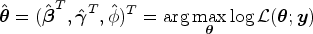
where $\varphi$ is the dispersion parameter, $f_{\mathit{y}|\mathit{b}}({\mathit{y}}_i|{\mathit{b}}_i;\mathit{\theta })$ denotes the conditional density function of ${\mathit{Y}}_i|{\mathit{b}}_i$ , and $f({\mathit{b}}_i;\mathit{\theta })$ denotes the marginal density of ${\mathit{b}}_i$ . Note that the parameters of interest are $\mathit{\beta }$ and $\mathit{\gamma }$ . Define the MLE of $\mathit{\theta }$ by

$$\hat{\mathit{\theta }}=({\hat{\mathit{\beta }}}^T,{\hat{\mathit{\gamma }}}^T,\hat{\varphi }{)}^T=\arg \underset{\mathit{\theta }}{max}\log \mathcal{L}(\mathit{\theta };\mathit{y})$$

Let ${\mathit{\theta }}_0$ denote the true value of $\mathit{\theta }$ . Under mild regularity conditions, $\hat{\mathit{\theta }}$ is consistent and $\sqrt{n}(\hat{\mathit{\theta }}-{\mathit{\theta }}_0)$ ${\to }^D\mathit{N}(\mathbf{0},\mathbf{\Sigma }(\mathit{\theta }))$ , where ${\mathbf{\Sigma }}^{-1}(\mathit{\theta })=\underset{n\to \mathrm{\infty }}{lim}\mathcal{I}(\mathit{\theta })$ , $\mathcal{I}(\mathit{\theta })$ $=-n^{-1}{\mathrm{\partial }}^2\log \mathcal{L}(\mathit{\theta };\mathit{y})/\mathrm{\partial }\mathit{\theta }\mathrm{\partial }{\mathit{\theta }}^T$ , and $\mathbf{\Sigma }(\mathit{\theta })$ is consistently estimated by $\hat{\mathbf{\Sigma }}={\mathcal{I}}^{-1}(\hat{\mathit{\theta }})$ .^28,29

3. Proposed regularized estimations

3.1. Construction of objective function

Variable selection using regularized approach has achieved much success in recent decades. Typically, the objective function is constructed from the observed data likelihood function plus the penalty functions for model parameters. Let

$$Q^o(\mathit{\theta })=-\log \mathcal{L}(\mathit{\theta };\mathit{y})+n{\kappa }_{\rho }^o(\mathit{\beta })+n{\kappa }_{\tau }^o(\mathit{\gamma })$$

and define the regularized estimator ${\hat{\mathit{\theta }}}_{\rho \tau }^o$ = $\arg \underset{\mathit{\theta }}{min}{Q}^o(\mathit{\theta })$ , where ${\kappa }_{\rho }^o(\mathit{\beta })$ and ${\kappa }_{\tau }^o(\mathit{\gamma })$ are penalty terms that control the sparsity for the estimates of $\mathit{\beta }$ and $\mathit{\gamma }$ to select appropriate fixed effects and random effects, respectively. Because the integral in $\mathcal{L}(\mathit{\theta };\mathit{y})$ generally does not have a closed-form solution, various approaches have been proposed to tackle this computational challenge to estimate $\mathit{\theta }$ , including the methods for the commonly used GLMM estimations,^14,15,18 and the methods for the regularized LMM or GLMM estimations.^6,10,12,19 To alleviate such a computational complexity in the regularized estimation process, we propose to perform the regularized estimation by optimizing the objective function constructed from the confidence distribution based on the MLE $\hat{\mathit{\theta }}$ .

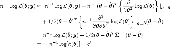
Inference based on the confidence distribution has been extensively studied in the statistical literature (see literary works^30,20,31 and the references therein for a comprehensive review). In short, a confidence distribution can be viewed as a sample dependent distribution function that can be used to estimate and provide all aspects of statistical inference for a parameter of interest. This useful feature has been applied in Liu, Liu and Xie ²⁴ for meta-analysis and Tian, Wang and Cai et al. ²⁵ for joint inference about a set of constrained parameters in survival analysis. Then, based on Singh, Xie and Strawderman ²⁰ and Liu et al., ²⁴ we write the confidence density of the parameter $\mathit{\theta }$ according to the asymptotic distribution of $\hat{\mathit{\theta }}$ :

$$\begin{gathered} h(\mathit{\theta })=\frac{1}{(2\pi {)}^{p/2}{\{det\left(n^{-1}\hat{\mathbf{\Sigma }}\right)\}}^{1/2}} \\ \times \exp \{-\frac{1}{2}(\hat{\mathit{\theta }}-\mathit{\theta }{)}^T{\left(n^{-1}\hat{\mathbf{\Sigma }}\right)}^{-1}(\hat{\mathit{\theta }}-\mathit{\theta })\} \end{gathered}$$

(3)

where $p$ denotes the length of $\mathit{\theta }$ and $det(\mathbf{C}\mathbf{)}$ is the determinant of a matrix $\mathbf{C}$ . Note that $h(\mathit{\theta })$ is a multivariate normal density. Taking the logarithm of $h(\mathit{\theta })$ , we get

$$-\log [h(\mathit{\theta })]=\frac{1}{2}(\hat{\mathit{\theta }}-\mathit{\theta }{)}^T{\left(n^{-1}\hat{\mathbf{\Sigma }}\right)}^{-1}(\hat{\mathit{\theta }}-\mathit{\theta })+c$$

(4)

where $c$ is some constant free of $\mathit{\theta }$ . Consider the following approximation. It can be seen that

$$\begin{array}{rl}{n}^{-1}\log \mathcal{L}(\mathit{\theta };\mathit{y})& \approx n^{-1}\log \mathcal{L}(\hat{\mathit{\theta }};\mathit{y})+n^{-1}(\mathit{\theta }-\hat{\mathit{\theta }}{)}^T\{\frac{\mathrm{\partial }}{\mathrm{\partial }{\mathit{\theta }}^T}\log \mathcal{L}(\mathit{\theta })\}{|}_{\mathit{\theta }\mathbf{=}\hat{\mathit{\theta }}}\\ & +1/2(\mathit{\theta }-\hat{\mathit{\theta }}{)}^T\{n^{-1}\frac{{\mathrm{\partial }}^2}{\mathrm{\partial }\mathit{\theta }\mathrm{\partial }{\mathit{\theta }}^T}\log \mathcal{L}(\mathit{\theta })\}{|}_{\mathit{\theta }\mathbf{=}\hat{\mathit{\theta }}}(\mathit{\theta }-\hat{\mathit{\theta }})\\ & =n^{-1}\log \mathcal{L}(\hat{\mathit{\theta }};\mathit{y})+1/2(\mathit{\theta }-\hat{\mathit{\theta }}{)}^T{\hat{\mathbf{\Sigma }}}^{-1}(\mathit{\theta }-\hat{\mathit{\theta }})\\ & =-n^{-1}\log [h(\mathit{\theta })]+c^{\mathrm{\prime }}\end{array}$$

since $\mathrm{\partial }\log \mathcal{L}(\mathit{\theta };\mathit{y})/\mathrm{\partial }\mathit{\theta }{|}_{\mathit{\theta }=\hat{\mathit{\theta }}}=0$ and constant $c^{\mathrm{\prime }}$ $=n^{-1}\log \mathcal{L}(\hat{\mathit{\theta }};\mathit{y})-c$ is free of $\mathit{\theta }$ . Thus $n^{-1}{Q}^o(\mathit{\theta })\approx n^{-1}\log [h(\mathit{\theta })]+{\kappa }_{\rho }^o(\mathit{\beta })+{\kappa }_{\tau }^o(\mathit{\gamma })+c^{\mathrm{\prime }}$ . This motivates us to construct the following objective function $Q(\mathit{\theta })$ to approximate $Q^o(\mathit{\theta })$ to perform regularized estimation using the confidence density $-\log [h(\mathit{\theta })]$ in (4). Specifically, let

$$Q(\mathit{\theta })=(\hat{\mathit{\theta }}-\mathit{\theta }{)}^T{\left(n^{-1}\hat{\mathbf{\Sigma }}\right)}^{-1}(\hat{\mathit{\theta }}-\mathit{\theta })+n{\kappa }_{\rho }(\mathit{\beta })+n{\kappa }_{\tau }(\mathit{\gamma })$$

(5)

where ${\kappa }_{\rho }(\mathit{\beta })$ and ${\kappa }_{\tau }(\mathit{\gamma })$ are penalty functions. Note that the objective function $Q(\mathit{\theta })$ takes the same form as the objective function of the least squares approximation (LSA) approach proposed by Wang and Leng ³² for the generalized linear models. Define the regularized estimator by

$${\hat{\mathit{\theta }}}_{\rho \tau }=\arg \underset{\mathit{\theta }}{min}Q(\mathit{\theta })$$

(6)

It is interesting to notice the connection of our method with some methods that estimate $\mathit{\theta }$ by optimizing $Q^o(\mathit{\theta })$ . For instance, Ibrahim et al. ¹⁰ estimates $\mathit{\theta }$ by optimizing $Q^o(\mathit{\theta })$ using a Monte Carlo EM algorithm that involves a Markov chain Monte Carlo sampling approach to approximate $\log \mathcal{L}(\mathit{\theta };\mathit{y})$ ; Hui et al. (2017) uses a quasi-likelihood to approximate $\log \mathcal{L}(\mathit{\theta };\mathit{y})$ to estimate $\mathit{\theta }$ . Our method approximates $\log \mathcal{L}(\mathit{\theta };\mathit{y})$ using the log confidence density, $-\log [h(\mathit{\theta })]$ , to estimate $\mathit{\theta }$ . Note that, in our method, performing the numerical approximation of the integration in $\log \mathcal{L}(\mathit{\theta };\mathit{y})$ is only required to derive $\hat{\mathit{\theta }}$ and $\hat{\mathbf{\Sigma }}$ , which can be achieved using existing software packages (e.g. Proc Glimmix in SAS, and lme4 package in R). Once $\hat{\mathit{\theta }}$ and $\hat{\mathbf{\Sigma }}$ are obtained, constructing and optimizing $Q(\mathit{\theta })$ to estimate $\mathit{\theta }$ no longer involves the numerical integration in $\log \mathcal{L}(\mathit{\theta };\mathit{y})$ . Thus, the computational burden is greatly alleviated and the computational efficiency is much improved. In Sections 4 and 5, we discuss how to perform the optimization of $Q(\mathit{\theta })$ using existing software packages and demonstrate the computational efficiency of our method using simulation studies.

3.2. Statistical properties of the proposed estimator

To facilitate statistical inference (e.g. deriving the confidence intervals (CIs)), one may consider to use the adaptive LASSO ³³ or the smoothly clipped absolute deviation (SCAD) ³⁴ penalty functions for ${\kappa }_{\rho }(\cdot )$ and ${\kappa }_{\tau }(\cdot )$ . In this paper, we focus on the adaptive LASSO framework. With little effort, SCAD regularization can be adopted in our proposed procedure. To be specific, we consider the following objective function:

$$Q(\mathit{\theta })=(\hat{\mathit{\theta }}-\mathit{\theta }{)}^T{\left(n^{-1}\hat{\mathbf{\Sigma }}\right)}^{-1}(\hat{\mathit{\theta }}-\mathit{\theta })+n(\sum _{f=1}^{p_f}{\rho }_f|{\beta }_f|+\sum _{m=2}^{p_r+1}{\tau }_m||{\mathit{\gamma }}_m||)$$

by choosing the adaptive LASSO with ${\kappa }_{\rho }(\mathit{\beta })=\sum _{f=1}^{p_f}{\rho }_f|{\beta }_f|$ for the fixed effect selection, where ${\rho }_f^{\mathrm{\prime }}s$ are the adaptive weights that control the penalty with respect to $|{\beta }_f|$ , for $f=1,2,\dots ,p_f$ . For the random-effect selection, we use the adaptive group LASSO, following the rationale by He et al. ³⁵ : Let ${\mathit{\gamma }}_m$ denote the $m$ th row of $\mathbf{\Gamma }$ , then ${\mathit{\gamma }}_m{\mathit{\gamma }}_m^T={\mathit{D}}_{mm}$ which is the $m$ th variance component of the random effects $\mathbf{\Gamma }{\mathit{b}}_i$ , for $m=1,2,\dots ,p_r+1$ . Note that ${\mathit{\gamma }}_m=0\iff {\mathit{D}}_{mm}=$ ${\mathit{D}}_{mh}={\mathit{D}}_{hm}=0$ for all $h$ ; that is, if ${\mathit{\gamma }}_m=0$ , then the variance and covariance elements of $\mathbf{\Gamma }{\mathit{b}}_i$ involving $(\mathbf{\Gamma }{\mathit{b}}_i{)}_m$ are also $0$ . As a result, if a row vector ${\mathit{\gamma }}_m$ is not selected, the random effect $(\mathbf{\Gamma }{\mathit{b}}_i{)}_m$ and the corresponding component in $\mathit{z}$ are excluded from the model and the positive-definitiveness of $\mathit{D}$ is preserved. Thus, the adaptive group LASSO penalty is chosen as ${\kappa }_{\tau }(\mathit{\gamma })=\sum _{m=2}^{p_r+1}{\tau }_m||{\mathit{\gamma }}_m||$ and ${\tau }_m^{\mathrm{\prime }}s$ are the adaptive weights corresponding to $||{\mathit{\gamma }}_m||$ , where $||\mathbf{\cdot }||$ denotes the $L_2$ norm of a vector. Note that the summation starts from $m=2$ to keep the random intercept and preserve the within-subject correlation. Moreover, the parameter $\mathit{\gamma }$ can be expressed as $\mathit{\gamma }=({\gamma }_1,{\mathit{\gamma }}_2^T,\dots ,{\mathit{\gamma }}_m^T{)}^T$ .

Without loss of generality, we assume that only the first $f_0$ fixed effect covariates ${\mathit{x}}_{ij}$ and the first $r_0$ random effect covariates ${\mathit{z}}_{ij}$ , both including the intercepts, are informative. Therefore, we write the true value of $\mathit{\theta }$ by ${\mathit{\theta }}_0=({\mathit{\beta }}_0^T,{\mathit{\gamma }}_0^T,\varphi {)}^T$ , where ${\mathit{\beta }}_0=({\mathit{\beta }}_{0a}^T,{\mathit{\beta }}_{0b}^T={\mathbf{0}}^T)$ and ${\mathit{\gamma }}_0=({\mathit{\gamma }}_{0a}^T,{\mathit{\gamma }}_{0b}^T={\mathbf{0}}^T)$ such that ${\mathit{\beta }}_{0a}=({\beta }_{01},{\beta }_{02},\dots ,{\beta }_{0,f_0}{)}^T$ with ${\beta }_{0j}\ne 0$ for $j=1,2,\dots ,f_0$ , and ${\mathit{\gamma }}_{0a}$ corresponds to the first $r_0$ rows in the lower triangle of $\mathbf{\Gamma }$ and each of these $r_0$ row vectors is non-zero. Similarly, ${\hat{\mathit{\theta }}}_{\rho \tau }=({\hat{\mathit{\beta }}}_{\rho \tau }^T,{\hat{\mathit{\gamma }}}_{\rho \tau }^T,{\hat{\varphi }}_{\rho \tau }{)}^T$ , ${\hat{\mathit{\beta }}}_{\rho \tau }=({\hat{\mathit{\beta }}}_{\rho \tau ,a}^T,{\hat{\mathit{\beta }}}_{\rho \tau ,b}^T{)}^T$ , and ${\hat{\mathit{\gamma }}}_{\rho \tau }=({\hat{\mathit{\gamma }}}_{\rho \tau ,a}^T,{\hat{\mathit{\gamma }}}_{\rho \tau ,b}^T{)}^T$ .

Obviously, $Q(\mathit{\theta })$ is strictly convex in $\mathit{\theta }$ . We establish the consistency and oracle properties of ${\hat{\mathit{\theta }}}_{\rho \tau }$ in Theorem 1.

Theorem 1

Let $a_{f,n}=max\{{\rho }_j,j\le f_0\}$ , $b_{f,n}=min\{{\rho }_j,j>f_0\}$ , $a_{r,n}=max\{{\tau }_j,j\le r_0\}$ , and $b_{r,n}=min\{{\tau }_j,j>r_0\}$ . Then the regularized estimator ${\hat{\mathit{\theta }}}_{\rho \tau }$ satisfies the following as $n\to \mathrm{\infty }$ :

1. (1)

(Estimation consistency) If $n^{1/2}{a}_{f,n}\stackrel{P}{\to }0$ and $n^{1/2}{a}_{r,n}\stackrel{P}{\to }0$ , ${\hat{\mathit{\theta }}}_{\rho \tau }\stackrel{P}{\to }{\mathit{\theta }}_0$ ;

(2)

(Selection consistency) If $n^{1/2}{a}_{f,n}\stackrel{P}{\to }0$ , $n^{1/2}{a}_{r,n}\stackrel{P}{\to }0$ , $n^{1/2}{b}_{f,n}\stackrel{P}{\to }\mathrm{\infty }$ , and $n^{1/2}{b}_{r,n}\stackrel{P}{\to }\mathrm{\infty }$ , Pr $({\hat{\mathit{\beta }}}_{\rho \tau ,b}=\mathbf{0}$ and ${\hat{\mathit{\gamma }}}_{\rho \tau ,b}=\mathbf{0})\to 1$ .

(3)

(Oracle property) Let ${\mathit{\theta }}_{0a}=({\mathit{\beta }}_{0a}^T,{\mathit{\gamma }}_{0a}^T,{\varphi }_0{)}^T$ and ${\hat{\mathit{\theta }}}_{\rho \tau ,a}=({\hat{\mathit{\beta }}}_{\rho \tau ,a}^T,{\hat{\mathit{\gamma }}}_{\rho \tau ,a}^T,{\hat{\varphi }}_0{)}^T$ . If $n^{1/2}{a}_{f,n}\stackrel{P}{\to }0$ , $n^{1/2}{a}_{r,n}\stackrel{P}{\to }0$ , $n^{1/2}{b}_{f,n}\stackrel{P}{\to }\mathrm{\infty }$ , and $n^{1/2}{b}_{r,n}\stackrel{P}{\to }\mathrm{\infty }$ , then $n^{1/2}({\hat{\mathit{\theta }}}_{\rho \tau a}-{\mathit{\theta }}_{0a})\stackrel{D}{\to }\mathcal{N}(\mathbf{0},[({\mathbf{\Sigma }}^{-1}{)}_{{\mathit{\theta }}_{0a}}{]}^{-1})$ , where $({\mathbf{\Sigma }}^{-1}{)}_{{\mathit{\theta }}_{0a}}$ is the submatrix of ${\mathbf{\Sigma }\mathbf{(}\mathit{\theta }\mathbf{)}}^{-1}$ corresponding to true non-zero ${\mathit{\theta }}_{0a}$ . The variance $[({\mathbf{\Sigma }}^{-1}{)}_{{\mathit{\theta }}_{0a}}{]}^{-1}$ can be consistently estimated by $[{\widehat{(\mathbf{\Sigma }}}^{-1}{)}_{{\mathit{\theta }}_{0a}}{]}^{-1}$ , where ${\widehat{(\mathbf{\Sigma }}}^{-1}{)}_{{\mathit{\theta }}_{0a}}$ is the submatrix of ${\hat{\mathbf{\Sigma }}}^{-1}$ corresponding to ${\mathit{\theta }}_{0a}$ .

A sketch of the proof is provided in the Appendix.

3.3. An alternative estimation

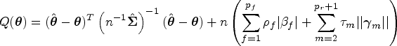
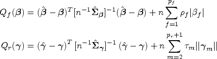
Recall that the objective function $Q(\mathit{\theta })$ is built by the confidence density $h(\mathit{\theta })$ in (3), according to the joint asymptotic distribution of $\hat{\mathit{\theta }}$ . Note that $h(\mathit{\theta })$ is a multivariate normal density. The true values of the means in the joint distribution are the same as those in the marginal distributions. Therefore, we propose another estimation based on the marginal confidence densities with respective to $\mathit{\beta }$ and $\mathit{\gamma }$ in (3) to separately estimate $\mathit{\beta }$ and $\mathit{\gamma }$ . These marginal confidence densities correspond to the marginal asymptotic distributions of the MLEs $\hat{\mathit{\beta }}$ and $\hat{\mathit{\gamma }}$ , respectively. We refer the previous estimation as the CD-joint estimation, and the following estimation as the CD-separate estimation. To proceed, we propose to construct separate objective functions for $\hat{\mathit{\beta }}$ and $\hat{\mathit{\gamma }}$ in the following:

$$\begin{array}{rl}{Q}_f(\mathit{\beta })& =(\hat{\mathit{\beta }}-\mathit{\beta }{)}^T[n^{-1}{\hat{\mathbf{\Sigma }}}_{\mathit{\beta }}{]}^{-1}(\hat{\mathit{\beta }}-\mathit{\beta })+n\sum _{f=1}^{p_f}{\rho }_f|{\beta }_f|\\ Q_r(\mathit{\gamma })& ={(\hat{\mathit{\gamma }}-\mathit{\gamma })}^T[n^{-1}{\hat{\mathbf{\Sigma }}}_{\mathit{\gamma }}{]}^{-1}(\hat{\mathit{\gamma }}-\mathit{\gamma })+n\sum _{m=2}^{p_r+1}{\tau }_m||{\mathit{\gamma }}_m||\end{array}$$

where ${\hat{\mathbf{\Sigma }}}_{\mathit{\beta }}$ and ${\hat{\mathbf{\Sigma }}}_{\mathit{\gamma }}$ are submatrices of $\hat{\mathbf{\Sigma }}$ corresponding to the marginal variance-covariance of $\hat{\mathit{\beta }}$ and $\hat{\mathit{\gamma }}$ , respectively. Define the regularized estimators as ${\hat{\mathit{\beta }}}_{\rho }^s$ = $\arg \underset{\mathit{\beta }}{min}{Q}_f(\mathit{\beta })$ and ${\hat{\mathit{\gamma }}}_{\tau }^s$ = $\arg \underset{\mathit{\gamma }}{min}{Q}_r(\mathit{\gamma })$ . The CD-separate estimation allows for the flexibility of performing the selection of fixed effects only or the selection of random effects only, and enables the performance of fixed- and (or) random-effect selections in case only $\hat{\mathit{\beta }},{\hat{\mathbf{\Sigma }}}_{\mathit{\beta }}$ , $\hat{\mathit{\gamma }},$ and ${\hat{\mathbf{\Sigma }}}_{\mathit{\gamma }}$ are available by convenience.

As noted previously, the true values of the underlying parameters $\mathit{\beta }$ and $\mathit{\gamma }$ in the joint distribution of $\hat{\mathit{\beta }}$ and $\hat{\mathit{\gamma }}$ in $h(\mathit{\theta })$ are the same as those in the individual marginal distributions of $\hat{\mathit{\beta }}$ and $\hat{\mathit{\gamma }}$ in $h(\mathit{\theta })$ , respectively. Therefore, the true values of $\mathit{\beta }$ and $\mathit{\gamma }$ for the estimators based on the CD-joint estimation and CD-separate estimation are the same, although the CD-joint estimators and CD-separate estimators are different estimators. Recall that ${\mathit{\beta }}_0$ and ${\mathit{\gamma }}_0$ are expressed as ${\mathit{\beta }}_0=({\mathit{\beta }}_{0a}^T,{\mathit{\beta }}_{0b}^T={\mathbf{0}}^T{)}^T$ and ${\mathit{\gamma }}_0=({\mathit{\gamma }}_{0a}^T,{\mathit{\gamma }}_{0b}^T={\mathbf{0}}^T{)}^T$ . Similarly, we write ${\hat{\mathit{\beta }}}_{\rho }^s=({\hat{\mathit{\beta }}}_{\rho ,a}^s{}^T,{\hat{\mathit{\beta }}}_{\rho ,b}^s{}^T{)}^T$ and ${\hat{\mathit{\gamma }}}_{\tau }^s=({\hat{\mathit{\gamma }}}_{\tau ,a}^s{}^T,{{\hat{\mathit{\gamma }}}_{\tau ,b}^s{}^T)}^T$ . Obviously, both $Q_f(\mathit{\beta })$ and $Q_r(\mathit{\gamma })$ are convex in $\mathit{\beta }$ and $\mathit{\gamma }$ , respectively. We establish the consistency and oracle properties for ${\hat{\mathit{\beta }}}_{\rho }^s$ and ${\hat{\mathit{\gamma }}}_{\tau }^s$ as follows.

Theorem 2

Let $a_{f,n}=max\{{\rho }_j,j\le f_0\}$ , and $b_{f,n}=min\{{\rho }_j,j>f_0\}$ . Then the regularized estimator ${\hat{\mathit{\beta }}}_{\rho }^s$ satisfies the following as $n\to \mathrm{\infty }$ :

1. (1)

(Estimation consistency) If $n^{1/2}{a}_{f,n}\stackrel{P}{\to }0$ , ${\hat{\mathit{\beta }}}_{\rho }^s\stackrel{P}{\to }{\mathit{\beta }}_0$ ;

(2)

(Selection consistency) If $n^{1/2}{a}_{f,n}\stackrel{P}{\to }0$ , and $n^{1/2}{b}_{f,n}\stackrel{P}{\to }\mathrm{\infty }$ , Pr $({\hat{\mathit{\beta }}}_{\rho ,b}^s=\mathbf{0})\to 1$ .

(3)

(Oracle property) If $n^{1/2}{a}_{f,n}\stackrel{P}{\to }0$ , and $n^{1/2}{b}_{f,n}\stackrel{P}{\to }\mathrm{\infty }$ , then $n^{1/2}({\hat{\mathit{\beta }}}_{\rho ,a}^s-{\mathit{\beta }}_{0a})\stackrel{D}{\to }\mathcal{N}(\mathbf{0},[({\mathbf{\Sigma }}_{\mathit{\beta }}^{-1}{)}_{{\mathit{\beta }}_{0a}}{]}^{-1})$ , where $({\mathbf{\Sigma }}_{\mathit{\beta }}^{-1}{)}_{{\mathit{\beta }}_{0a}}$ is the submatrix of ${\mathbf{\Sigma }}_{\mathit{\beta }}^{-1}$ corresponding to ${\mathit{\beta }}_{0a}$ . The variance $[({\mathbf{\Sigma }}_{\mathit{\beta }}^{-1}{)}_{{\mathit{\beta }}_{0a}}{]}^{-1}$ can be consistently estimated by $[({\hat{\mathbf{\Sigma }}}_{\mathit{\beta }}^{-1}{)}_{{\mathit{\beta }}_{0a}}{]}^{-1}$ , where ${\widehat{({\mathbf{\Sigma }}_{\mathit{\beta }}}}^{-1}{)}_{{\mathit{\beta }}_{0a}}$ is the submatrix of ${\hat{\mathbf{\Sigma }}}_{\mathit{\beta }}^{-1}$ corresponding to ${\mathit{\beta }}_{0a}$ .

Theorem 3

Let $a_{r,n}=max\{{\tau }_j,j\le r_0\}$ , and $b_{r,n}=min\{{\tau }_j,j>r_0\}$ . Then the regularized estimator ${\hat{\mathit{\gamma }}}_{\tau }^s$ satisfies the following as $n\to \mathrm{\infty }$ :

1. (1)

(Estimation consistency) If $n^{1/2}{a}_{r,n}\stackrel{P}{\to }0$ , ${\hat{\mathit{\gamma }}}_{\tau }^s\stackrel{P}{\to }{\mathit{\gamma }}_0$ ;

(2)

(Selection Consistency) If $n^{1/2}{a}_{r,n}\stackrel{P}{\to }0$ , and $n^{1/2}{b}_{r,n}\stackrel{P}{\to }\mathrm{\infty }$ , Pr $({\hat{\mathit{\gamma }}}_{\tau ,b}^s=\mathbf{0}$ $)\to 1$ .

(3)

(Oracle Property) If $n^{1/2}{a}_{r,n}\stackrel{P}{\to }0$ , and $n^{1/2}{b}_{r,n}\stackrel{P}{\to }\mathrm{\infty }$ , then $n^{1/2}({\hat{\mathit{\gamma }}}_{\tau ,a}^s-{\mathit{\gamma }}_{0a})\stackrel{D}{\to }\mathcal{N}(\mathbf{0},[({\mathbf{\Sigma }}_{\mathit{\gamma }}^{-1}{)}_{{\mathit{\gamma }}_{0a}}{]}^{-1})$ , where $({\mathbf{\Sigma }}_{\mathit{\gamma }}^{-1}{)}_{{\mathit{\gamma }}_{0a}}$ is the submatrix of ${\mathbf{\Sigma }}_{\mathit{\gamma }}^{-1}$ corresponding to ${\mathit{\gamma }}_{0a}$ . The variance $[({\mathbf{\Sigma }}_{\mathit{\gamma }}^{-1}{)}_{{\mathit{\gamma }}_{0a}}{]}^{-1}$ can be consistently estimated by $[({\hat{\mathbf{\Sigma }}}_{\mathit{\gamma }}^{-1}{)}_{{\mathit{\gamma }}_{0a}}{]}^{-1}$ , where ${\widehat{({\mathbf{\Sigma }}_{\mathit{\gamma }}}}^{-1}{)}_{{\mathit{\gamma }}_{0a}}$ is the submatrix of ${\hat{\mathbf{\Sigma }}}_{\mathit{\gamma }}^{-1}$ corresponding to ${\mathit{\gamma }}_{0a}$ .

The proofs for Theorems 2 and 3 are similar to that for Theorem 1, thus are omitted.

Although the dispersion parameter $\varphi$ is often a nuisance parameter and thus omitted in the previously described separate estimation, it can actually be included, for instance, by combining $\varphi$ with $\mathit{\gamma }$ . Then we modify $Q_r(\mathit{\gamma })$ by $Q_r^{*}(\mathit{\gamma },\varphi )$ given below, based on the (marginal) joint distribution of $\hat{\mathit{\gamma }}$ and $\hat{\varphi }$ in (3):

$$Q_r^{*}(\mathit{\gamma },\varphi )={\left(\begin{array}{c}\hat{\mathit{\gamma }}-\mathit{\gamma }\\ \hat{\varphi }-\varphi \end{array}\right)}^T[n^{-1}{\hat{\mathbf{\Sigma }}}_{\gamma \varphi }{]}^{-1}\left(\begin{array}{c}\hat{\mathit{\gamma }}-\mathit{\gamma }\\ \hat{\varphi }-\varphi \end{array}\right)+n{\kappa }_{\tau }(\mathit{\gamma })$$

where ${\hat{\mathbf{\Sigma }}}_{\gamma \varphi }$ is the variance-covariance of $\hat{\mathit{\gamma }}$ and $\hat{\varphi }$ .

4. Optimization and determination of tuning parameters

To obtain ${\hat{\mathit{\theta }}}_{\rho \tau }$ via optimizing $Q(\mathit{\theta })$ , we follow the method of Zhang and Lu ³⁶ and rewrite the objective function $Q(\mathit{\theta })$ as

$$Q(\mathit{\theta })={(\mathrm{\Lambda }\mathit{\theta }-\mathrm{\Psi })}^T(\mathrm{\Lambda }\mathit{\theta }-\mathrm{\Psi })+n{\kappa }_{\rho }(\mathit{\beta })+n{\kappa }_{\tau }(\mathit{\gamma })$$

(7)

where $\mathrm{\Psi }=\mathrm{\Lambda }\hat{\mathit{\theta }}$ , and $\mathrm{\Lambda }$ can be obtained using the singular value decomposition such that $(n^{-1}\hat{\mathbf{\Sigma }}{)}^{-1}={\mathrm{\Lambda }}^T\mathrm{\Lambda }$ . Then the function in (7) is a typical convex optimization problem and can be solved by standard software packages, for instance, the R packages glmnet ³⁷ and gglasso. ³⁸ The same approach can also be applied to optimize $Q_f(\mathit{\beta })$ , $Q_r(\mathit{\gamma })$ , and $Q_r^{*}(\mathit{\gamma }\mathbf{,}\varphi )$ . For instance, let ${\mathrm{\Psi }}_{\mathit{\beta }}={\mathrm{\Lambda }}_{\mathit{\beta }}\hat{\mathit{\beta }}$ and ${\mathrm{\Psi }}_{\mathit{\gamma }}={\mathrm{\Lambda }}_{\mathit{\gamma }}\hat{\mathit{\gamma }}$ , where ${\mathrm{\Lambda }}_{\mathit{\beta }}$ and ${\mathrm{\Lambda }}_{\mathit{\gamma }}$ are obtained using the singular value decomposition such that $[n^{-1}{\hat{\mathbf{\Sigma }}}_{\mathit{\beta }}{]}^{-1}={\mathrm{\Lambda }}_{\mathit{\beta }}^T{\mathrm{\Lambda }}_{\mathit{\beta }}$ and $[n^{-1}{\hat{\mathbf{\Sigma }}}_{\mathit{\gamma }}{]}^{-1}={\mathrm{\Lambda }}_{\mathit{\gamma }}^T{\mathrm{\Lambda }}_{\mathit{\gamma }}$ . As a result, $Q_f(\mathit{\beta })=({\mathrm{\Lambda }}_{\mathit{\beta }}\mathit{\beta }-{\mathrm{\Psi }}_{\mathit{\beta }}{)}^T({\mathrm{\Lambda }}_{\mathit{\beta }}\mathit{\beta }-{\mathrm{\Psi }}_{\mathit{\beta }})+n{\kappa }_{\rho }(\mathit{\beta })$ and $Q_r(\mathit{\gamma })=({\mathrm{\Lambda }}_{\mathit{\gamma }}\mathit{\gamma }-{\mathrm{\Psi }}_{\mathit{\gamma }}{)}^T({\mathrm{\Lambda }}_{\mathit{\gamma }}\mathit{\gamma }-{\mathrm{\Psi }}_{\mathit{\gamma }})+n{\kappa }_{\tau }(\mathit{\gamma })$ , respectively. In our simulations and data analysis, we used R package gglasso to optimize $Q(\mathit{\theta })$ , $Q_r(\mathit{\gamma })$ , and $Q_r^{*}(\mathit{\gamma },\varphi )$ , and glmnet to optimize $Q_f(\mathit{\beta })$ .

Typically, the tuning parameters ${\rho }_f$ ’s and ${\tau }_m$ ’s can be chosen using the approaches of cross validation or generalized cross validation. But, these methods can be computationally extensive. With the simple solution suggested by Zou, ³³ we consider ${\rho }_f=\lambda |{\hat{\beta }}_f{|}^{-{\phi }_f}$ and ${\tau }_m=\lambda ||{\hat{\mathit{\gamma }}}_m|{|}^{-{\phi }_r}$ for the CD-joint estimation method, and ${\rho }_f={\lambda }_f|{\hat{\beta }}_f{|}^{-{\phi }_f}$ and ${\tau }_m={\lambda }_r||{\hat{\mathit{\gamma }}}_m|{|}^{-{\phi }_r}$ for the CD-separate estimation method, for $f=1,2,\dots ,p_f$ and $m=2,3,\dots ,p_r+1$ , where ${\hat{\beta }}_f$ and ${\hat{\mathit{\gamma }}}_m$ are the maximum likelihood estimates for ${\beta }_f$ and ${\gamma }_m$ , respectively, and ${\phi }_f$ and ${\phi }_r$ are pre-specified positive numbers. In the CD-joint method, the adaptive LASSO penalties for the fixed effects and random effects are linked by the tuning parameter $\lambda >0$ . The CD-separate estimation allows each of the fixed- and random-effect selections to have its own tuning parameter to control the shrinkage. Because the MLEs ${\hat{\beta }}_f$ ’s and ${\hat{\mathit{\gamma }}}_m$ ’s are $\sqrt{n}$ -consistent, it can be verified that the tuning parameters considered above satisfy the conditions required by Theorems 1, 2, and 3, provided that $n^{1/2}\lambda \to 0$ , $n^{(1+{\phi }_f)/2}\lambda \to \mathrm{\infty }$ , and $n^{(1+{\phi }_r)/2}\lambda \to \mathrm{\infty }$ as well as $n^{1/2}{\lambda }_f\to 0$ , $n^{(1+{\phi }_f)/2}{\lambda }_f\to \mathrm{\infty }$ , $n^{1/2}{\lambda }_r\to 0$ and $n^{(1+{\phi }_r)/2}{\lambda }_r\to \mathrm{\infty }$ . Thus it suffices to select $\lambda \in R+=[0,\mathrm{\infty })$ , ${\lambda }_f\in R+=[0,\mathrm{\infty })$ and ${\lambda }_r\in R+=[0,\mathrm{\infty })$ . Therefore, to determine $\lambda$ , ${\lambda }_f$ , and ${\lambda }_r$ , we consider to minimize BIC, per recommendations by prior research.^32,40 Specifically, for the CD-joint estimation, we define the BIC as: $BI{C}_{\rho \tau }=n({\hat{\mathit{\theta }}}_{\rho \tau }-\hat{\mathit{\theta }}{)}^T{\hat{\mathbf{\Sigma }}}^{-1}({\hat{\mathit{\theta }}}_{\rho \tau }-\hat{\mathit{\theta }})+(\log n)(d{f}_{\rho }+d{f}_{\tau }),$ where $d{f}_{\rho }$ is the number of non-zero coefficients in ${\hat{\mathit{\beta }}}_{\rho \tau }$ , and $d{f}_{\tau }$ is the number of groups with non-zero within-group coefficients ${\hat{\mathit{\gamma }}}_{\rho \tau }$ . For the CD-separate estimation, we define $BI{C}_{f,\rho }=n({\hat{\mathit{\beta }}}_{\rho }^s-\hat{\mathit{\beta }}{)}^T{\hat{\mathbf{\Sigma }}}_{\mathit{\beta }}^{-1}({\hat{\mathit{\beta }}}_{\rho }^s-\hat{\mathit{\beta }})+(\log n)d{f}_{\rho }$ for optimizing $Q_f(\mathit{\beta })$ , and $BI{C}_{r,\tau }=n({\hat{\mathit{\gamma }}}_{\tau }^s-\hat{\mathit{\gamma }}{)}^T{\hat{\mathbf{\Sigma }}}_{\mathit{\gamma }}^{-1}({\hat{\mathit{\gamma }}}_{\tau }^s-\hat{\mathit{\gamma }})+(\log n)d{f}_{\tau }$ and $BI{C}_{r,\tau }^{*}=(\begin{array}{c}\hat{\mathit{\gamma }}-\mathit{\gamma }\\ \hat{\varphi }-\varphi \end{array}{)}^T[n^{-1}{\hat{\mathbf{\Sigma }}}_{\gamma \varphi }{]}^{-1}(\begin{array}{c}\hat{\mathit{\gamma }}-\mathit{\gamma }\\ \hat{\varphi }-\varphi \end{array})+(\log n)d{f}_{\tau }$ for optimizing $Q_r(\mathit{\gamma })$ and $Q_r^{*}(\mathit{\gamma }\mathbf{,}\varphi )$ , respectively.

5. Simulation studies

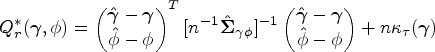
We conducted simulation studies to examine the performance of the proposed CD methods and compared them with the methods by Hui et al. ¹⁹ (rpql R package), Bondell et al. ⁶ (available at https://blogs.unimelb.edu.au/howard-bondell/), and the method of Groll et al. ¹¹ (glmmLasso R package). Hui et al. ¹⁹ and Bondell et al. ⁶ used adaptive Lasso penalties. Groll et al. ¹¹ used the Lasso penalty. We applied these methods because either the R packages or the R code are publicly available. Data were simulated under 3 scenarios (i.e. LMM, random effects logistic regression models, and random effects Poisson models) according to model (1), with results summarized in Tables 1 to 5. Moreover, we have extended our methods to nested random effects in GLMM, with detailed descriptions of model specifications and simulation results in the Supplemental Materials.

Table 1.

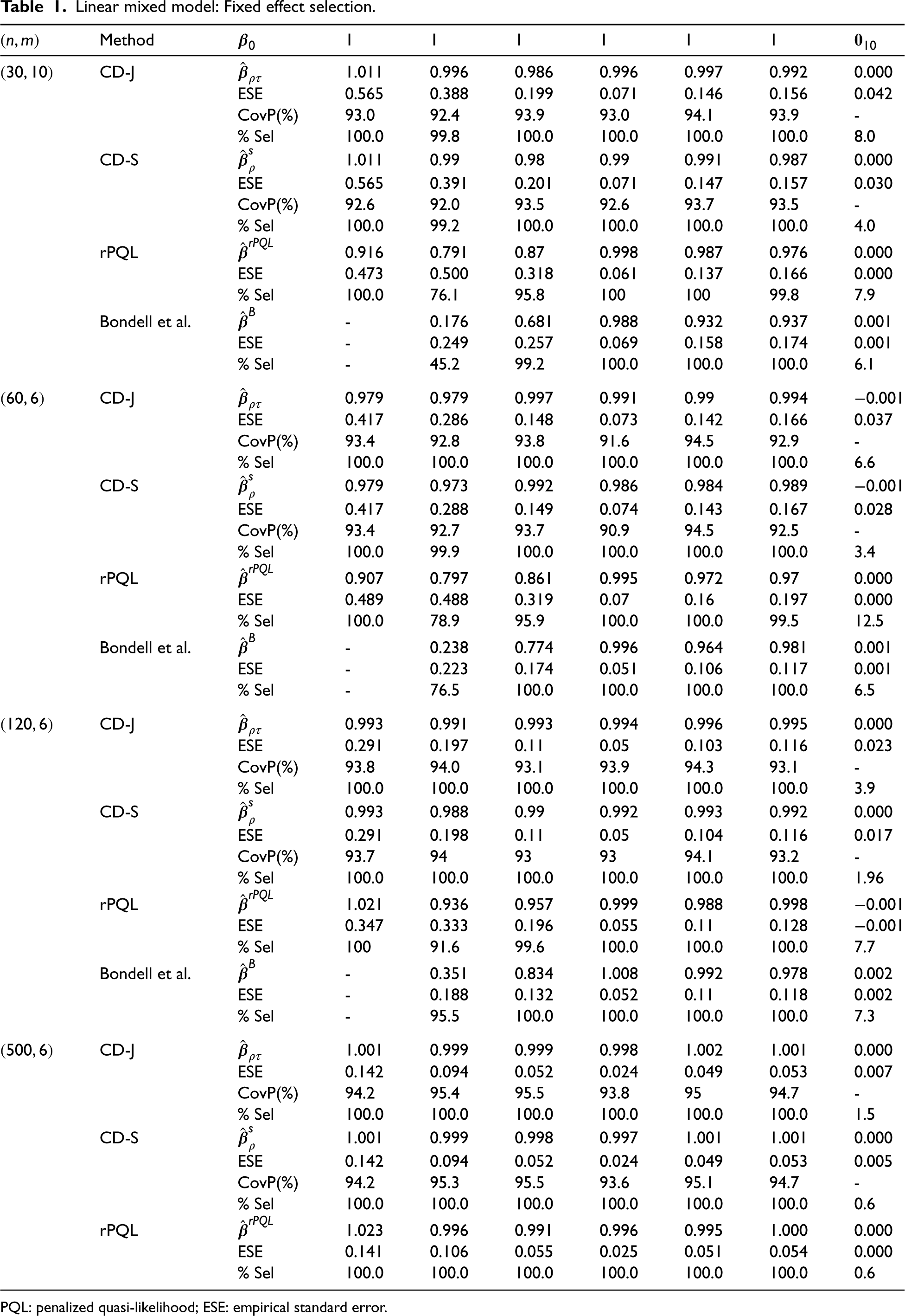
Linear mixed model: Fixed effect selection.

$(n,m)$	Method	${\mathit{\beta }}_0$	1	1	1	1	1	1	${\mathbf{0}}_{10}$
$(30,10)$	CD-J	${\hat{\mathit{\beta }}}_{\rho \tau }$	1.011	0.996	0.986	0.996	0.997	0.992	0.000
		ESE	0.565	0.388	0.199	0.071	0.146	0.156	0.042
		CovP(%)	93.0	92.4	93.9	93.0	94.1	93.9	-
		% Sel	100.0	99.8	100.0	100.0	100.0	100.0	8.0
	CD-S	${\hat{\mathit{\beta }}}_{\rho }^s$	1.011	0.99	0.98	0.99	0.991	0.987	0.000
		ESE	0.565	0.391	0.201	0.071	0.147	0.157	0.030
		CovP(%)	92.6	92.0	93.5	92.6	93.7	93.5	-
		% Sel	100.0	99.2	100.0	100.0	100.0	100.0	4.0
	rPQL	${\hat{\mathit{\beta }}}^{rPQL}$	0.916	0.791	0.87	0.998	0.987	0.976	0.000
		ESE	0.473	0.500	0.318	0.061	0.137	0.166	0.000
		% Sel	100.0	76.1	95.8	100	100	99.8	7.9
	Bondell et al.	${\hat{\mathit{\beta }}}^B$	-	0.176	0.681	0.988	0.932	0.937	0.001
		ESE	-	0.249	0.257	0.069	0.158	0.174	0.001
		% Sel	-	45.2	99.2	100.0	100.0	100.0	6.1
$(60,6)$	CD-J	${\hat{\mathit{\beta }}}_{\rho \tau }$	0.979	0.979	0.997	0.991	0.99	0.994	$-$ 0.001
		ESE	0.417	0.286	0.148	0.073	0.142	0.166	0.037
		CovP(%)	93.4	92.8	93.8	91.6	94.5	92.9	-
		% Sel	100.0	100.0	100.0	100.0	100.0	100.0	6.6
	CD-S	${\hat{\mathit{\beta }}}_{\rho }^s$	0.979	0.973	0.992	0.986	0.984	0.989	$-$ 0.001
		ESE	0.417	0.288	0.149	0.074	0.143	0.167	0.028
		CovP(%)	93.4	92.7	93.7	90.9	94.5	92.5	-
		% Sel	100.0	99.9	100.0	100.0	100.0	100.0	3.4
	rPQL	${\hat{\mathit{\beta }}}^{rPQL}$	0.907	0.797	0.861	0.995	0.972	0.97	0.000
		ESE	0.489	0.488	0.319	0.07	0.16	0.197	0.000
		% Sel	100.0	78.9	95.9	100.0	100.0	99.5	12.5
	Bondell et al.	${\hat{\mathit{\beta }}}^B$	-	0.238	0.774	0.996	0.964	0.981	0.001
		ESE	-	0.223	0.174	0.051	0.106	0.117	0.001
		% Sel	-	76.5	100.0	100.0	100.0	100.0	6.5
$(120,6)$	CD-J	${\hat{\mathit{\beta }}}_{\rho \tau }$	0.993	0.991	0.993	0.994	0.996	0.995	0.000
		ESE	0.291	0.197	0.11	0.05	0.103	0.116	0.023
		CovP(%)	93.8	94.0	93.1	93.9	94.3	93.1	-
		% Sel	100.0	100.0	100.0	100.0	100.0	100.0	3.9
	CD-S	${\hat{\mathit{\beta }}}_{\rho }^s$	0.993	0.988	0.99	0.992	0.993	0.992	0.000
		ESE	0.291	0.198	0.11	0.05	0.104	0.116	0.017
		CovP(%)	93.7	94	93	93	94.1	93.2	-
		% Sel	100.0	100.0	100.0	100.0	100.0	100.0	1.96
	rPQL	${\hat{\mathit{\beta }}}^{rPQL}$	1.021	0.936	0.957	0.999	0.988	0.998	$-$ 0.001
		ESE	0.347	0.333	0.196	0.055	0.11	0.128	$-$ 0.001
		% Sel	100	91.6	99.6	100.0	100.0	100.0	7.7
	Bondell et al.	${\hat{\mathit{\beta }}}^B$	-	0.351	0.834	1.008	0.992	0.978	0.002
		ESE	-	0.188	0.132	0.052	0.11	0.118	0.002
		% Sel	-	95.5	100.0	100.0	100.0	100.0	7.3
$(500,6)$	CD-J	${\hat{\mathit{\beta }}}_{\rho \tau }$	1.001	0.999	0.999	0.998	1.002	1.001	0.000
		ESE	0.142	0.094	0.052	0.024	0.049	0.053	0.007
		CovP(%)	94.2	95.4	95.5	93.8	95	94.7	-
		% Sel	100.0	100.0	100.0	100.0	100.0	100.0	1.5
	CD-S	${\hat{\mathit{\beta }}}_{\rho }^s$	1.001	0.999	0.998	0.997	1.001	1.001	0.000
		ESE	0.142	0.094	0.052	0.024	0.049	0.053	0.005
		CovP(%)	94.2	95.3	95.5	93.6	95.1	94.7	-
		% Sel	100.0	100.0	100.0	100.0	100.0	100.0	0.6
	rPQL	${\hat{\mathit{\beta }}}^{rPQL}$	1.023	0.996	0.991	0.996	0.995	1.000	0.000
		ESE	0.141	0.106	0.055	0.025	0.051	0.054	0.000
		% Sel	100.0	100.0	100.0	100.0	100.0	100.0	0.6

PQL: penalized quasi-likelihood; ESE: empirical standard error.

Table 2.

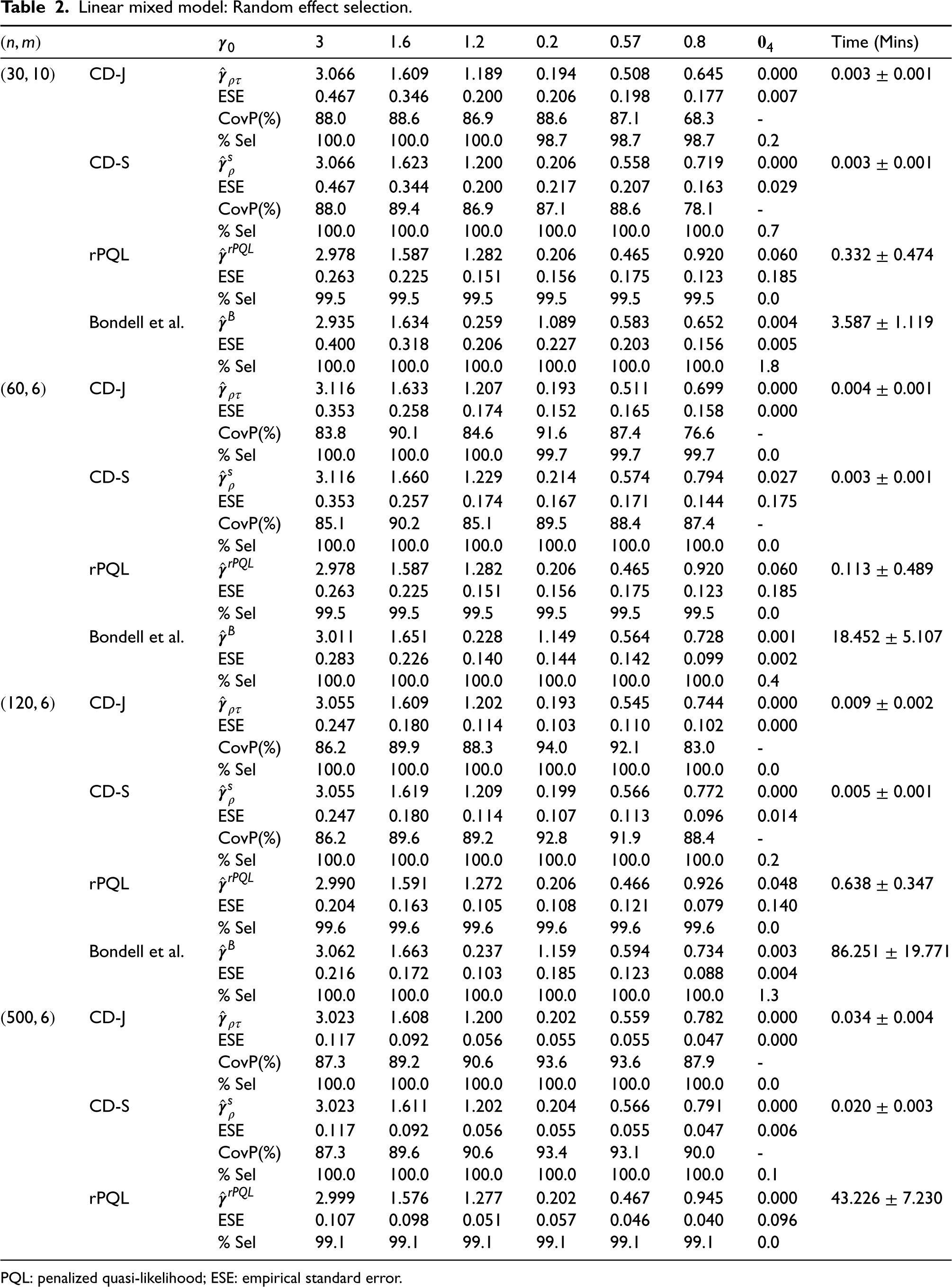
Linear mixed model: Random effect selection.

$(n,m)$		${\mathit{\gamma }}_0$	3	1.6	1.2	0.2	0.57	0.8	${\mathbf{0}}_4$	Time (Mins)
$(30,10)$	CD-J	${\hat{\mathit{\gamma }}}_{\rho \tau }$	3.066	1.609	1.189	0.194	0.508	0.645	0.000	0.003 $\pm$ 0.001
		ESE	0.467	0.346	0.200	0.206	0.198	0.177	0.007
		CovP(%)	88.0	88.6	86.9	88.6	87.1	68.3	-
		% Sel	100.0	100.0	100.0	98.7	98.7	98.7	0.2
	CD-S	${\hat{\mathit{\gamma }}}_{\rho }^s$	3.066	1.623	1.200	0.206	0.558	0.719	0.000	0.003 $\pm$ 0.001
		ESE	0.467	0.344	0.200	0.217	0.207	0.163	0.029
		CovP(%)	88.0	89.4	86.9	87.1	88.6	78.1	-
		% Sel	100.0	100.0	100.0	100.0	100.0	100.0	0.7
	rPQL	${\hat{\mathit{\gamma }}}^{rPQL}$	2.978	1.587	1.282	0.206	0.465	0.920	0.060	0.332 $\pm$ 0.474
		ESE	0.263	0.225	0.151	0.156	0.175	0.123	0.185
		% Sel	99.5	99.5	99.5	99.5	99.5	99.5	0.0
	Bondell et al.	${\hat{\mathit{\gamma }}}^B$	2.935	1.634	0.259	1.089	0.583	0.652	0.004	3.587 $\pm$ 1.119
		ESE	0.400	0.318	0.206	0.227	0.203	0.156	0.005
		% Sel	100.0	100.0	100.0	100.0	100.0	100.0	1.8
$(60,6)$	CD-J	${\hat{\mathit{\gamma }}}_{\rho \tau }$	3.116	1.633	1.207	0.193	0.511	0.699	0.000	0.004 $\pm$ 0.001
		ESE	0.353	0.258	0.174	0.152	0.165	0.158	0.000
		CovP(%)	83.8	90.1	84.6	91.6	87.4	76.6	-
		% Sel	100.0	100.0	100.0	99.7	99.7	99.7	0.0
	CD-S	${\hat{\mathit{\gamma }}}_{\rho }^s$	3.116	1.660	1.229	0.214	0.574	0.794	0.027	0.003 $\pm$ 0.001
		ESE	0.353	0.257	0.174	0.167	0.171	0.144	0.175
		CovP(%)	85.1	90.2	85.1	89.5	88.4	87.4	-
		% Sel	100.0	100.0	100.0	100.0	100.0	100.0	0.0
	rPQL	${\hat{\mathit{\gamma }}}^{rPQL}$	2.978	1.587	1.282	0.206	0.465	0.920	0.060	0.113 $\pm$ 0.489
		ESE	0.263	0.225	0.151	0.156	0.175	0.123	0.185
		% Sel	99.5	99.5	99.5	99.5	99.5	99.5	0.0
	Bondell et al.	${\hat{\mathit{\gamma }}}^B$	3.011	1.651	0.228	1.149	0.564	0.728	0.001	18.452 $\pm$ 5.107
		ESE	0.283	0.226	0.140	0.144	0.142	0.099	0.002
		% Sel	100.0	100.0	100.0	100.0	100.0	100.0	0.4
$(120,6)$	CD-J	${\hat{\mathit{\gamma }}}_{\rho \tau }$	3.055	1.609	1.202	0.193	0.545	0.744	0.000	0.009 $\pm$ 0.002
		ESE	0.247	0.180	0.114	0.103	0.110	0.102	0.000
		CovP(%)	86.2	89.9	88.3	94.0	92.1	83.0	-
		% Sel	100.0	100.0	100.0	100.0	100.0	100.0	0.0
	CD-S	${\hat{\mathit{\gamma }}}_{\rho }^s$	3.055	1.619	1.209	0.199	0.566	0.772	0.000	0.005 $\pm$ 0.001
		ESE	0.247	0.180	0.114	0.107	0.113	0.096	0.014
		CovP(%)	86.2	89.6	89.2	92.8	91.9	88.4	-
		% Sel	100.0	100.0	100.0	100.0	100.0	100.0	0.2
	rPQL	${\hat{\mathit{\gamma }}}^{rPQL}$	2.990	1.591	1.272	0.206	0.466	0.926	0.048	0.638 $\pm$ 0.347
		ESE	0.204	0.163	0.105	0.108	0.121	0.079	0.140
		% Sel	99.6	99.6	99.6	99.6	99.6	99.6	0.0
	Bondell et al.	${\hat{\mathit{\gamma }}}^B$	3.062	1.663	0.237	1.159	0.594	0.734	0.003	86.251 $\pm$ 19.771
		ESE	0.216	0.172	0.103	0.185	0.123	0.088	0.004
		% Sel	100.0	100.0	100.0	100.0	100.0	100.0	1.3
$(500,6)$	CD-J	${\hat{\mathit{\gamma }}}_{\rho \tau }$	3.023	1.608	1.200	0.202	0.559	0.782	0.000	0.034 $\pm$ 0.004
		ESE	0.117	0.092	0.056	0.055	0.055	0.047	0.000
		CovP(%)	87.3	89.2	90.6	93.6	93.6	87.9	-
		% Sel	100.0	100.0	100.0	100.0	100.0	100.0	0.0
	CD-S	${\hat{\mathit{\gamma }}}_{\rho }^s$	3.023	1.611	1.202	0.204	0.566	0.791	0.000	0.020 $\pm$ 0.003
		ESE	0.117	0.092	0.056	0.055	0.055	0.047	0.006
		CovP(%)	87.3	89.6	90.6	93.4	93.1	90.0	-
		% Sel	100.0	100.0	100.0	100.0	100.0	100.0	0.1
	rPQL	${\hat{\mathit{\gamma }}}^{rPQL}$	2.999	1.576	1.277	0.202	0.467	0.945	0.000	43.226 $\pm$ 7.230
		ESE	0.107	0.098	0.051	0.057	0.046	0.040	0.096
		% Sel	99.1	99.1	99.1	99.1	99.1	99.1	0.0

PQL: penalized quasi-likelihood; ESE: empirical standard error.

Table 3.

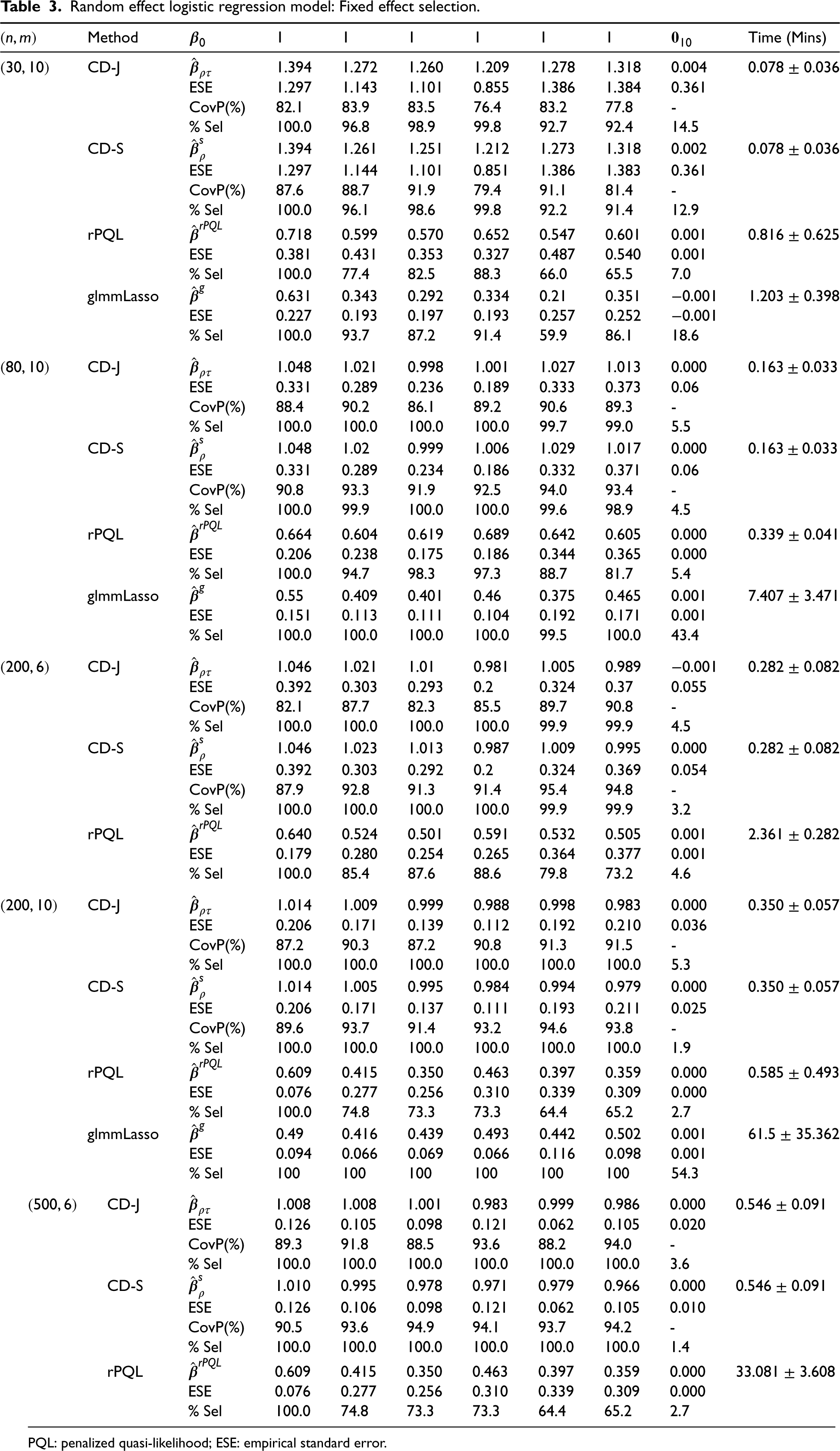
Random effect logistic regression model: Fixed effect selection.

$(n,m)$	Method	${\mathit{\beta }}_0$	1	1	1	1	1	1	${\mathbf{0}}_{10}$	Time (Mins)
$(30,10)$	CD-J	${\hat{\mathit{\beta }}}_{\rho \tau }$	1.394	1.272	1.260	1.209	1.278	1.318	0.004	0.078 $\pm$ 0.036
		ESE	1.297	1.143	1.101	0.855	1.386	1.384	0.361
		CovP(%)	82.1	83.9	83.5	76.4	83.2	77.8	-
		% Sel	100.0	96.8	98.9	99.8	92.7	92.4	14.5
	CD-S	${\hat{\mathit{\beta }}}_{\rho }^s$	1.394	1.261	1.251	1.212	1.273	1.318	0.002	0.078 $\pm$ 0.036
		ESE	1.297	1.144	1.101	0.851	1.386	1.383	0.361
		CovP(%)	87.6	88.7	91.9	79.4	91.1	81.4	-
		% Sel	100.0	96.1	98.6	99.8	92.2	91.4	12.9
	rPQL	${\hat{\mathit{\beta }}}^{rPQL}$	0.718	0.599	0.570	0.652	0.547	0.601	0.001	0.816 $\pm$ 0.625
		ESE	0.381	0.431	0.353	0.327	0.487	0.540	0.001
		% Sel	100.0	77.4	82.5	88.3	66.0	65.5	7.0
	glmmLasso	${\hat{\mathit{\beta }}}^g$	0.631	0.343	0.292	0.334	0.21	0.351	$-$ 0.001	1.203 $\pm$ 0.398
		ESE	0.227	0.193	0.197	0.193	0.257	0.252	$-$ 0.001
		% Sel	100.0	93.7	87.2	91.4	59.9	86.1	18.6
$(80,10)$	CD-J	${\hat{\mathit{\beta }}}_{\rho \tau }$	1.048	1.021	0.998	1.001	1.027	1.013	0.000	$0.163\pm 0.033$
		ESE	0.331	0.289	0.236	0.189	0.333	0.373	0.06
		CovP(%)	88.4	90.2	86.1	89.2	90.6	89.3	-
		% Sel	100.0	100.0	100.0	100.0	99.7	99.0	5.5
	CD-S	${\hat{\mathit{\beta }}}_{\rho }^s$	1.048	1.02	0.999	1.006	1.029	1.017	0.000	$0.163\pm 0.033$
		ESE	0.331	0.289	0.234	0.186	0.332	0.371	0.06
		CovP(%)	90.8	93.3	91.9	92.5	94.0	93.4	-
		% Sel	100.0	99.9	100.0	100.0	99.6	98.9	4.5
	rPQL	${\hat{\mathit{\beta }}}^{rPQL}$	0.664	0.604	0.619	0.689	0.642	0.605	0.000	0.339 $\pm$ 0.041
		ESE	0.206	0.238	0.175	0.186	0.344	0.365	0.000
		% Sel	100.0	94.7	98.3	97.3	88.7	81.7	5.4
	glmmLasso	${\hat{\mathit{\beta }}}^g$	0.55	0.409	0.401	0.46	0.375	0.465	0.001	7.407 $\pm$ 3.471
		ESE	0.151	0.113	0.111	0.104	0.192	0.171	0.001
		% Sel	100.0	100.0	100.0	100.0	99.5	100.0	43.4
$(200,6)$	CD-J	${\hat{\mathit{\beta }}}_{\rho \tau }$	1.046	1.021	1.01	0.981	1.005	0.989	$-$ 0.001	0.282 $\pm$ 0.082
		ESE	0.392	0.303	0.293	0.2	0.324	0.37	0.055
		CovP(%)	82.1	87.7	82.3	85.5	89.7	90.8	-
		% Sel	100.0	100.0	100.0	100.0	99.9	99.9	4.5
	CD-S	${\hat{\mathit{\beta }}}_{\rho }^s$	1.046	1.023	1.013	0.987	1.009	0.995	0.000	0.282 $\pm$ 0.082
		ESE	0.392	0.303	0.292	0.2	0.324	0.369	0.054
		CovP(%)	87.9	92.8	91.3	91.4	95.4	94.8	-
		% Sel	100.0	100.0	100.0	100.0	99.9	99.9	3.2
	rPQL	${\hat{\mathit{\beta }}}^{rPQL}$	0.640	0.524	0.501	0.591	0.532	0.505	0.001	2.361 $\pm$ 0.282
		ESE	0.179	0.280	0.254	0.265	0.364	0.377	0.001
		% Sel	100.0	85.4	87.6	88.6	79.8	73.2	4.6
$(200,10)$	CD-J	${\hat{\mathit{\beta }}}_{\rho \tau }$	1.014	1.009	0.999	0.988	0.998	0.983	0.000	0.350 $\pm$ 0.057
		ESE	0.206	0.171	0.139	0.112	0.192	0.210	0.036
		CovP(%)	87.2	90.3	87.2	90.8	91.3	91.5	-
		% Sel	100.0	100.0	100.0	100.0	100.0	100.0	5.3
	CD-S	${\hat{\mathit{\beta }}}_{\rho }^s$	1.014	1.005	0.995	0.984	0.994	0.979	0.000	0.350 $\pm$ 0.057
		ESE	0.206	0.171	0.137	0.111	0.193	0.211	0.025
		CovP(%)	89.6	93.7	91.4	93.2	94.6	93.8	-
		% Sel	100.0	100.0	100.0	100.0	100.0	100.0	1.9
	rPQL	${\hat{\mathit{\beta }}}^{rPQL}$	0.609	0.415	0.350	0.463	0.397	0.359	0.000	0.585 $\pm$ 0.493
		ESE	0.076	0.277	0.256	0.310	0.339	0.309	0.000
		% Sel	100.0	74.8	73.3	73.3	64.4	65.2	2.7
	glmmLasso	${\hat{\mathit{\beta }}}^g$	0.49	0.416	0.439	0.493	0.442	0.502	0.001	61.5 $\pm$ 35.362
		ESE	0.094	0.066	0.069	0.066	0.116	0.098	0.001
		% Sel	100	100	100	100	100	100	54.3
$(500,6)$	CD-J	${\hat{\mathit{\beta }}}_{\rho \tau }$	1.008	1.008	1.001	0.983	0.999	0.986	0.000	0.546 $\pm$ 0.091
		ESE	0.126	0.105	0.098	0.121	0.062	0.105	0.020
		CovP(%)	89.3	91.8	88.5	93.6	88.2	94.0	-
		% Sel	100.0	100.0	100.0	100.0	100.0	100.0	3.6
	CD-S	${\hat{\mathit{\beta }}}_{\rho }^s$	1.010	0.995	0.978	0.971	0.979	0.966	0.000	0.546 $\pm$ 0.091
		ESE	0.126	0.106	0.098	0.121	0.062	0.105	0.010
		CovP(%)	90.5	93.6	94.9	94.1	93.7	94.2	-
		% Sel	100.0	100.0	100.0	100.0	100.0	100.0	1.4
	rPQL	${\hat{\mathit{\beta }}}^{rPQL}$	0.609	0.415	0.350	0.463	0.397	0.359	0.000	33.081 $\pm$ 3.608
		ESE	0.076	0.277	0.256	0.310	0.339	0.309	0.000
		% Sel	100.0	74.8	73.3	73.3	64.4	65.2	2.7

PQL: penalized quasi-likelihood; ESE: empirical standard error.

Table 4.

Random effect logistic regression model: Random effect selection.

$(n,m)$	Method	${\mathit{\gamma }}_0$	1.73	0.69	1.23	0.46	0.15	0.88	${\mathbf{0}}_4$
$(30,10)$	CD-J	${\hat{\mathit{\gamma }}}_{\rho \tau }$	2.181	0.662	1.139	0.324	0.018	0.339	0.003
		ESE	1.284	1.023	1.657	0.738	0.549	1.472	0.297
		CovP $(\mathrm{\%})$	79.9	81.9	73.1	27.5	23.9	27.9	-
		% Sel	100.0	86.0	86.0	32.7	32.7	32.7	1.6
	CD-S	${\hat{\mathit{\gamma }}}_{\tau }^s$	2.181	0.770	1.375	0.476	0.074	0.493	0.003
		ESE	1.284	1.047	1.629	0.839	0.662	1.507	0.297
		CovP $(\mathrm{\%})$	89.0	88.5	91.2	44.5	40.4	45.4	-
		% Sel	100.0	96.2	96.2	50.5	50.5	49.2	1.6
	rPQL	${\hat{\mathit{\gamma }}}^{rPQL}$	1.127	0.421	0.651	0.300	0.126	0.261	0.000
		ESE	0.070	0.105	0.133	0.132	0.194	0.170	0.014
		% Sel	90.0	86.6	87.7	69.4	68.5	70.8	60.1
$(80,10)$	CD-J	${\hat{\mathit{\gamma }}}_{\rho \tau }$	1.761	0.617	1.037	0.316	0.060	0.455	0.000
		ESE	0.293	0.289	0.299	0.315	0.212	0.403	0.000
		CovP $(\mathrm{\%})$	87.9	91.4	77.4	61.8	61.3	60.5	-
		% Sel	100.0	99.6	99.6	63.6	63.6	63.6	0.0
	CD-S	${\hat{\mathit{\gamma }}}_{\tau }^s$	1.761	0.677	1.145	0.417	0.096	0.632	0.000
		ESE	0.293	0.301	0.288	0.340	0.271	0.419	0.000
		CovP $(\mathrm{\%})$	92.9	94.0	88.6	74.7	73.2	76.8	-
		% Sel	100.0	100.0	100.0	78.1	78.1	78.0	0.0
	rPQL	${\hat{\mathit{\gamma }}}^{rPQL}$	1.108	0.416	0.597	0.291	0.091	0.235	0.006
		ESE	0.180	0.211	0.212	0.222	0.281	0.220	0.156
		% Sel	99.3	97.3	97.3	84.3	84.0	84.3	41.4
$(200,6)$	CD-J	${\hat{\mathit{\gamma }}}_{\rho \tau }$	1.740	0.636	1.031	0.356	0.067	0.507	0.000
		ESE	0.250	0.242	0.287	0.315	0.205	0.407	0.006
		CovP $(\mathrm{\%})$	83.2	89.3	69.5	63.4	66.3	65.5	-
		% Sel	100.0	99.9	99.9	68.7	68.7	68.7	0.1
	CD-S	${\hat{\mathit{\gamma }}}_{\tau }^s$	1.740	0.695	1.127	0.456	0.103	0.666	0.000
		ESE	0.250	0.248	0.278	0.326	0.257	0.417	0.006
		CovP $(\mathrm{\%})$	92.0	93.3	85.6	76.3	75.8	78.4	-
		% Sel	100.0	99.9	99.9	81.0	81.0	81.0	0.1
	rPQL	${\hat{\mathit{\gamma }}}^{rPQL}$	1.108	0.416	0.597	0.291	0.091	0.235	0.006
		ESE	0.180	0.211	0.212	0.222	0.281	0.220	0.156
		% Sel	82.0	74.5	76.5	53.5	53.0	53.5	11.4
$(200,10)$	CD-J	${\hat{\mathit{\gamma }}}_{\rho \tau }$	1.714	0.648	1.117	0.398	0.109	0.672	0.000
		ESE	0.166	0.174	0.173	0.193	0.156	0.235	0.000
		CovP $(\mathrm{\%})$	89.3	92.2	78.5	85.5	91.6	72.9	-
		% Sel	100.0	100.0	100.0	95.2	95.2	95.2	0.0
	CD-S	${\hat{\mathit{\gamma }}}_{\tau }^s$	1.714	0.674	1.167	0.452	0.128	0.779	0.000
		ESE	0.166	0.177	0.169	0.190	0.178	0.201	0.000
		CovP $(\mathrm{\%})$	93.8	93.9	89.2	92.7	92.7	90.9	-
		% Sel	100.0	100.0	100.0	99.4	99.4	99.4	0.0
	rPQL	${\hat{\mathit{\gamma }}}^{rPQL}$	1.108	0.416	0.597	0.291	0.091	0.235	0.006
		ESE	0.180	0.211	0.212	0.222	0.281	0.220	0.156
		% Sel	99.9	99.4	99.4	85.4	85.7	85.8	20.0
$(500,6)$	CD-J	${\hat{\mathit{\gamma }}}_{\rho \tau }$	1.714	0.648	1.117	0.398	0.109	0.672	0.000
		ESE	0.166	0.174	0.173	0.193	0.156	0.235	0.000
		CovP $(\mathrm{\%})$	89.3	92.2	78.5	85.5	91.6	72.9	-
		% Sel	100.0	100.0	100.0	95.2	95.2	95.2	0.0
	CD-S	${\hat{\mathit{\gamma }}}_{\tau }^s$	1.714	0.674	1.167	0.452	0.128	0.779	0.000
		ESE	0.166	0.177	0.169	0.190	0.178	0.201	0.000
		CovP $(\mathrm{\%})$	93.8	93.9	89.2	92.7	92.7	90.9	-
		% Sel	100.0	100.0	100.0	99.4	99.4	99.4	0.0
	rPQL	${\hat{\mathit{\gamma }}}^{rPQL}$	0.985	0.384	0.545	0.245	0.056	0.174	0.000
		ESE	0.093	0.134	0.156	0.242	0.230	0.130	0.000
		% Sel	82.4	71.8	72.9	57.6	56.5	57.6	1.2

PQL: penalized quasi-likelihood; ESE: empirical standard error. ${}^a$ $CovP(\mathrm{\%})$ calculated after excluding incorrect non-selections ( $0$ ’s

Table 5.

Random effects poisson regression model: Fixed effect and random effect selections.

Fixed effects		Method	${\mathit{\beta }}_0$	$1$	$-1$	$-1$	$-1$	$-1$	$-1$	${\mathbf{0}}_{10}$	Time (mins)
	$(30,10)$	CD-J	${\hat{\mathit{\beta }}}_{\rho \tau }$	0.990	$-$ 1.020	$-$ 0.989	$-$ 0.999	$-$ 0.988	$-$ 0.986	0.001	0.113 $\pm$ 0.090
			ESE	0.313	0.292	0.209	0.028	0.098	0.079	0.012
			CovP(%)	94.6	90.3	91.3	86.0	71.9	76.3	-
			% Sel	100.0	100.0	100.0	100.0	100.0	100.0	5.8
		CD-S	${\hat{\mathit{\beta }}}_{\rho }^s$	0.990	$-$ 1.019	$-$ 0.988	$-$ 0.998	$-$ 0.987	$-$ 0.985	0.000	0.113 $\pm$ 0.090
			ESE	0.313	0.292	0.209	0.028	0.098	0.079	0.008
			CovP(%)	94.6	90.6	91.3	86.6	90.6	87.0	-
			% Sel	100.0	100.0	100.0	100.0	100.0	100.0	1.7
		rPQL	${\hat{\mathit{\beta }}}^{rPQL}$	1.107	$-$ 0.964	$-$ 0.938	$-$ 0.996	$-$ 0.989	$-$ 1.001	0.000	0.062 $\pm$ 0.013
			ESE	0.331	0.308	0.271	0.042	0.108	0.119	0.000
			% Sel	100.0	97.9	99.1	100.0	99.9	100.0	0.9
	$(200,6)$	CD-J	${\hat{\mathit{\beta }}}_{\rho \tau }$	0.991	$-$ 1.008	$-$ 1.000	$-$ 1.001	$-$ 1.004	$-$ 1.001	0.000	0.260 $\pm$ 0.197
			ESE	0.135	0.114	0.087	0.014	0.044	0.037	0.004
			CovP(%)	94.3	93.1	93.9	91.0	77.6	87.8	-
			% Sel	100.0	100.0	100.0	100.0	100.0	100.0	2.1
		CD-S	${\hat{\mathit{\beta }}}_{\rho }^s$	0.991	$-$ 1.008	$-$ 1.000	$-$ 1.000	$-$ 1.003	$-$ 1.001	0.000	0.260 $\pm$ 0.196
			ESE	0.135	0.114	0.087	0.014	0.044	0.037	0.003
			CovP(%)	94.7	93.1	94.7	91.8	95.9	93.9	-
			% Sel	100.0	100.0	100.0	100.0	100.0	100.0	0.8
		rPQL	${\hat{\mathit{\beta }}}^{rPQL}$	1.000	$-$ 1.000	$-$ 1.006	$-$ 0.998	$-$ 0.997	$-$ 0.999	0.000	2.971 $\pm$ 0.716
			ESE	0.135	0.113	0.100	0.013	0.027	0.030	0.000
			% Sel	100.0	100.0	100.0	100.0	100.0	100.0	0.2
	$(500,6)$	CD-J	${\hat{\mathit{\beta }}}_{\rho \tau }$	1.000	$-$ 1.000	$-$ 0.997	$-$ 1.000	$-$ 1.003	$-$ 1.002	0.000	0.565 $\pm$ 0.190
			ESE	0.079	0.064	0.056	0.007	0.029	0.022	0.002
			CovP(%)	94.9	97.7	92.2	95.9	75.1	85.3	-
			% Sel	100.0	100.0	100.0	100.0	100.0	100.0	0.7
		CD-S	${\hat{\mathit{\beta }}}_{\rho }^s$	1.000	$-$ 0.999	$-$ 0.997	$-$ 1.000	$-$ 1.003	$-$ 1.002	0.000	0.565 $\pm$ 0.190
			ESE	0.079	0.064	0.056	0.007	0.029	0.022	0.001
			CovP(%)	94.9	97.7	92.2	96.3	94.9	91.7	-
			% Sel	100.0	100.0	100.0	100.0	100.0	100.0	0.2
		rPQL	${\hat{\mathit{\beta }}}^{rPQL}$	1.009	$-$ 1.003	$-$ 0.999	$-$ 0.999	$-$ 0.999	$-$ 0.998	0.000	43.025 $\pm$ 7.323
			ESE	0.082	0.067	0.056	0.016	0.018	0.007	0.000
			% Sel	100.0	100.0	100.0	100.0	100.0	100.0	100.0
Random effects			${\mathit{\gamma }}_0$	1.73	0.69	1.23	0.46	0.15	0.88	${\mathbf{0}}_4$
	$(30,10)$	CD-J	${\hat{\mathit{\gamma }}}_{\rho \tau }$	1.703	0.679	1.136	0.416	0.136	0.722	0.000
			ESE	0.267	0.257	0.163	0.204	0.185	0.135	0.000
			CovP(%)	89.6	92.3	84.3	91.0	90.6	73.2	0.0
			% Sel	100.0	100.0	100.0	100.0	100.0	100.0	-
		CD-S	${\hat{\mathit{\gamma }}}_{\rho }^s$	1.703	0.693	1.165	0.445	0.147	0.800	0.000
			ESE	0.267	0.260	0.163	0.212	0.198	0.132	0.000
			CovP(%)	89.6	94.3	88.3	93.6	89.0	86.0	-
			% Sel	100.0	100.0	100.0	100.0	100.0	100.0	0.0
		rPQL	${\hat{\mathit{\gamma }}}^{rPQL}$	1.573	0.631	1.143	0.387	0.156	0.761	0.001
			ESE	0.247	0.276	0.176	0.233	0.197	0.168	0.034
			% Sel	100.0	100.0	100.0	100.0	100.0	100.0	0.0
	$(200,6)$	CD-J	${\hat{\mathit{\gamma }}}_{\rho \tau }$	1.727	0.684	1.216	0.453	0.138	0.839	0.000
			ESE	0.101	0.106	0.074	0.085	0.075	0.063	0.001
			CovP(%)	95.5	93.9	89.8	95.1	94.7	85.3	-
			% Sel	100.0	100.0	100.0	100.0	100.0	100.0	0.0
		CD-S	${\hat{\mathit{\gamma }}}_{\rho }^s$	1.727	0.688	1.224	0.461	0.141	0.859	0.000
			ESE	0.101	0.107	0.074	0.086	0.077	0.061	0.001
			CovP(%)	95.5	95.1	90.2	96.7	93.5	89.8	-
			% Sel	100.0	100.0	100.0	100.0	100.0	100.0	0.0
		rPQL	${\hat{\mathit{\gamma }}}^{rPQL}$	1.626	0.652	1.191	0.426	0.155	0.842	0.000
			ESE	0.093	0.106	0.072	0.086	0.078	0.060	0.000
			% Sel	99.8	99.8	99.8	99.8	99.8	99.8	0.0
	$(500,6)$	CD-J	${\hat{\mathit{\gamma }}}_{\rho \tau }$	1.716	0.681	1.227	0.446	0.145	0.856	0.000
			ESE	0.067	0.068	0.047	0.060	0.048	0.040	0.000
			CovP(%)	92.2	94.0	94.0	90.8	94.0	88.0	-
			% Sel	100.0	100.0	100.0	100.0	100.0	100.0	0.0
		CD-S	${\hat{\mathit{\gamma }}}_{\rho }^s$	1.716	0.683	1.231	0.450	0.147	0.865	0.000
			ESE	0.067	0.068	0.046	0.061	0.049	0.040	0.000
			CovP(%)	92.2	94.5	95.4	92.6	94.0	90.8	-
			% Sel	100.0	100.0	100.0	100.0	100.0	100.0	0.0
		rPQL	${\hat{\mathit{\gamma }}}^{rPQL}$	1.629	0.652	1.200	0.428	0.148	0.848	0.000
			ESE	0.061	0.065	0.040	0.054	0.047	0.035
			% Sel	99.5	99.5	99.5	99.5	99.5	99.5	0.0

PQL: penalized quasi-likelihood; ESE: empirical standard error.

In Scenario 1, we generated $y_{ij}^{\mathrm{\prime }}s$ from the LMM such that $y_{ij}|{\mathit{b}}_i$ follows $N({\mathit{x}}_{ij}^T\mathit{\beta }+{\mathit{z}}_{ij}^T\mathbf{\Gamma }{\mathit{b}}_i,{\sigma }^2)$ with $\varphi ={\sigma }^2=1$ . In Scenario 2, we simulated binary data from the random effects logistic regression model. In Scenario 3, we simulated count data for the random effects Poisson model with a log link. In all three scenarios, we chose $p_f=15$ for fixed effects and $p_r=3$ for random effects. The true value for $\mathit{\beta }$ was ${\mathit{\beta }}_0=({\mathbf{1}}_6,{\mathbf{0}}_{10})$ for LMM and random effects logistic regression models (Scenarios 1 and 2), and ${\mathit{\beta }}_0=(1,-{\mathbf{1}}_5,{\mathbf{0}}_{10})$ for random effects Poisson models (Scenarios 3). The true $4\times 4$ random effect covariance matrix $\mathit{D}$ is given by $vech(\mathit{D})=(9,4.8,0.6,0;4,0.9,0;1,0;0)$ for Scenario 1, and $vech(\mathit{D})=(3,1.2,0.8,0;2,0.5,0;1,0;0)$ for Scenarios 2 and 3, i.e. only the first three components of ${\mathit{z}}_{ij}$ , including the random intercept, are informative. As a result, we express the corresponding Cholesky decomposition lower triangular matrix by showing the row elements in the lower triangle as $\mathbf{\Gamma }=(3;1.6,1.2;0.2,0.57,0.8;{\mathbf{0}}_4)$ for Scenario 1 and $\mathbf{\Gamma }=(1.73;0.69,1.23;0.46,0.15,0.88;{\mathbf{0}}_4)$ for Scenarios 2 and 3. In each scenario, we considered varying numbers of clusters $n$ and cluster size $m$ . Covariates ${\mathit{x}}_{ij}=(1,x_{ij,1},x_{ij,2},\dots ,x_{ij,p_f}{)}^T$ and ${\mathit{z}}_{ij}=(1,z_{ij,1},z_{ij,2},\dots ,z_{ij,p_r}{)}^T$ , for $p_f=15$ and $p_r=3$ , were generated from a mix of continuous, categorical (binary) variables and interactions of continuous and categorical variables. Specifically, $x_{ij,1},x_{ij,3},x_{ij,6}\sim x_{ij,8}$ are generated from the standard normal distribution, $x_{ij,2},x_{ij,12}\sim x_{ij,14}$ were generated from exponential distribution with mean $1$ (exponential(1)), $x_{ij,4},x_{ij,9}\sim x_{ij,11}$ were generated from Bernoulli (0.4) distribution; $x_{ij,4}$ and $x_{ij,15}$ are interaction terms with $x_{ij,5}=x_{ij,1}*x_{ij,4}$ and $x_{ij,15}=x_{ij,6}*x_{ij,9}$ . Moreover, $z_{ij,l}=x_{ij,l}$ , for $l=1,2,3$ . All continuous covariates were standardized to have mean $0$ and variance $1$ .

For the proposed methods, we refer CD-joint and CD-separate estimations as CD-J and CD-S, respectively. We showed the mean of the estimates, empirical standard error (ESE), percentage of selection (% Sel), and the average computation time (Time (mins)). For the proposed CD methods, coverage probability of 95% CIs (CovP) was calculated based on the oracle properties in Theorems 1 to 3. In addition to the CD methods, we also fitted the GLMM models to obtain the model estimates as initial values to implement the method of Hui et al. ¹⁹ (referred to as the rPQL method), following the examples in Hui. ³⁹ When we calculated the computation time, we included the time for fitting the GLMM models, when applicable, as well as the time of the regularization process, including the determination of tuning parameters. The R lme4 package was used to derive the GLMM estimates. For the CD-J and CD-S, the tuning parameters $\lambda$ , ${\lambda }_f$ , and ${\lambda }_r$ were determined from ${10}^{\omega }$ , where $\omega$ went from $-4$ to $4$ by $0.01$ ( $801$ values in total). For the rPQL method, we used the function $lseq()$ , provided by the rpql package, ³⁹ to determine the tuning parameters from $(0,100]$ using syntax “ $lseq(1e-6,{10}^2,length=200)$ ” (200 values in total). Several ranges wider than $(0,100]$ were applied, each for $50-100$ simulation runs, and results were similar. For glmmLasso, the tuning parameters were chosen from ${10}^{\omega }$ , where $\omega$ went from $-4$ to $4$ by $0.08$ ( $101$ values in total). We applied different ranges and different numbers of tuning parameters for the CD-methods, rPQL and glmmLasso methods, with CD-methods using the most number of tuning parameters. Because the computation time of the rPQL and glmmLasso methods was longer, especially for large $n$ ’s, we determined to use smaller numbers of tuning parameters for these methods to facilitate the progress of the simulation studies, after trying various ranges of tuning parameters and making sure results were similar.

Moreover, we performed additional simulations to examine the impact of ${\phi }_f$ and ${\phi }_r$ (see results in the Supplemental Materials). Specifically, we considered the values of ${\phi }_f$ and ${\phi }_r$ to be $0.25$ , $1$ and $4$ for the proposed CD-J, CD-S, and the rPQL method because the rpql package provided the flexibility to specify the penalty weight. In this section, we reported results of ${\phi }_f$ = ${\phi }_r$ =1 for the CD-J and CD-S methods, and ${\phi }_f$ = ${\phi }_r$ =4 for the rPQL method because of the better performance.

Scenario 1. For LMM, we showed the performance of the proposed CD-J and CD-S methods, and compared them with the rPQL method and Bondell’s method. For the Bondell’s method, we did not show the intercept estimates because they were not readily provided. Also, we did not continue with Bondell’s method for $(n,m)=(500,6)$ because of being unable to complete the estimation process after 48 hours for a single try. For fixed effect selection using the CD-J and CD-S methods (Table 1), results were vey similar. The estimates in both ${\hat{\beta }}_{\rho \tau }$ and ${\hat{\beta }}_{\rho }^s$ were very close to the true values. The types of covariates (e.g. continuous vs. binary, symmetric vs. right-skewed, and interactions) had little impact on the biasedness of the estimates. The ESE, as expected, decreased with $n$ . The coverage probability of 95% CI for the proposed CD-J and CD-S was generally close to the nominal 95% level. For the performance of the variable selection, the selection of true covariates by the CD methods was close to 100%. The noise covariates were selected but at a very low rate, especially for large $n$ . For the rPQL and Bondell’s methods, we noted that the first 3 fixed effect estimates in ${\hat{\beta }}^{rPQL}$ (rPQL) and ${\hat{\beta }}^B$ (Bondell’s method), whose corresponding covariates are associated with random effects, showed some bias from the true values and low selection rate when the number of clusters $n$ is moderately small (e.g. $n=30,60$ ), but the bias and selection rate improved as $n$ increased. For the random effect selections (Table 2), the parameter estimates of the proposed CD methods were generally close to the true values; the ESE decreases with $n$ , and the coverage probability of 95% CI is close to but slightly under the nominal 95% level. The selection rate of true covariates was nearly 100%. The noise covariates were selected but at a very lower rate. The rPQL and Bondell’s methods were similar, too. In terms of the computation time, the CD methods generally took less than ( $\ll$ ) 1 minute, while the other two methods can take much longer, especially when $n$ is large (say, $n=500$ ). When $n$ is moderate to large, the proposed CD methods can be an attractive and competitive approach.

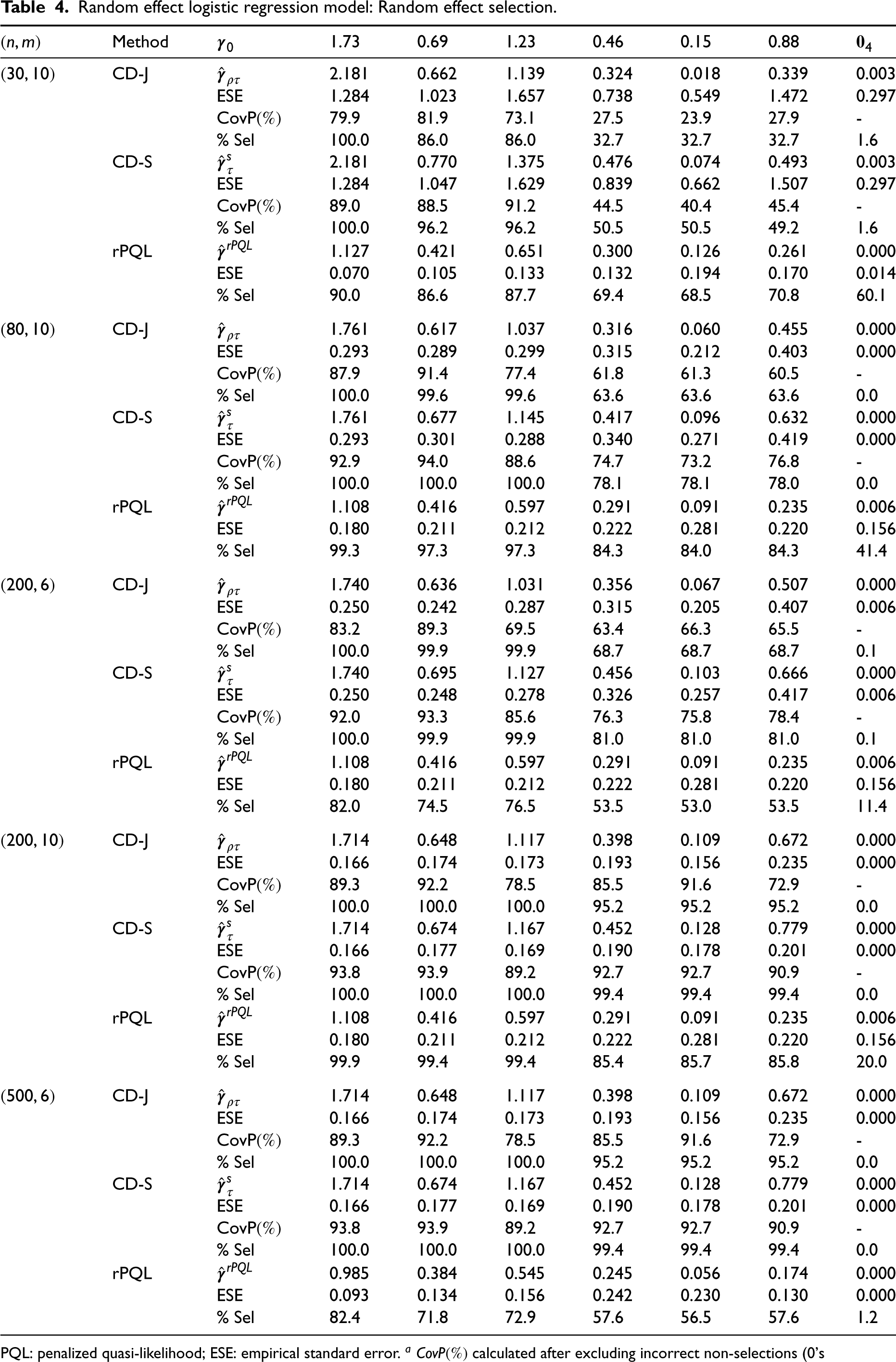
Scenario 2. For the random effects logistic regression models, we compared the CD methods with rPQL and glmmLasso ¹¹ for the fixed effect selection (Table 3). Note that glmmLasso only performs the fixed effect selection. When we used glmmLasso, we included the correct random-effect covariates in the models. For the CD methods, there was some bias in the fixed effect estimates when $n$ is small (e.g. $n=30$ ), but the bias and ESE decreased with $n$ . When $n$ is $80$ or more, the bias becomes minimal. The coverage probability was lower than the nominal 95% level for small $n$ (e.g. $n=30$ ), largely due to the bias of ${\hat{\mathit{\beta }}}_{\rho \tau }$ and ${\hat{\mathit{\beta }}}_{\rho }^s$ , but improved as $n$ increased. The performance of CD-S was slightly better than the CD-J, with a slightly lower false selection rate and better coverage rate of the 95% CI. For both CD methods, the computation time was primarily spent in deriving $\hat{\theta }$ and $\hat{\mathrm{\Sigma }}$ . The time to obtain ${\hat{\beta }}_{\rho \tau }$ , ${\hat{\beta }}_{\rho }^s$ , ${\hat{\gamma }}_{\rho \tau }$ , and ${\hat{\gamma }}_{\rho }^s$ in the regularized estimation process was minimal ( $\ll$ 1 minute). Compared to rPQL and glmmLasso, the bias of the estimates, the selection rate and computation time, the CD methods were obviously better. For the random effect selection (Table 4), results were similar. For the CD methods, there was some bias in the random effect estimates when $n$ is small (e.g. $n=30$ ). When $n$ increased to $80$ or more, the bias became minimal. The selection rate was lower when $n$ was small which resulted in lower coverage rate of the 95% CIs. We also noticed that the selection rate of the random effect corresponding to $x_{ij,2}$ was low. It might be because $x_{ij,2}$ follows the exponential distribution with mean 1 and is right-skewed. After increasing $m$ (e.g. $(n,m)=(200,6)$ increased to $(n,m)=(200,10)$ ) and/or increasing $n$ , the selection rate and the probability coverage rate of the 95% CIs improved. Compared to rPQL, the bias of the estimates and the selection rate of the CD methods were better.

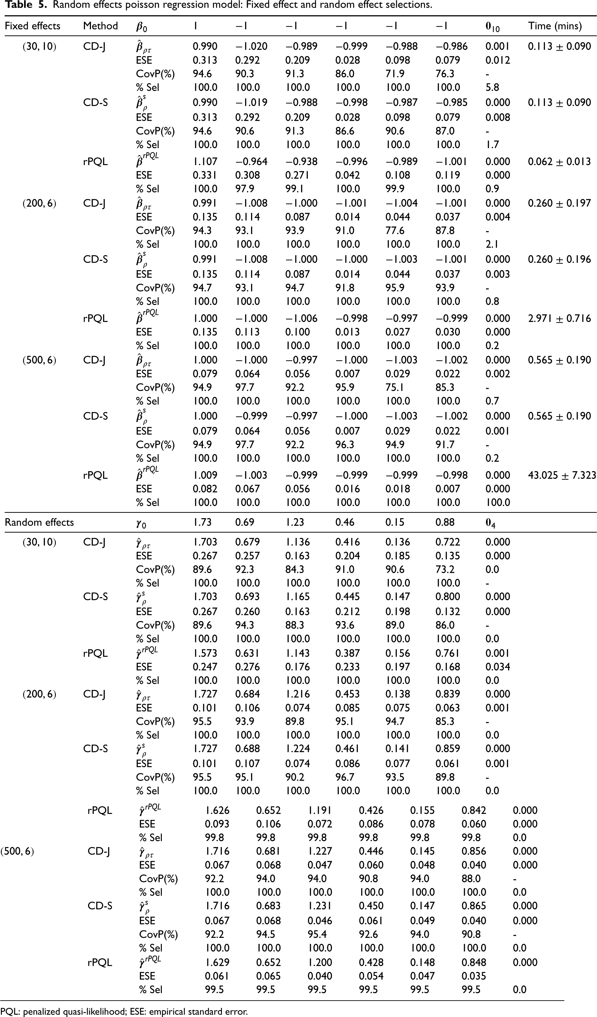
Scenario 3. For the random effects Poisson regression models (Table 5), the fixed effect and random effect estimates of CD-J, CD-S and rPQL methods were very close to the true values. The selection rate of true covariates was close to 100%, and nearly no noise covariates was selected by all three methods. Compared to rPQL, the computation time of the CD methods was shorter, especially when $n$ is large.

6. Applications: Data analysis

We applied the proposed CD approach to the two longitudinal cancer studies that motivated our methods. Regression coefficient estimates were reported and the 95% CIs by the CD methods were calculated based on the oracle properties in Theorems 2 and 3. Moreover, we used ${\phi }_f$ = ${\phi }_r$ =1 in the CD methods, and ${\phi }_f$ = ${\phi }_r$ =4 in the rPQL method, based on the results from simulation studies.

Data Example 1. This study longitudinally measured the tumor volume during the cycles of radiation therapy in 111 patients with unresectable, locally advanced, non-small cell lung cancer (NSCLC). Most patients were treated with concurrent chemoradiation therapy (CRT) as it offers much improved survival outcomes, compared to a sequential combination of chemotherapy followed by radiation therapy. ⁴¹ To measure the response to CRT, the cone beam computed tomography, as part of the image guided radiation therapy and known to have higher precision, has been used to measure the tumor volumes. The investigators were interested in knowing which demographic and clinical factors are associated with shrinkage of tumor volume over the treatment cycles. We then fitted the linear mixed model and applied the proposed CD methods.

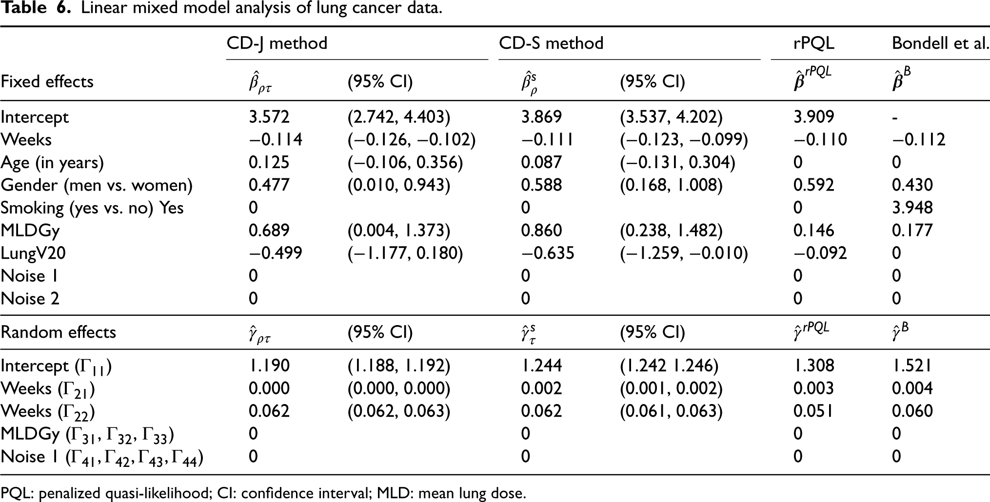
Data with 777 observations from the 111 NSCLC patients were included in the data analysis. The outcome variable, tumor volume, was log-transformed to ensure normality. Potential covariates considered for the fixed effect selection included Weeks (weeks from the start of radiation cycle), Age (age when radiation therapy started), Gender (women vs. men), smoking (yes vs. no), mean lung dose, and Lung V20. Mean lung dose (MLDGy) measured how much radiation dose the normal lung tissues have received, and Lung V20 (LungV20) was the portion of normal lung volume that received 20 Gy of radiation dose. Weeks and MLDGy were considered for the random effect selection. All continuous variables were standardized to have mean 0 and variance 1. In order to evaluate the performance of the proposed methods , we have randomly generated 2 noise variables following standard normal distribution and included them to the fixed effect selection. One of these noise variables was also included in the random effect selection. Results were summarized in Table 6. For the fixed effect selection by the CD-J method, the randomly generated noise variables were not selected. Weeks, Age, Gender, MLDGy, and LungV20 were selected. Specifically, the selected fixed effect estimates suggested that tumor volume decreased with Weeks ( ${\hat{\beta }}_{\rho \tau }=-0.114$ , 95% CI: [ $-0.126,-0.102$ ]), and was larger in men than women ( ${\hat{\beta }}_{\rho \tau }=0.477$ , 95% CI: [ $0.010,0.943$ ]). The mean tumor size also increased with MLDGy ( ${\hat{\beta }}_{\rho \tau }=0.689$ , 95% CI: [ $0.004,1.373$ ]) and decreased with LungV20 ( ${\hat{\beta }}_{\rho \tau }=-0.499$ , 95% CI: [ $-1.177,0.180$ ]). Random intercept ( ${\hat{\mathrm{\Gamma }}}_{11}=1.190$ , 95% CI: [ $1.188,1.192$ ]) and random slope for Weeks ( ${\hat{\mathrm{\Gamma }}}_{21}=0.000$ , 95% CI: [ $0.000,0.000$ ], and ${\hat{\mathrm{\Gamma }}}_{22}=0.062$ , 95% CI: [ $0.062,0.063]$ ) were selected, suggesting a positive within-person correlation and a heterogeneous effect by Weeks. Results from CD-S were similar. We also applied the rPQL and Bondell’s methods to this dataset. Neither of these methods selected the noise variables. The rPQL didn’t select Age in the fixed effect. Bondell’s method did not select Age but selected Smoking. For the random effect selection, all four methods selected the same random effects.

Table 6.

Linear mixed model analysis of lung cancer data.

	CD-J method		CD-S method		rPQL	Bondell et al.
Fixed effects	${\hat{\beta }}_{\rho \tau }$	(95% CI)	${\hat{\beta }}_{\rho }^s$	(95% CI)	${\hat{\mathit{\beta }}}^{rPQL}$	${\hat{\mathit{\beta }}}^B$
Intercept	3.572	(2.742, 4.403)	3.869	(3.537, 4.202)	3.909	-
Weeks	$-$ 0.114	( $-$ 0.126, $-$ 0.102)	$-$ 0.111	( $-$ 0.123, $-$ 0.099)	$-$ 0.110	$-$ 0.112
Age (in years)	0.125	( $-$ 0.106, 0.356)	0.087	( $-$ 0.131, 0.304)	0	0
Gender (men vs. women)	0.477	(0.010, 0.943)	0.588	(0.168, 1.008)	0.592	0.430
Smoking (yes vs. no) Yes	0		0		0	3.948
MLDGy	0.689	(0.004, 1.373)	0.860	(0.238, 1.482)	0.146	0.177
LungV20	$-$ 0.499	( $-$ 1.177, 0.180)	$-$ 0.635	( $-$ 1.259, $-$ 0.010)	$-$ 0.092	0
Noise 1	0		0		0	0
Noise 2	0		0		0	0
Random effects	${\hat{\gamma }}_{\rho \tau }$	(95% CI)	${\hat{\gamma }}_{\tau }^s$	(95% CI)	${\hat{\gamma }}^{rPQL}$	${\hat{\gamma }}^B$
Intercept ( ${\mathrm{\Gamma }}_{11}$ )	1.190	(1.188, 1.192)	1.244	(1.242 1.246)	1.308	1.521
Weeks ( ${\mathrm{\Gamma }}_{21}$ )	0.000	(0.000, 0.000)	0.002	(0.001, 0.002)	0.003	0.004
Weeks ( ${\mathrm{\Gamma }}_{22}$ )	0.062	(0.062, 0.063)	0.062	(0.061, 0.063)	0.051	0.060
MLDGy ( ${\mathrm{\Gamma }}_{31}$ , ${\mathrm{\Gamma }}_{32}$ , ${\mathrm{\Gamma }}_{33}$ )	0		0		0	0
Noise 1 ( ${\mathrm{\Gamma }}_{41},{\mathrm{\Gamma }}_{42},{\mathrm{\Gamma }}_{43},{\mathrm{\Gamma }}_{44}$ )	0		0		0	0

PQL: penalized quasi-likelihood; CI: confidence interval; MLD: mean lung dose.

Data Example 2. Patients with early-stage breast cancer are commonly treated with breast-conserving therapy (BCT), which includes lumpectomy followed by radiation therapy. Prior studies with long-term follow-up have demonstrated equivalent overall survival in those treated with lumpectomy and radiation, compared with those who underwent mastectomy.^42,43 Because mammographic alterations after BCT can mimic or hide tumor recurrence, they become clinically relevant when unnecessary biopsies or delayed diagnoses occur. Then this study longitudinally followed up the mammographic changes in early-stage breast cancer patients after BCT, and is interested in identifying covariates associated with the incidence or changes of common mammographic sequelae. ⁴⁴

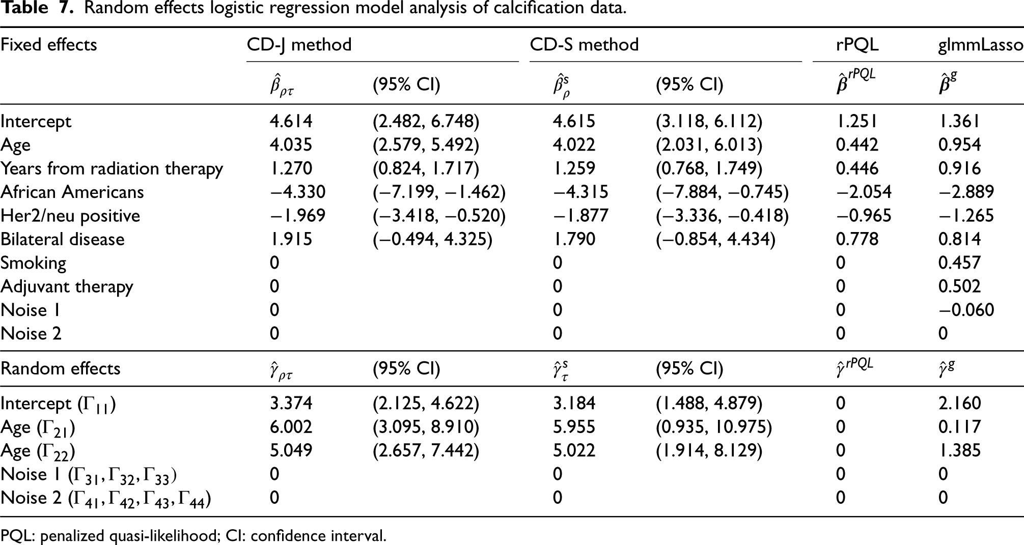
Data from 89 patients with a total of 605 longitudinally measured observations were included in the data analysis. Among several image parameters, we fitted a random effects logistic regression model with calcification (yes vs. no) as the dependent variable, and applied the proposed CD-S method to select fixed effects from the following covariates: age (years), years from radiation therapy, African Americans (yes vs. no), Her2/neu positive (yes vs. no), adjuvant chemo and/or hormonal therapy (yes vs. no), smoking (yes vs. no), bilateral disease (yes vs. no) and 2 unrelated and randomly generated standard normal noise variables. Potential covariates for the random effect selection included the intercept, age, and the two unrelated noise variables that were also included in the fixed effect selection. All continuous variables were standardized to have mean 0 and variance 1. Results were summarized in Table 7. For the fixed effect selection, the randomly generated noise variables were not selected. Age, years since radiation therapy, African Americans, Her2/neu positive, and Bilateral Disease were selected. For instance, estimates of the selected fixed effects suggested that the risk of calcification increased with age ( ${\hat{\beta }}_{\rho \tau }=4.035$ , 95% CI: [ $2.579,5.492$ ]), years since radiation therapy ( ${\hat{\beta }}_{\rho \tau }=1.270$ , 95% CI: [ $0.824,1.717$ ]), and was lower in African Americans ( ${\hat{\beta }}_{\rho \tau }=-4.330$ , 95% CI: [ $-7.199,-1.462$ ]). For random effects, age ( ${\hat{\mathrm{\Gamma }}}_{21}=6.002$ , 95% CI: [ $3.095,8.910$ ], and ${\hat{\mathrm{\Gamma }}}_{22}=5.049$ , 95% CI: [ $2.657,7.442$ ]) was selected, in addition to the random intercept ( ${\hat{\mathrm{\Gamma }}}_{11}=3.374$ , 95% CI: [ $2.125,4.622$ ]), suggesting a positive within-person correlation and a heterogeneous effect by age. Results from the CD-S method were similar. We applied the rPQL and glmmLasso methods to this dataset. Because glmmLasso only performs the fixed effect selection, we only included the intercept and age as random effects in the model and reported the parameter estimates for reference. The rPQL method selected the same fixed effect covariates as the CD-S method, but did not select any random effects. The method of glmmLasso selected more fixed effect covariates. The magnitude of the selected fixed effect coefficient estimates of these two methods were generally smaller than that by the CD methods, consistent with the observations from the simulation studies.

Table 7.

Random effects logistic regression model analysis of calcification data.

Fixed effects	CD-J method		CD-S method		rPQL	glmmLasso
	${\hat{\beta }}_{\rho \tau }$	(95% CI)	${\hat{\beta }}_{\rho }^s$	(95% CI)	${\hat{\mathit{\beta }}}^{rPQL}$	${\hat{\mathit{\beta }}}^g$
Intercept	4.614	(2.482, 6.748)	4.615	(3.118, 6.112)	1.251	1.361
Age	4.035	(2.579, 5.492)	4.022	(2.031, 6.013)	0.442	0.954
Years from radiation therapy	1.270	(0.824, 1.717)	1.259	(0.768, 1.749)	0.446	0.916
African Americans	$-$ 4.330	( $-$ 7.199, $-$ 1.462)	$-$ 4.315	( $-$ 7.884, $-$ 0.745)	$-$ 2.054	$-$ 2.889
Her2/neu positive	$-$ 1.969	( $-$ 3.418, $-$ 0.520)	$-$ 1.877	( $-$ 3.336, $-$ 0.418)	$-$ 0.965	$-$ 1.265
Bilateral disease	1.915	( $-$ 0.494, 4.325)	1.790	( $-$ 0.854, 4.434)	0.778	0.814
Smoking	0		0		0	0.457
Adjuvant therapy	0		0		0	0.502
Noise 1	0		0		0	$-$ 0.060
Noise 2	0		0		0	0
Random effects	${\hat{\gamma }}_{\rho \tau }$	(95% CI)	${\hat{\gamma }}_{\tau }^s$	(95% CI)	${\hat{\gamma }}^{rPQL}$	${\hat{\gamma }}^g$
Intercept ( ${\mathrm{\Gamma }}_{11}$ )	3.374	(2.125, 4.622)	3.184	(1.488, 4.879)	0	2.160
Age ( ${\mathrm{\Gamma }}_{21}$ )	6.002	(3.095, 8.910)	5.955	(0.935, 10.975)	0	0.117
Age ( ${\mathrm{\Gamma }}_{22}$ )	5.049	(2.657, 7.442)	5.022	(1.914, 8.129)	0	1.385
Noise 1 ( ${\mathrm{\Gamma }}_{31},{\mathrm{\Gamma }}_{32},{\mathrm{\Gamma }}_{33})$	0		0		0	0
Noise 2 ( ${\mathrm{\Gamma }}_{41},{\mathrm{\Gamma }}_{42},{\mathrm{\Gamma }}_{43},{\mathrm{\Gamma }}_{44}$ )	0		0		0	0

PQL: penalized quasi-likelihood; CI: confidence interval.

7. Discussion

In this paper, we propose a regularized estimation approach using the confidence distributions of model parameters to select both fixed and random effects in GLMMs. Specifically, we propose to construct and optimize the objective functions based on the confidence distributions of model parameters, as opposed to the objective functions typically constructed from the likelihood function using the observed data. This can greatly alleviate the computational burden in approximating the integral in the log marginal likelihood function in the regularization step.

We started from showing that the log marginal likelihood function, after integrating out the random effects, can be approximated by the log confidence density of the model parameters based on the asymptotic distribution of the MLEs. As a result, we propose the CD-joint estimation method by constructing the objective functions using the confidence density, as opposed to the observed data likelihood function. Because the joint confidence density of the fixed effect and random effect parameters is a multivariate normal density, the parameters of the joint distribution and the marginal distribution are the same. Therefore, we propose the CD-separate estimation method by constructing the objective functions based on the marginal confidence density corresponding to the fixed effect and random effect parameters, respectively. In spite that the CD-joint estimators and CD-separate estimators are different estimators, the true values of the underlying parameters of these estimators are the same. With a proper choice of regularization parameters in the adaptive LASSO framework, we show that the proposed estimators have consistency and oracle properties. Based on the asymptotic properties of the proposed estimators and our simulation studies, when the sample size (i.e. the number of independent cluster, $n$ ) is large, our methods generally performed well and do not require to refit a GLMM model after the variable selection step. However, when $n$ is small, we noticed that our methods may result in bigger bias and false selection rate (e.g. $n=30$ and $m=10$ in the simulation studies of random effect logistic regression analysis). Thus, similar to Hui et al., ¹⁹ we recommend the hybrid estimation approach, e.g. refitting a GLMM model using REML after the variable selection step, to improve the finite sample performance. Moreover, because GLMM typically requires the assumption that the random effects follow a multivariate normal distribution with mean 0, we applied this assumption in our simulation studies to assess the performance of the proposed methods. In case this assumption is violated and the random effects are following a right-skewed distribution with non-zero means, it is likely to cause biased GLMM estimates and affect the asymptotic distributions of the estimators. Because the proposed CD methods are built upon the asymptotic distributions of the GLMM estimators, we expect the performance of our methods will be negatively affected due to the deviation from this assumption.

The proposed CD methods require obtaining the GLMM estimates in order to apply the confidence distribution approach and perform the variable selections, while other methods, e.g. the Bondell’s ⁶ method, may not require this condition, and some may only need good initial estimates to implement their methods, e.g. the rPQL ¹⁹ method. To implement our methods in practice, one may construct the proposed objective functions by using existing software packages (e.g. lme4 package in R and Proc Glimmix in SAS) that provide readily available solutions of $\hat{\mathit{\theta }}$ and $\hat{\mathbf{\Sigma }}$ . Then optimizing the proposed objective functions to obtain the regularized estimators no longer involves the numerical approximation of the integral in the log marginal likelihood function, and thus boosts computational efficiency. Moreover, optimizing the proposed objective functions in the regularized estimation process can also use existing software packages without the need to develop new computational algorithms specific to GLMM.

When the data are independent, the proposed CD-J method generally does not work due to the singularity of the joint variance-covariance of the fixed and random effect parameter estimates. For the proposed CD-S method, the fixed effect selection still works well, but the random effect selection does not, due to the same singularity issue of the variance-covariance of the random effect estimates. Therefore, we recommend to apply our methods when the dependent variables are correlated and the GLMM analysis can produce meaningful random effect estimates.

Due to the asymptotic normality property of the MLE, we notice that the proposed CD-based objective functions take the similar forms to the objective function based on the LSA proposed by Wang and Leng ³² for the generalized linear models. Simulation studies demonstrate the consistency, oracle properties and computational efficiency, especially when the number of independent clusters $n$ is large. The coverage probability of the 95% CI seemed to be lower than the nominal 95% level in some cases. Replacing $\hat{\mathbf{\Sigma }}$ by other consistent estimators of $\mathrm{\Sigma }$ , for instance, the robust sandwich variance estimator^45,46 might improve the coverage probability.

For future work, we will extend our method to the framework of generalized estimating equation approach ⁴⁷ for correlated outcome data. The extension to other likelihood-based approaches for complex modeling, such as the joint analysis of survival and longitudinal data analysis, will also be explored.

Supplemental Material

sj-pdf-1-smm-10.1177_09622802231221201 - Supplemental material for Fixed and random effect selections in generalized linear mixed models

Supplemental material, sj-pdf-1-smm-10.1177_09622802231221201 for Fixed and random effect selections in generalized linear mixed models by Shou-En Lu, Sinae Kim, Jerry Q Cheng, Changfa Lin, Sharad Goyal and Salma K Jabbour in Statistical Methods in Medical Research