Confidence estimation based on data from independent studies

Abstract

The problem of finding confidence intervals based on data from several independent studies or experiments is considered. A general method of finding confidence intervals by inverting a combined test is proposed. The combined tests considered are the Fisher test, the weighted inverse normal test, the inverse chi-square test and the inverse Cauchy test. The method is illustrated for finding confidence intervals for a common mean of several normal populations, common correlation coefficient of several bivariate normal populations, common coefficient of variation, common mean of several lognormal populations, and for a common mean of several gamma populations. For each case, the confidence intervals based on the combined tests are compared with the other available approximate confidence intervals with respect to coverage probability and precision. R functions to compute all confidence intervals are provided in a supplementary file. The methods are illustrated using several practical examples.

1. Introduction

There are many areas of the medical, behavioral, and social sciences where we have data or summary results available from several independent studies, experiments, or laboratories all addressing the same objective. Major medical hypotheses are typically studied more than once, often by different clinical research teams in different locations. Analysis of results from different sources or results of earlier research to derive conclusions about the body of research is known as meta-analysis. Usually, the study is based on randomized, controlled clinical trials. Such problems also arise, for example, when two or more independent agencies are involved in estimating the effect of a new drug, when several measuring instruments are used to measure the products produced by the same production process to assess the average quality, or when different laboratories are used to measure the amount of toxic waste in a river. There is a need to combine the results from independent sources or experiments to make inference on the common objective of interest. Egger and Smith ¹ have noted that “A single study often cannot detect or exclude with certainty a modest, albeit clinically relevant, difference in the effects of two treatments. A trial may thus show no significant treatment effect when in reality such an effect exists.” Regarding multivariate meta-analysis, Jackson et al. ² have noted that effects are often multivariate rather than univariate and medical studies often examine multiple, and correlated, outcomes of interest to the meta-analyst.

In this article, we address the problem of testing and interval estimating a common parameter of interest based on independent data sets collected from different sources. Common parameters could be the mean of several populations, coefficient of variation (CV) of several measurements obtained using different instruments, common coefficient of correlation of several bivariate normal populations, and so on. Examples with data or summary statistics for testing/estimating a common mean of several populations are given in many articles. Meier ³ has provided an example where data collected from four experiments that were used to estimate the mean percentage of albumin in the plasma protein of normal human subjects. Eberhardt et al. ⁴ provided three examples each of which is concerned with estimating a chemical substance in non-fat milk powder by combining the results of different analytical methods. Skinner ⁵ presented examples related to clinical trials and determining the density of nitrogen using different laboratory methods. In these situations, the variances are typically unequal due to the variation in different methods or measuring instruments and the objective is to estimate the common mean of measurements from different sources. These authors have provided solutions assuming normal models with the same mean but possibly different variances. The common mean problem has also been addressed assuming lognormal distributions (e.g. Tian and Wu ⁶ and Krishnamoorthy and Oral ⁷ ), and gamma distributions. ⁸

Another common parameter of several populations that is of interest is the CV, which is a commonly used measure of variability in experimental studies. Smaller values of CV indicate higher precision of measurements or of the experimental results. The CV is a preferred measure of variability because, unlike the variance, it does not depend on units of measurement. If it is reasonable to assume that a common CV in various independent experimental results, then it is of interest to test or interval estimate the common CV. Tian ⁹ and Forkman ¹⁰ have considered the problem of estimating the common CV of several normal populations. This seems to be an important problem with applications as Tian’s research was attracted by many researchers and practitioners. Both papers present some approximate confidence intervals for the common CV of several normal populations.

Combining the results from independent sources for estimating a common correlation coefficient of several bivariate normal populations has received considerable attention in the literature; see Donner and Rosner, ¹¹ Tian and Wilding ¹² and Liu and Xu. ¹³ Donner and Rosner have proposed an approximate interval estimation method based on a linear function of independent Fisher $Z$ statistics. Tian and Wilding ¹² have described a generalized variable (GV) approach to find a confidence interval (CI) for a common correlation coefficient and Liu and Xu ¹³ have proposed a solution for the problem based on confidence distribution.

In general, if independent tests were carried out in different locations for a common purpose of interest, then a popular method of combining the test results is Fisher’s ¹⁴ method of combining $p$ -values of the independent tests to arrive at a single test; see Mathew et al. ¹⁵ and the references therein. Fisher’s combination of $p$ -values has a chi-square distribution, and so it is easy to determine the $p$ -value or critical region of the combined test. Stouffer et al. ¹⁶ proposed an alternative combined test that is based on independent normal $z$ -scores. Liptak ¹⁷ has suggested to use a weighted average of the $z$ -scores. Folks ¹⁸ and other authors have found that Fisher’s test performed well over a wide range of parameter values and that the Liptak-Stouffer inverse-normal method performed poorly. However, for the normal case, Whitlock ¹⁹ has noted that the Liptak-Stouffer test with weights proportional to the degrees of freedom (df) is better than the Fisher test. Liu and Xie ²⁰ proposed Cauchy combination test that combines independent $p$ -values using inverse of Cauchy distributions. This Cauchy combined test tackles some dependency structures of the proposed test statistic in their paper. ²⁰ Recently, Krishnamoorthy et al. ²¹ have considered a new test based on chi-square scores and compared several combined tests for a common mean of normal populations, common correlation coefficient, common CV and for a common mean of several lognormal populations. On the basis of extensive simulation study, they found that no test is uniformly better than the other tests for all problems. For some specific problems, they noted that some tests perform better than others over a wide range of parameter space.

Even though there are several papers that have addressed the testing problems of combining independent tests for various purposes, only a few papers considered the problems of interval estimating a common parameter of interest in various setups. For estimating a common mean of several normal populations, Fairweather ²² and Jordan and Krishnamoorthy ²³ have provided CIs based on pivotal-based approaches. Tian and her co-authors have proposed CIs for a common correlation coefficient, a common CV and a common mean of several lognormal populations; see Tian, ⁹ Tian and Wilding ¹² and Tian and Wu. ⁶ These authors have proposed approximate CIs based on the GV approach by Weerahandi. ²⁴ Donner and Rosner ¹¹ have developed an approximate CI for a common correlation coefficient of several bivariate normal populations on the basis of a combination of Fisher’s $z$ -statistics.

Most of the CIs proposed in the literature are approximate and not simple to compute. Our point here is that even though all available combined tests are exact in the frequentist sense, CIs that can be obtained by inverting the exact combined tests are not proposed in the literature. The purpose of this article is to describe interval estimation procedures based on several combined tests and make them readily available to researchers and practitioners of statistics. We propose a numerical approach to find a CI for a common parameter of interest by inverting a combined test and illustrate the procedure for several problems. In the following section, we describe a numerical approach to find a CI for a common parameter of interest by inverting a combined test. The method is applied to find confidence intervals for (a) a common mean of several normal populations (Section 3), (b) a common CV (Section 4), (c) a common mean of several lognormal populations (Section 5), (d) a common correlation coefficient of several bivariate normal populations (Section 6, (e) a common mean of several gamma populations (Section 7). For each problem, we considered CIs based on Fisher’s combined test, weighted inverse normal test (Liptak-Stouffer test), inverse Cauchy test ²⁰ and inverse ${\chi }^2$ test. Furthermore, CIs based on these combined tests are also compared with other available approximate CIs in terms of coverage probability and precision. An illustrative example with real data are given for each of the estimation problems. To help practitioners compute these CIs, we provide R functions in a supplementary file. Some concluding remarks are given in Section 8. R functions to compute CIs using the Fisher, weighted inverse normal, inverse Cauchy, and inverse chi-square are provided in a supplementary file.

2. Confidence intervals from combined tests

Suppose that there are $k$ independent populations with a common parametric function of interest. Let us denote the common parametric function by $\xi =\xi ({\theta }_{11},\dots ,{\theta }_{l1})=\cdots =\xi ({\theta }_{1k},\dots ,{\theta }_{lk})$ , where $\xi$ is a known function and ${\theta }_{ij}$ , $i=1,\dots ,l$ , $j=1,\dots ,k$ , are unknown parameters. Assume that a sample of size $n_i$ is available from the $i$ th population, $i=1,\dots ,k$ . Assume also that the samples are independent. Consider testing

$$H_0:\xi \le {\xi }_0\mathrm{vs}.H_a:\xi >{\xi }_0,$$

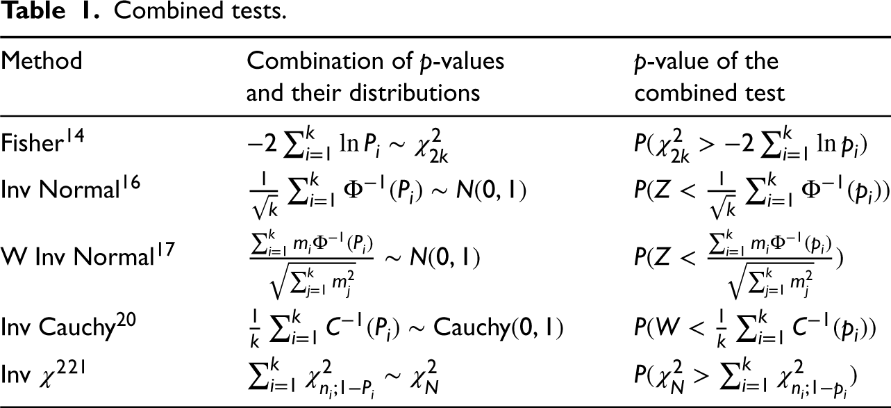
(1) where ${\xi }_0$ is a specified value. Let $P_i$ denote the $p$ -value of a test for the above hypotheses based on the $i$ th sample, $i=1,\dots ,k$ . The $p$ -values are based on independent samples, so they are independent uniform $(0,1)$ random variables. To arrive at a combined test based on all samples, some transformed $p$ -values are combined to obtain a single test statistic so that its null distribution does not depend on any unknown parameter. In Table 1, we provide some well-known combined tests, namely, Fisher’s test, inverse normal test, weighted inverse normal test, inverse Cauchy test and the inverse ${\chi }^2$ test. The notations used in the table are as follows:

• $\mathrm{\Phi }=$ standard normal distribution function

• $Z=$ standard normal random variable

• $N=\sum _{i=1}^k{n}_i$ and $m_i=n_i-1$ , $i=1,\dots ,k.$

• $P_i$ is the $p$ -value based on the $i$ th sample, $i=1,\dots ,k$ .

• $(p_1,\dots ,p_k)$ is an observed value of $(P_1,\dots ,P_k)$

• $W=$ the standard Cauchy random variable with the distribution function $C(x)$

• ${\chi }_{m;\alpha }^2=$ the 100 $\alpha$ percentile of the chi-squared distribution with df = $m$ .

Table 1.

Combined tests.

Method	Combination of $p$ -values	$p$ -value of the
	and their distributions	combined test
Fisher 14	$-2\sum _{i=1}^k\ln P_i\sim {\chi }_{2k}^2$	$P({\chi }_{2k}^2>-2\sum _{i=1}^k\ln p_i)$
Inv Normal 16	$\frac{1}{\sqrt{k}}\sum _{i=1}^k{\mathrm{\Phi }}^{-1}(P_i)\sim N(0,1)$	$P(Z<\frac{1}{\sqrt{k}}\sum _{i=1}^k{\mathrm{\Phi }}^{-1}(p_i))$
W Inv Normal 17	$\frac{\sum _{i=1}^k{m}_i{\mathrm{\Phi }}^{-1}(P_i)}{\sqrt{\sum _{j=1}^k{m}_j^2}}\sim N(0,1)$	$P(Z<\frac{\sum _{i=1}^k{m}_i{\mathrm{\Phi }}^{-1}(p_i)}{\sqrt{\sum _{j=1}^k{m}_j^2}})$
Inv Cauchy 20	$\frac{1}{k}\sum _{i=1}^k{C}^{-1}(P_i)\sim \mathrm{Cauchy}(0,1)$	$P(W<\frac{1}{k}\sum _{i=1}^k{C}^{-1}(p_i))$
Inv ${\chi }^2$ 21	$\sum _{i=1}^k{\chi }_{n_i;1-P_i}^2\sim {\chi }_N^2$	$P({\chi }_N^2>\sum _{i=1}^k{\chi }_{n_i;1-p_i}^2)$

At the level $\alpha$ , a combined test rejects the null hypothesis $H_0:\xi \le {\xi }_0$ in favor of the alternative hypothesis $H_a:\xi >{\xi }_0$ if the $p$ -value is less than $\alpha$ . The value $L$ of ${\xi }_0$ for which the $p$ -value of a combined test is equal to $\alpha$ is a $1-\alpha$ lower confidence limit for $\xi$ . Similarly, by inverting a combined test for $H_0:\xi \ge {\xi }_0$ vs. $H_a:\xi <{\xi }_0$ , we can find a $1-\alpha$ upper confidence limit $U$ for $\xi$ . The interval $(L,U)$ is a $1-2\alpha$ two-sided CI for $\xi$ .

In general, a CI from a combined test can be obtained only by numerically. The following algorithm may be used to find a CI for a common parameter by inverting the Fisher combined test. Confidence intervals based on other combined tests can be obtained similarly.

Algorithm 1

1. (1)

Compute the $p$ -values $P_i({\xi }_0)$ ’s for testing $H_0:\xi \le {\xi }_0$ vs. $H_a:\xi >{\xi }_0$ based on the sample of size $n_i$ from the $i$ th population, $i=1,\dots ,k$ .

(2)

Compute the combined statistic $-2\sum _{i=1}^k\ln P_i({\xi }_0)$ .

(3)

Set the function $f({\xi }_0)=P({\chi }_{2k}^2>-2\sum _{i=1}^k\ln P_i({\xi }_0))$ .

(4)

Solve $f({\xi }_0)-\alpha =0$ for ${\xi }_0$ .

(5)

The root of the equation in the preceding step is a $1-\alpha$ lower confidence limit for $\xi$ .

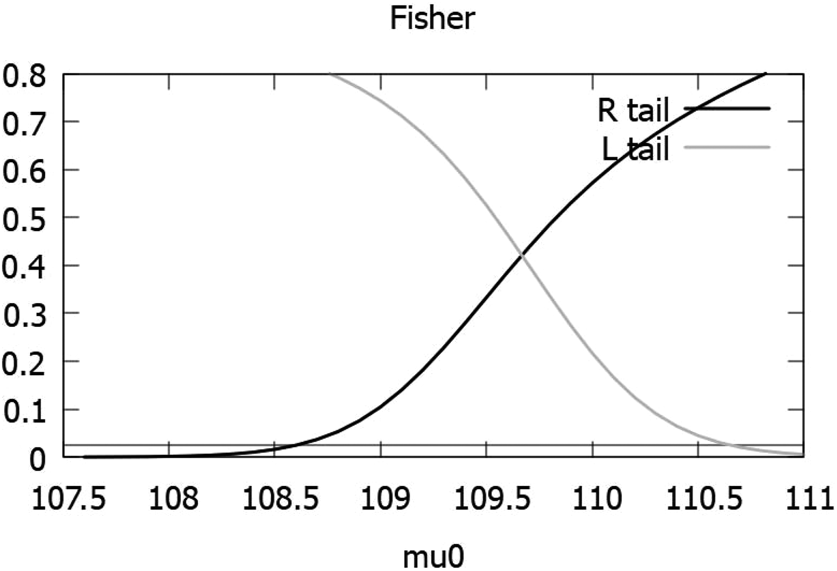
To compute an upper confidence limit for $\xi$ , we use the $p$ -values $P_i({\xi }_0)$ ’s for testing $H_0:\xi \ge {\xi }_0$ vs. $H_a:\xi <{\xi }_0$ in Step 1 and then follow Steps 2 – 5. The $100(1-\alpha )$ % one-sided confidence limits form a 100 $(1-2\alpha )$ % two-sided CI for the parameter $\xi$ . For a graphical illustration of Algorithm 1 for finding CIs for a common mean of several normal distributions, see Figure 1.

Figure 1.

$P$ -values of the Fisher test as a function of ${\mu }_0$ for the data in Table 3; the horizontal line is $y=0.025$ line.

3. Common mean of several normal distributions

Let $({\overline{X}}_i,S_i^2)$ denote the (mean, variance) based on a sample of size $n_i$ from a $N(\mu ,{\sigma }_i^2)$ distribution, $i=1,\dots ,k$ . The variance $S_i^2$ is defined with the divisor $m_i=n_i-1$ , $i=1,\dots ,k.$

3.1. Confidence intervals

We first describe some available exact and approximate CIs for a common mean of several normal populations.

3.1.1. Confidence interval based on a weighted F statistics

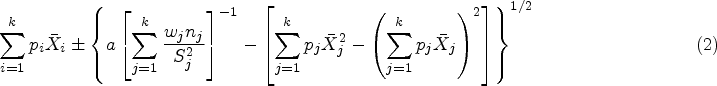
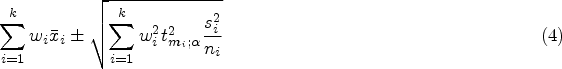
Jordan and Krishnamoorthy ²³ have proposed a CI by inverting a linear combination of $F$ -test statistics for the normal mean $\mu .$ To describe this CI, let $F_i$ denote the $F$ random variable with 1 and $m_i$ degrees of freedoms, and let $a$ denote the 100 $(1-\alpha )$ percentile of $\sum _{i=1}^k{w}_i{F}_i$ . Let $w_i=[\mathrm{Var}{F}_i{]}^{-1}/[\sum _{j=1}^k[\mathrm{Var}{F}_j{]}^{-1}]$ and $p_i=(w_i{n}_i/S_i^2)/[\sum _{j=1}^k{w}_j{n}_j/S_j^2].$ Then

$$\sum _{i=1}^k{p}_i{\overline{X}}_i\pm {\{a{\left[\sum _{j=1}^k\frac{w_j{n}_j}{S_j^2}\right]}^{-1}-[\sum _{j=1}^k{p}_j{\overline{X}}_j^2-{\left(\sum _{j=1}^k{p}_j{\overline{X}}_j\right)}^2]\}}^{1/2}$$

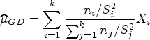
(2) is an exact $(1-\alpha )$ CI for $\mu$ . The above CI is centered at the Graybill-Deal ²⁵ estimator

$${\hat{\mu }}_{GD}=\sum _{i=1}^k\frac{n_i/S_i^2}{\sum _{j=1}^k{n}_j/S_j^2}{\overline{X}}_i$$

of $\mu$ if $w_i=1$ for all $i$ . For $k\ge 2$ , the percentile $a$ can also be estimated using Monte Carlo simulation or approximated using the method in Jordan and Krishnamoorthy. ²³ Since the variance of $F_i$ which is defined when the df $m_i\ge 5$ or equivalently, $n_i\ge 6$ for $i=1,\dots ,k$ , the above CI is defined only when all sample sizes are at least 6.

3.1.2. Fiducial confidence intervals

Let $({\overline{x}}_i,s_i^2)$ be an observed value of $({\overline{X}}_i,S_i^2)$ , $i=1,\dots ,k$ . The fiducial variable for $\mu$ based on the $i$ th sample is given by $Q_{i,\mu }={\overline{x}}_i+t_{m_i}\frac{s_i}{\sqrt{n_i}},i=1,\dots ,k,$ where $t_{m_i}$ ’s are independent $t$ random variables with df $m_i$ ; see Section 2.1 of Krishnamoorthy and Mathew. ²⁶ Let $w_i=\frac{n_i}{s_i^2}/\sum _{j=1}^k\frac{n_j}{s_j^2}$ so that $\sum _{i=1}^k{w}_i=1.$ A combined fiducial variable for $\mu$ is given by

$$Q_{\mu }=\sum _{i=1}^k{w}_i{Q}_{i,\mu }=\sum _{i=1}^k{w}_i{\overline{x}}_i+\sum _{i=1}^k{w}_i\frac{s_i}{\sqrt{n_i}}{t}_{m_i}$$

(3) For a given set of statistics $({\overline{x}}_1,s_1),\dots ,({\overline{x}}_k,s_k)$ , the lower and upper 100 $\alpha$ percentiles of $Q_{\mu }$ form a $1-2\alpha$ fiducial CI for $\mu$ . To find this fiducial CI, we need to find the percentiles of $T=\sum _{i=1}^k{w}_i\frac{s_i}{\sqrt{n_i}}{t}_{m_i}$ , which can be estimated using Monte Carlo simulation. The percentiles of $T$ can also be approximated using the normal-based approximation ²⁷ as $T_{\alpha }\simeq \sqrt{\sum _{i=1}^k{w}_i^2{t}_{m_i;\alpha }^2\frac{s_i^2}{n_i}},$ where $t_{m;\alpha }$ is the $\alpha$ quantile of the $t$ distribution with df = $m$ . Using these approximate percentiles, a $1-2\alpha$ fiducial CI for $\mu$ can be expressed as

$$\sum _{i=1}^k{w}_i{\overline{x}}_i\pm \sqrt{\sum _{i=1}^k{w}_i^2{t}_{m_i;\alpha }^2\frac{s_i^2}{n_i}}$$

(4) It can be readily verified that the above CI simplifies to the usual $t$ interval when $k=1$ .

Remark 1. Krishnamoorthy and Lu ²⁸ have proposed a generalized CI for a common mean. Their CI is essentially based the fiducial approach and not in closed-form. It requires Monte Carlo simulation to estimate whereas the CI in (4) is simple and it requires only $t$ percentiles to compute.

3.1.3. Confidence intervals based on a combined test

To deduce a CI from a combined test given in Table 1, consider testing $H_0:\mu ={\mu }_0$ vs. $H_a:\mu >{\mu }_0$ , where $\mu$ is a common mean of $k$ independent normal populations. The $p$ -value of the usual $t$ -test based on the $i$ th sample is given by $P_i=P(t_{m_i}>\sqrt{n_i}({\overline{X}}_i-{\mu }_0)/S_i)$ , where $t_{m_i}$ denotes the $t$ random variable with df $m_i=n_i-1$ , $i=1,\dots ,k$ . Using these independent $p$ -values in any of the combined tests in Table 1 and Algorithm 1, a lower confidence limit for the common mean $\mu$ can be computed. Similarly, by inverting a left-tailed combined test, an upper confidence limit for $\mu$ can be obtained.

3.2. Normal: Coverage and precision studies

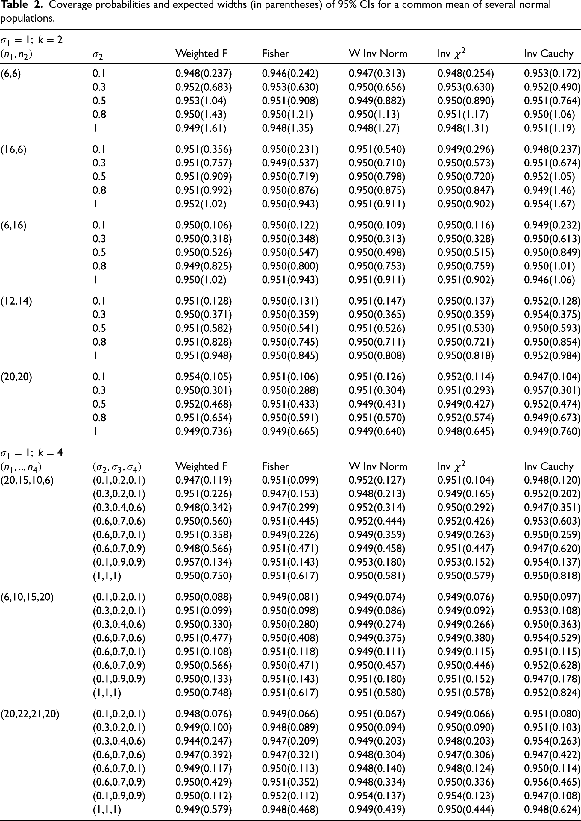
The individual $t$ tests based on independent samples are exact and so do the combined tests. Therefore, the CIs based on any combined test in Table 1 are exact. To compare the CIs based on combined tests in terms of precision and to judge the accuracy of the approximate fiducial CIs and the CIs based on the weighted $F$ statistics, we estimated the coverage probabilities and expected widths of all CIs and reported them in Table 2. Monte Carlo estimates of the coverage probabilities and expected widths are based on 10,000 simulations runs. These estimates were obtained for the case of $k=2$ and 4. The CIs based on the inverse normal combined test and approximate fiducial method are not included in the simulation study because our preliminary study (not reported here) indicated that the inverse normal combined test is inferior to those based on the weighted inverse normal test. Furthermore, the closed-form approximate fiducial CIs are liberal when sample sizes are small. They are satisfactory in terms of coverage and precision if all sample sizes are 30 or more. For such sample sizes, the approximate fiducial CIs are satisfactory in terms of coverage probability and are expected to be slightly shorter than the other CIs.

Table 2.

Coverage probabilities and expected widths (in parentheses) of 95% CIs for a common mean of several normal populations.

${\sigma }_1=1;k=2$
$(n_1,n_2)$	${\sigma }_2$	Weighted F	Fisher	W Inv Norm	Inv ${\chi }^2$	Inv Cauchy
(6,6)	0.1	0.948(0.237)	0.946(0.242)	0.947(0.313)	0.948(0.254)	0.953(0.172)
	0.3	0.952(0.683)	0.953(0.630)	0.950(0.656)	0.953(0.630)	0.952(0.490)
	0.5	0.953(1.04)	0.951(0.908)	0.949(0.882)	0.950(0.890)	0.951(0.764)
	0.8	0.950(1.43)	0.950(1.21)	0.950(1.13)	0.951(1.17)	0.950(1.06)
	1	0.949(1.61)	0.948(1.35)	0.948(1.27)	0.948(1.31)	0.951(1.19)
(16,6)	0.1	0.951(0.356)	0.950(0.231)	0.951(0.540)	0.949(0.296)	0.948(0.237)
	0.3	0.951(0.757)	0.949(0.537)	0.950(0.710)	0.950(0.573)	0.951(0.674)
	0.5	0.951(0.909)	0.950(0.719)	0.950(0.798)	0.950(0.720)	0.952(1.05)
	0.8	0.951(0.992)	0.950(0.876)	0.950(0.875)	0.950(0.847)	0.949(1.46)
	1	0.952(1.02)	0.950(0.943)	0.951(0.911)	0.950(0.902)	0.954(1.67)
(6,16)	0.1	0.950(0.106)	0.950(0.122)	0.950(0.109)	0.950(0.116)	0.949(0.232)
	0.3	0.950(0.318)	0.950(0.348)	0.950(0.313)	0.950(0.328)	0.950(0.613)
	0.5	0.950(0.526)	0.950(0.547)	0.950(0.498)	0.950(0.515)	0.950(0.849)
	0.8	0.949(0.825)	0.950(0.800)	0.950(0.753)	0.950(0.759)	0.950(1.01)
	1	0.950(1.02)	0.951(0.943)	0.951(0.911)	0.951(0.902)	0.946(1.06)
(12,14)	0.1	0.951(0.128)	0.950(0.131)	0.951(0.147)	0.950(0.137)	0.952(0.128)
	0.3	0.950(0.371)	0.950(0.359)	0.950(0.365)	0.950(0.359)	0.954(0.375)
	0.5	0.951(0.582)	0.950(0.541)	0.951(0.526)	0.951(0.530)	0.950(0.593)
	0.8	0.951(0.828)	0.950(0.745)	0.950(0.711)	0.950(0.721)	0.950(0.854)
	1	0.951(0.948)	0.950(0.845)	0.950(0.808)	0.950(0.818)	0.952(0.984)
(20,20)	0.1	0.954(0.105)	0.951(0.106)	0.951(0.126)	0.952(0.114)	0.947(0.104)
	0.3	0.950(0.301)	0.950(0.288)	0.951(0.304)	0.951(0.293)	0.957(0.301)
	0.5	0.952(0.468)	0.951(0.433)	0.949(0.431)	0.949(0.427)	0.952(0.474)
	0.8	0.951(0.654)	0.950(0.591)	0.951(0.570)	0.952(0.574)	0.949(0.673)
	1	0.949(0.736)	0.949(0.665)	0.949(0.640)	0.948(0.645)	0.949(0.760)
${\sigma }_1=1;k=4$
$(n_1,..,n_4)$	$({\sigma }_2,{\sigma }_3,{\sigma }_4)$	Weighted F	Fisher	W Inv Norm	Inv ${\chi }^2$	Inv Cauchy
(20,15,10,6)	(0.1,0.2,0.1)	0.947(0.119)	0.951(0.099)	0.952(0.127)	0.951(0.104)	0.948(0.120)
	(0.3,0.2,0.1)	0.951(0.226)	0.947(0.153)	0.948(0.213)	0.949(0.165)	0.952(0.202)
	(0.3,0.4,0.6)	0.948(0.342)	0.947(0.299)	0.952(0.314)	0.950(0.292)	0.947(0.351)
	(0.6,0.7,0.6)	0.950(0.560)	0.951(0.445)	0.952(0.444)	0.952(0.426)	0.953(0.603)
	(0.6,0.7,0.1)	0.951(0.358)	0.949(0.226)	0.949(0.359)	0.949(0.263)	0.950(0.259)
	(0.6,0.7,0.9)	0.948(0.566)	0.951(0.471)	0.949(0.458)	0.951(0.447)	0.947(0.620)
	(0.1,0.9,0.9)	0.957(0.134)	0.951(0.143)	0.953(0.180)	0.953(0.152)	0.954(0.137)
	(1,1,1)	0.950(0.750)	0.951(0.617)	0.950(0.581)	0.950(0.579)	0.950(0.818)
(6,10,15,20)	(0.1,0.2,0.1)	0.950(0.088)	0.949(0.081)	0.949(0.074)	0.949(0.076)	0.950(0.097)
	(0.3,0.2,0.1)	0.951(0.099)	0.950(0.098)	0.949(0.086)	0.949(0.092)	0.953(0.108)
	(0.3,0.4,0.6)	0.950(0.330)	0.950(0.280)	0.949(0.274)	0.949(0.266)	0.950(0.363)
	(0.6,0.7,0.6)	0.951(0.477)	0.950(0.408)	0.949(0.375)	0.949(0.380)	0.954(0.529)
	(0.6,0.7,0.1)	0.951(0.108)	0.951(0.118)	0.949(0.111)	0.949(0.115)	0.951(0.115)
	(0.6,0.7,0.9)	0.950(0.566)	0.950(0.471)	0.950(0.457)	0.950(0.446)	0.952(0.628)
	(0.1,0.9,0.9)	0.950(0.133)	0.951(0.143)	0.951(0.180)	0.951(0.152)	0.947(0.178)
	(1,1,1)	0.950(0.748)	0.951(0.617)	0.951(0.580)	0.951(0.578)	0.952(0.824)
(20,22,21,20)	(0.1,0.2,0.1)	0.948(0.076)	0.949(0.066)	0.951(0.067)	0.949(0.066)	0.951(0.080)
	(0.3,0.2,0.1)	0.949(0.100)	0.948(0.089)	0.950(0.094)	0.950(0.090)	0.951(0.103)
	(0.3,0.4,0.6)	0.944(0.247)	0.947(0.209)	0.949(0.203)	0.948(0.203)	0.954(0.263)
	(0.6,0.7,0.6)	0.947(0.392)	0.947(0.321)	0.948(0.304)	0.947(0.306)	0.947(0.422)
	(0.6,0.7,0.1)	0.949(0.117)	0.950(0.113)	0.948(0.140)	0.948(0.124)	0.950(0.114)
	(0.6,0.7,0.9)	0.950(0.429)	0.951(0.352)	0.948(0.334)	0.950(0.336)	0.956(0.465)
	(0.1,0.9,0.9)	0.950(0.112)	0.952(0.112)	0.954(0.137)	0.954(0.123)	0.947(0.108)
	(1,1,1)	0.949(0.579)	0.948(0.468)	0.949(0.439)	0.950(0.444)	0.948(0.624)

Table 3.

Selenium content in non-fat milk powder using four methods.

Methods	Sample size	Mean	Variance
1. Atomic absorption Spectrometry	8	105.00	85.711
2. Neutron activation: Instrumental	12	109.75	20.748
3. Neutron activation: Radiochemical	14	109.50	2.729
4. Isotope dilution mass spectrometry	8	113.25	33.640

We observe from the reported results in Table 2 that the CIs based on the weighted $F$ statistics control the coverage probabilities very close to the nominal level for all cases. However, the expected widths of these CIs are larger than those based on combined tests. Comparisons of other CIs based on the Fisher, weighted inverse normal, inverse Cauchy, and inverse ${\chi }^2$ combined tests indicate that there is no clear-cut winner among them. For example, the CIs based on the inverse ${\chi }^2$ test and the weighted inverse normal tests are comparable and they are better than those based on the Fisher test in most cases. However, there are cases where the CIs based on the Fisher test are better than those based on the inverse ${\chi }^2$ test. See the results for $(n_1,n_2)=(16,6)$ and $({\sigma }_1,{\sigma }_2)=(1,.1)$ and $(n_1,\dots ,n_4)=(20,15,10,6)$ and $({\sigma }_1,\dots ,{\sigma }_4)=(1,.6,.7,.1)$ . Similarly, we see that the CIs based on the weighted inverse normal are slightly better than those based on the inverse ${\chi }^2$ test. For example, see the results for $(n_1,\dots ,n_4)=(6,6,6,6)$ and $({\sigma }_1,\dots ,{\sigma }_4)=(1,.6,.7,.6)$ and (1,.6,.7,.9). The inverse Cauchy CIs are, in general, wider than the inverse ${\chi }^2$ CIs for most cases. There are many cases where the inverse ${\chi }^2$ CIs are 30%–50% narrower than the corresponding inverse Cauchy CIs.

On an overall basis, the inverse ${\chi }^2$ CIs followed by the CIs based on the weighted inverse normal test are preferable to all other CIs. We can also recommend the approximate fiducial CIs when all sample sizes are 30 or more because they are not only simple to compute but also satisfactory in terms of coverage probability and better than others in terms of precision for such sample sizes.

3.3. Normal: Example

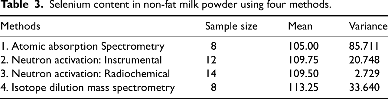
Four different analytical methods were used to estimate the selenium in non-fat milk powder and the mean and variance are reported in Table 3. The data are taken from Eberhardt et al. ⁴ Application of Bartlett’s test by Jordan and Krishnamoorthy ²³ has shown that the variances are significantly different, and so the $t$ -test for the mean based on the pooled data is not appropriate.

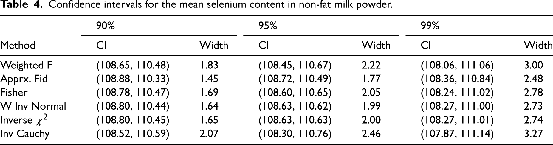
The 90, 95 and 99% CIs based on different methods are reported in Table 4. All CIs are in agreement. The inverse ${\chi }^2$ , Fisher and the weighted inverse normal methods produced practically the same confidence interval. As indicated by the simulation studies in the preceding section, the inverse Cauchy intervals are wider than all other CIs for this example. Finding the 95% CI using the Fisher method is described graphically in Figure 1. The R function CI.normal.Cmean(n, xb, sq, cl,method) provided in the supplementary file was used to compute CIs by the Fisher, weighted inverse normal, inverse Cauchy and inverse ${\chi }^2$ methods.

Table 4.

Confidence intervals for the mean selenium content in non-fat milk powder.

	90%		95%		99%
Method	CI	Width	CI	Width	CI	Width
Weighted F	(108.65, 110.48)	1.83	(108.45, 110.67)	2.22	(108.06, 111.06)	3.00
Apprx. Fid	(108.88, 110.33)	1.45	(108.72, 110.49)	1.77	(108.36, 110.84)	2.48
Fisher	(108.78, 110.47)	1.69	(108.60, 110.65)	2.05	(108.24, 111.02)	2.78
W Inv Normal	(108.80, 110.44)	1.64	(108.63, 110.62)	1.99	(108.27, 111.00)	2.73
Inverse ${\chi }^2$	(108.80, 110.45)	1.65	(108.63, 110.63)	2.00	(108.27, 111.01)	2.74
Inv Cauchy	(108.52, 110.59)	2.07	(108.30, 110.76)	2.46	(107.87, 111.14)	3.27

4. Common coefficient of variation

The CV is defined as the ratio of the standard deviation to the mean, $\sigma /\mu$ , and is defined only for distributions of positive random variables. For a normal population, the ratio of the mean to the standard deviation has to be on the order of three or more, for the probability of a negative value is negligible. This means that $\mu -3\sigma >0$ , or the CV $\sigma /\mu$ must be at most $1/3$ in practical situations where the CV is a suitable measure of variability. ²⁹

4.1. A Test for a CV

Consider a sample $X_1,\dots ,X_n$ from a $N(\mu ,{\sigma }^2)$ population. The population CV is defined as $\tau =\sigma /\mu .$ Let $(\overline{X},S^2)$ be the (mean, variance) based on the sample and let $(\overline{x},s^2)$ be an observed value of $(\overline{X},S^2)$ . The sample CV is given by $\hat{\tau }=S/\overline{X}$ . To derive a test for $H_0:\tau ={\tau }_0\mathrm{vs}.H_a:\tau >{\tau }_0,$ based on the sample, we first note that $\sqrt{n}\overline{X}/S\sim t_m(\sqrt{n}/\tau ),$ where $t_m(\delta )$ denotes the noncentral $t$ random variable with df $m=n-1$ and the noncentrality parameter $\delta$ . Let $\zeta =1/\tau$ and $\hat{\zeta }=\overline{X}/S$ . Hypothesis test or CI for $\tau$ can be readily obtained from the one for $\zeta$ . In particular, for testing $H_0:\zeta ={\zeta }_0$ vs. $H_{:}\zeta >{\zeta }_0$ , the $p$ -value is given by

$$P=P(t_m(\sqrt{n}{\zeta }_0)\ge \sqrt{n}{\hat{\zeta }}_0)$$

(5) where ${\hat{\zeta }}_0=\overline{x}/s$ is an observed value of $\hat{\zeta }$ . A CI for $\zeta$ can be obtained by inverting one-sided tests.

4.1.1. Confidence intervals for $\tau$ based on a combined test

Let $({\overline{X}}_i,S_i^2)$ denote the (mean, variance) based on the $i$ th sample, and $({\overline{x}}_i,s_i^2)$ be an observed value of $({\overline{X}}_i,S_i^2)$ , $i=1,\dots ,k$ . Consider testing $H_0:\zeta ={\zeta }_0\mathrm{vs}.H_a:\zeta >{\zeta }_0$ using the $i$ th sample. For an observed value ${\hat{\zeta }}_{i0}={\overline{x}}_i/s_i$ , the null hypothesis will be rejected whenever the $p$ -value

$$P_i=P(t_{m_i}(\sqrt{n_i}{\zeta }_0)\ge \sqrt{n_i}{\hat{\zeta }}_{i0})<\alpha$$

(6) and it is an exact level $\alpha$ test. A combined test for $H_0:\zeta ={\zeta }_0\mathrm{vs}.H_a:\zeta >{\zeta }_0,$ can be obtained using a combinations of the $p$ -values $P_1,\dots ,P_k$ in Table 1, and it can be inverted to find a lower confidence limit for $\zeta =1/\tau$ . Similarly, by inverting a left-tailed test for $\zeta$ , a lower confidence limit for $\tau$ can be obtained. Reciprocal of these one-sided confidence limits form a CI for $\tau$ .

4.2. Coefficient of variation: Coverage and precision studies

Forkman ¹⁰ proposed an approximate CI for a common CV and Tian ⁹ also proposed a generalized fiducial CI for a common CV. We did not include these CIs for comparison study as our preliminary studies indicated that these CIs are less accurate than those based on the combined tests (see Murshed ³⁰ for details).

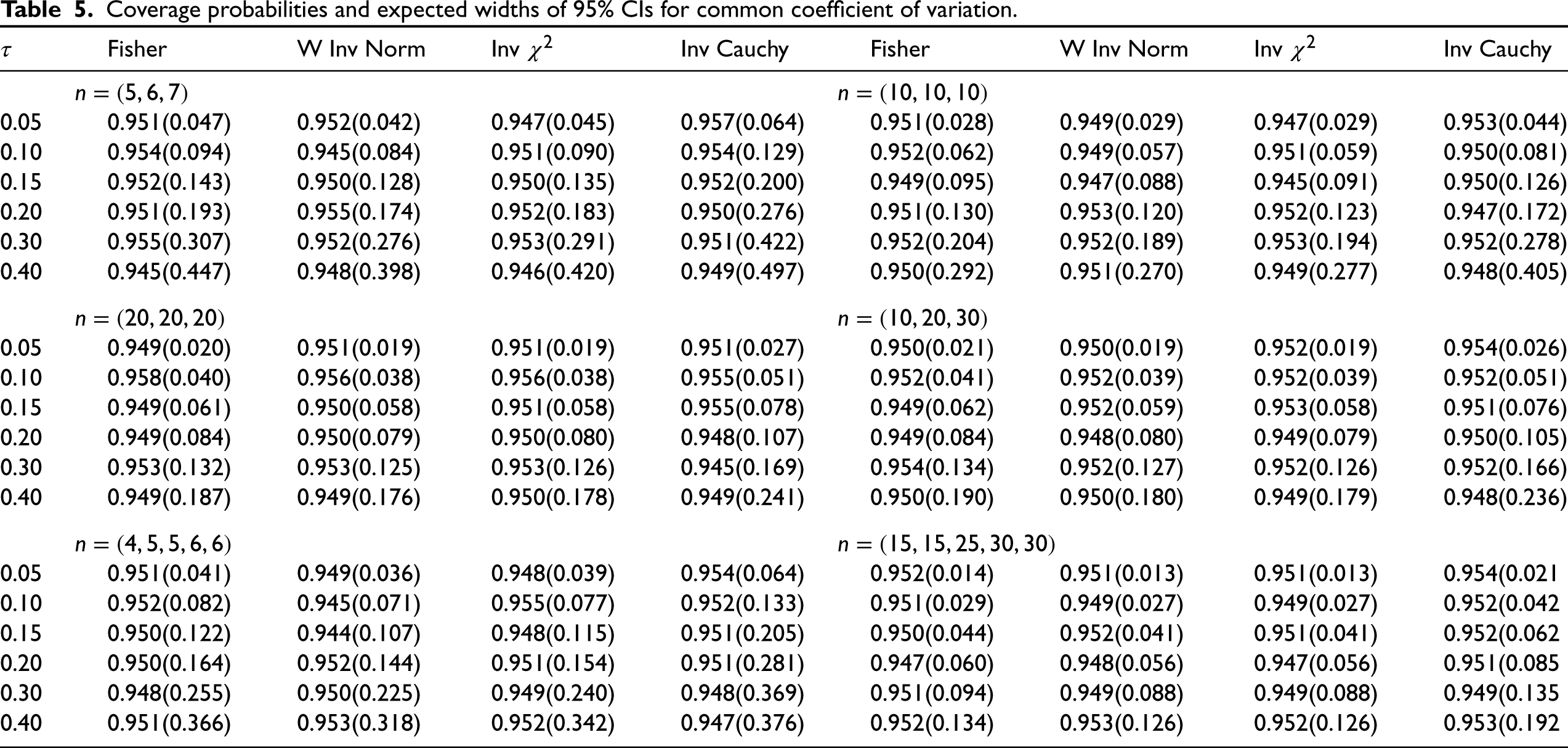
To compare all other CIs, we chose samples of sizes from small to moderate, number of sources $k=3$ and 5, and $\tau =0.05,0.10,0.15,0.20,0.30$ and 0.40. From the reported coverage probabilities and expected widths in Table 5, we observe the following. Among the CIs based on combined tests, inverse Cauchy method produced CIs that are much wider than the other three CIs for almost all cases. There are only little differences among the precisions of the CIs based on the inverse ${\chi }^2$ test and the weighted inverse normal test. There are a few cases where the CIs based on the weighted inverse normal test are narrower than the corresponding CIs based on the inverse ${\chi }^2$ test. In general, Fisher’s CIs are little wider than the CIs based on the weighted inverse normal test and those based on the inverse ${\chi }^2$ test. Thus, the CIs based on the weighted inverse normal test are preferable to others.

Remark 2. Liu and Xu ¹³ developed CIs for the common CV using the approach called confidence distributions which is “Neymannian interpretation” of Fisher’s fiducial distribution, and so closely related to the fiducial approach. The proposed CIs in their paper are also exact in the frequentist sense, except that Monte Carlo simulation is required to find CIs. The CIs based on confidence distributions and the ones based on our numerical approach with the Fisher combined test are the same. This is also supported by the agreement of coverage probabilities and expected widths reported in our Table 5 and those in Table 1 of Liu and Xu ¹³ for the cases of sample sizes $(10,10,10),$ $(20,20,20)$ and $(10,20,30)$ .

Table 5.

Coverage probabilities and expected widths of 95% CIs for common coefficient of variation.

$\tau$	Fisher	W Inv Norm	Inv ${\chi }^2$	Inv Cauchy	Fisher	W Inv Norm	Inv ${\chi }^2$	Inv Cauchy
	$n=(5,6,7)$				$n=(10,10,10)$
0.05	0.951(0.047)	0.952(0.042)	0.947(0.045)	0.957(0.064)	0.951(0.028)	0.949(0.029)	0.947(0.029)	0.953(0.044)
0.10	0.954(0.094)	0.945(0.084)	0.951(0.090)	0.954(0.129)	0.952(0.062)	0.949(0.057)	0.951(0.059)	0.950(0.081)
0.15	0.952(0.143)	0.950(0.128)	0.950(0.135)	0.952(0.200)	0.949(0.095)	0.947(0.088)	0.945(0.091)	0.950(0.126)
0.20	0.951(0.193)	0.955(0.174)	0.952(0.183)	0.950(0.276)	0.951(0.130)	0.953(0.120)	0.952(0.123)	0.947(0.172)
0.30	0.955(0.307)	0.952(0.276)	0.953(0.291)	0.951(0.422)	0.952(0.204)	0.952(0.189)	0.953(0.194)	0.952(0.278)
0.40	0.945(0.447)	0.948(0.398)	0.946(0.420)	0.949(0.497)	0.950(0.292)	0.951(0.270)	0.949(0.277)	0.948(0.405)
	$n=(20,20,20)$				$n=(10,20,30)$
0.05	0.949(0.020)	0.951(0.019)	0.951(0.019)	0.951(0.027)	0.950(0.021)	0.950(0.019)	0.952(0.019)	0.954(0.026)
0.10	0.958(0.040)	0.956(0.038)	0.956(0.038)	0.955(0.051)	0.952(0.041)	0.952(0.039)	0.952(0.039)	0.952(0.051)
0.15	0.949(0.061)	0.950(0.058)	0.951(0.058)	0.955(0.078)	0.949(0.062)	0.952(0.059)	0.953(0.058)	0.951(0.076)
0.20	0.949(0.084)	0.950(0.079)	0.950(0.080)	0.948(0.107)	0.949(0.084)	0.948(0.080)	0.949(0.079)	0.950(0.105)
0.30	0.953(0.132)	0.953(0.125)	0.953(0.126)	0.945(0.169)	0.954(0.134)	0.952(0.127)	0.952(0.126)	0.952(0.166)
0.40	0.949(0.187)	0.949(0.176)	0.950(0.178)	0.949(0.241)	0.950(0.190)	0.950(0.180)	0.949(0.179)	0.948(0.236)
	$n=(4,5,5,6,6)$				$n=(15,15,25,30,30)$
0.05	0.951(0.041)	0.949(0.036)	0.948(0.039)	0.954(0.064)	0.952(0.014)	0.951(0.013)	0.951(0.013)	0.954(0.021
0.10	0.952(0.082)	0.945(0.071)	0.955(0.077)	0.952(0.133)	0.951(0.029)	0.949(0.027)	0.949(0.027)	0.952(0.042
0.15	0.950(0.122)	0.944(0.107)	0.948(0.115)	0.951(0.205)	0.950(0.044)	0.952(0.041)	0.951(0.041)	0.952(0.062
0.20	0.950(0.164)	0.952(0.144)	0.951(0.154)	0.951(0.281)	0.947(0.060)	0.948(0.056)	0.947(0.056)	0.951(0.085
0.30	0.948(0.255)	0.950(0.225)	0.949(0.240)	0.948(0.369)	0.951(0.094)	0.949(0.088)	0.949(0.088)	0.949(0.135
0.40	0.951(0.366)	0.953(0.318)	0.952(0.342)	0.947(0.376)	0.952(0.134)	0.953(0.126)	0.952(0.126)	0.953(0.192

4.3. Example for coefficient of variation

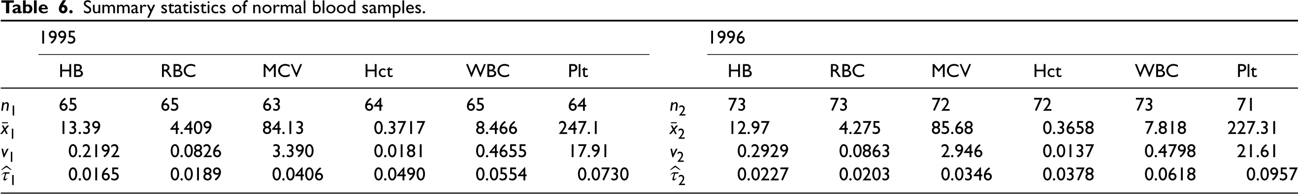
For the purpose of promoting the quality and setting standards of medical laboratory technology, Hong Kong Medical Technology Association conducted a quality assurance program for medical laboratories in Hong Kong in 1989. In the specialty of hematology and serology, one normal and one abnormal hematology and serology blood samples were sent to participants for measurements of Hb, RBC, MCV, Hct, WBC, and Platelet in each survey. The summary statistics of data on normal blood samples collected from the third surveys of 1995 and 1996 are given in Fung and Tsang, ³¹ and they are reproduced here in Table 6. Here, $v_i^2=(n_i-1)s_i^2/n_i$ is the maximum likelihood estimator (MLE) of ${\sigma }_i^2$ . The data were also analyzed by Tian ⁹ and Krishnamoorthy and Lee. ³²

Table 6.

Summary statistics of normal blood samples.

	1995							1996
	HB	RBC	MCV	Hct	WBC	Plt		HB	RBC	MCV	Hct	WBC	Plt
$n_1$	65	65	63	64	65	64	$n_2$	73	73	72	72	73	71
${\overline{x}}_1$	13.39	4.409	84.13	0.3717	8.466	247.1	${\overline{x}}_2$	12.97	4.275	85.68	0.3658	7.818	227.31
$v_1$	0.2192	0.0826	3.390	0.0181	0.4655	17.91	$v_2$	0.2929	0.0863	2.946	0.0137	0.4798	21.61
${\hat{\tau }}_1$	0.0165	0.0189	0.0406	0.0490	0.0554	0.0730	${\hat{\tau }}_2$	0.0227	0.0203	0.0346	0.0378	0.0618	0.0957

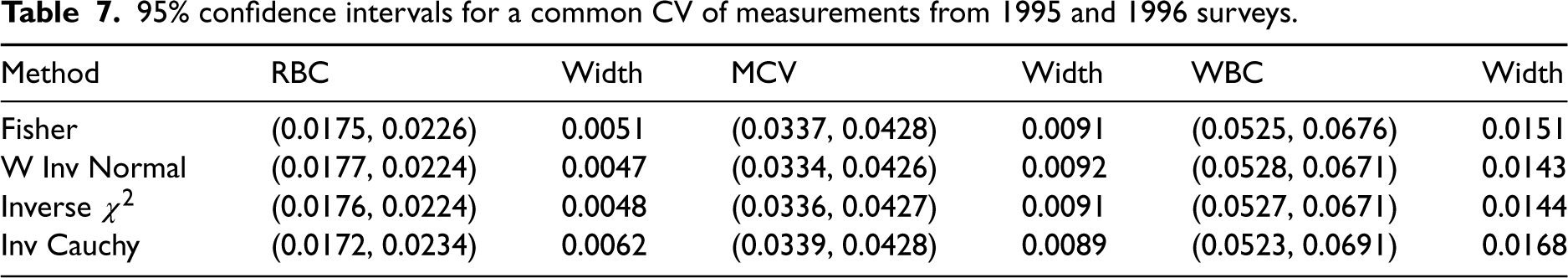
The tests and CIs by Krishnamoorthy and Lee ³² indicated that coefficients of variation of measurements in 1995 and 1996 are the same for variables RBC, MCV and WBC. For these three variables, we estimated CIs for the common CV using different approaches and reported them in Table 7. Since the numbers of measurements are quite large, all methods, except inverse Cauchy, produced similar CIs for common coefficients of variation of different pairs. A cursory glance of Table 7 shows that the inverse Cauchy CIs are somewhat different from others. R functions that were used to compute CIs for a common $\tau$ are provided in a supplementary file. The R function CI.common.CV(n, zetah, cl, method) provided in the supplementary file was used to compute CIs by the Fisher, weighted inverse normal, inverse Cauchy and inverse ${\chi }^2$ methods.

Table 7.

95% confidence intervals for a common CV of measurements from 1995 and 1996 surveys.

Method	RBC	Width	MCV	Width	WBC	Width
Fisher	(0.0175, 0.0226)	0.0051	(0.0337, 0.0428)	0.0091	(0.0525, 0.0676)	0.0151
W Inv Normal	(0.0177, 0.0224)	0.0047	(0.0334, 0.0426)	0.0092	(0.0528, 0.0671)	0.0143
Inverse ${\chi }^2$	(0.0176, 0.0224)	0.0048	(0.0336, 0.0427)	0.0091	(0.0527, 0.0671)	0.0144
Inv Cauchy	(0.0172, 0.0234)	0.0062	(0.0339, 0.0428)	0.0089	(0.0523, 0.0691)	0.0168

5. Common mean of several lognormal populations

Consider $k$ log-normal populations with parameters $({\mu }_1,{\sigma }_1),\dots ,({\mu }_k,{\sigma }_k)$ . Assume that the means of these $k$ populations are the same $\exp (\eta )$ , where $\eta =({\mu }_i+.5{\sigma }_i^2)$ , $i=1,\dots ,k$ . Tian and Wu ⁶ proposed a GV approach to find a CI for the common mean of several log-normal distributions. We shall now describe an efficient test for the lognormal mean and combined tests based on this one-sample test. The combined tests can be inverted to find CIs for a common mean of several lognormal populations.

Let $X_{i1},\dots ,X_{i{n}_i}$ be a log-transformed sample from a lognormal distribution with parameters ${\mu }_i$ and ${\sigma }_i$ , $i=1,\dots ,k$ . Recall that $X_{i1},\dots ,X_{i{n}_i}\sim N({\mu }_i,{\sigma }_i^2)$ , $i=1,\dots ,k$ . Since the common mean of lognormal distributions is given by $\exp (\eta )$ with $\eta ={\mu }_i+\frac{1}{2}{\sigma }_i^2$ , $i=1,\dots ,k$ , it is enough to find a CI for $\eta$ . Let $({\overline{X}}_i,S_i^2)$ denote the (mean, variance) based on a sample of size $n_i$ from the $i$ th population.

5.1. The modified likelihood ratio test for a lognormal mean

To describe the modified likelihood ratio test (MLRT) by Wu et al. ³³ for a single sample, let $(w_1,w_2)=(\sum _{i=1}^n{X}_i,\sum _{i=1}^n{X}_i^2)$ . The MLEs are ${\hat{\sigma }}^2={\overline{w}}_2-{\overline{w}}_1^2\mathrm{and}\hat{\eta }={\overline{w}}_1+\frac{1}{2}{\hat{\sigma }}^2,$ where ${\overline{w}}_1=w_1/n$ and ${\overline{w}}_2=w_2/n$ . For fixed $\eta$ , the constrained maximum likelihood estimate of ${\sigma }^2$ is ${\hat{\sigma }}_{\eta }^2=2\{(\eta +1{)}^2+{\overline{w}}_2-2\eta {\overline{w}}_1-2\eta {\}}^{1/2}-2.$ Define

$$r(\eta )=\mathrm{sgn}(\hat{\eta }-\eta ){\{n\ln \frac{{\hat{\sigma }}_{\eta }^2}{{\hat{\sigma }}^2}+n({\overline{w}}_1-\eta +{\hat{\sigma }}_{\eta }^2/2)\}}^{\frac{1}{2}}$$

(7) and

$$u(\eta )=\sqrt{n}(\hat{\eta }-\eta )\left(\frac{\hat{\sigma }}{{\hat{\sigma }}_{\eta }^3}\right)/\sqrt{\frac{1}{2}+\frac{1}{{\hat{\sigma }}_{\eta }^2}}$$

(8) For testing $H_0:\eta ={\eta }_0$ vs. $H_a:\eta >{\eta }_0$ , the MLRT statistic is given by

$$r^{*}({\eta }_0)=r({\eta }_0)+\frac{1}{r({\eta }_0)}\ln \frac{u({\eta }_0)}{r({\eta }_0)}$$

(9) which follows a standard normal distribution asymptotically. This asymptotic result has third-order accuracy, and is valid even for small samples. The $p$ -value of the MLRT is given by

$$P(Z>r^{*}({\eta }_0))=1-\mathrm{\Phi }(r^{*}({\eta }_0))$$

(10) where $\mathrm{\Phi }$ is the standard normal distribution function.

5.2. Combined tests for a common lognormal mean

To develop a combined test for a common mean of several lognormal distributions, let us suppose that the means of all the $k$ populations are the same. That is, $\exp ({\mu }_1+\frac{1}{2}{\sigma }_1^2)=\dots =\exp ({\mu }_k+\frac{1}{2}{\sigma }_k^2)$ , or equivalently, $\eta ={\mu }_1+\frac{1}{2}{\sigma }_1^2=\dots ={\mu }_k+\frac{1}{2}{\sigma }_k^2.$ Let $P_i({\eta }_0)$ denote the $p$ -value for testing

$$H_0:\eta ={\eta }_0\mathrm{vs}.H_a:\eta >{\eta }_0$$

based on the $i$ th sample. These $p$ -values can be combined using any of the methods described in Section 2 to arrive at a single test for the common mean of several lognormal populations. The combined tests may be inverted using Algorithm 1 to find a CI for a common mean of lognormal distributions.

5.3. Lognormal: Simulation studies

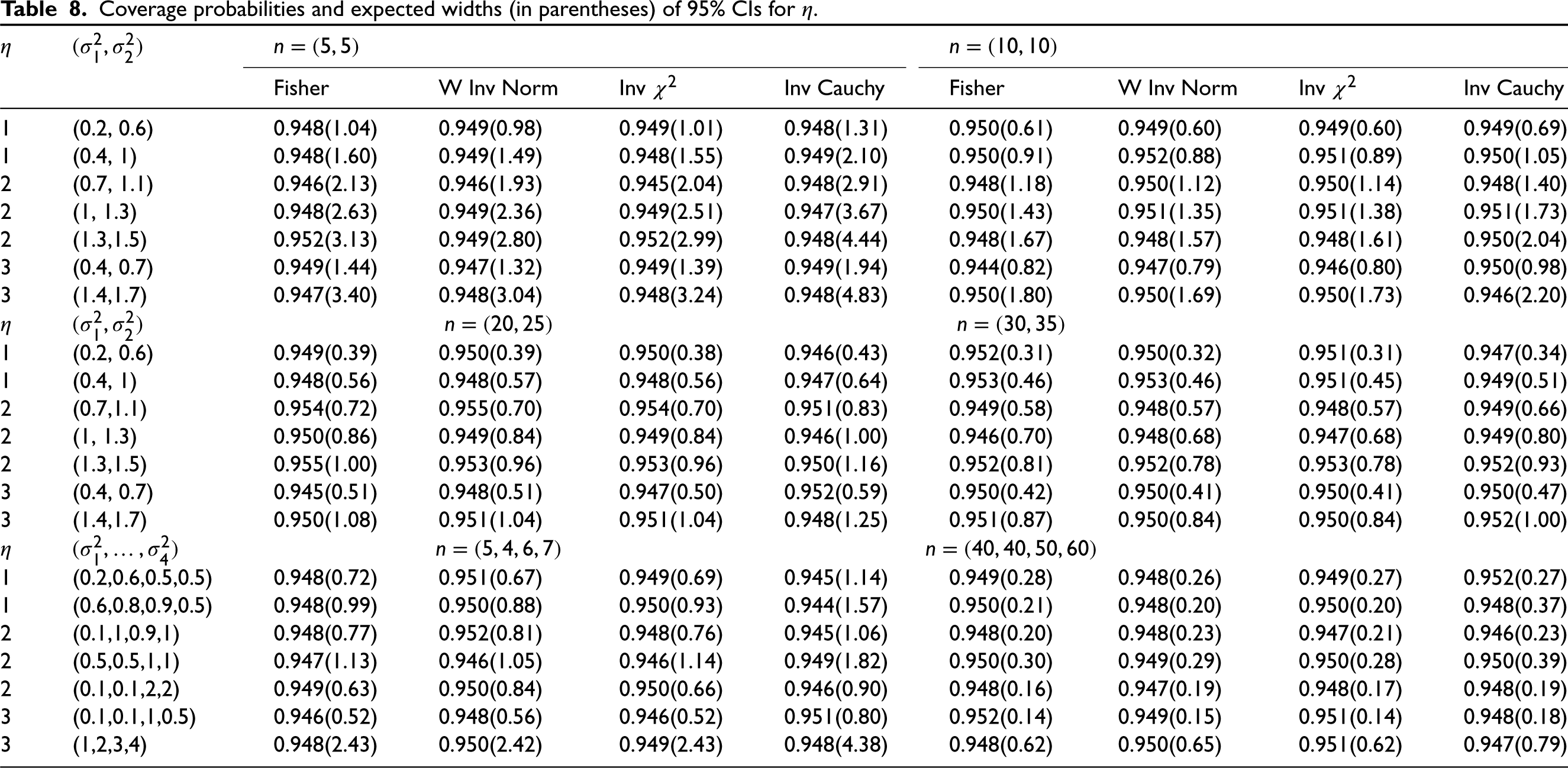
There are other approximate CIs based on the MOVER approach and fiducial approach. ⁶ Our preliminary investigations indicated that these CIs are not so accurate as those based on combined tests, and so we do not include these CIs in our comparison study. Murshed ³⁰ has included these CIs for comparison study. We estimated the coverage probabilities and expected widths of all CIs based on combined tests for a common mean of several lognormal distributions and presented them in Table 8. We chose $\eta ={\mu }_i+.5{\sigma }_i^2$ as 1, 2, and 3, and different combinations for values of $({\sigma }_1^2,\dots ,{\sigma }_k^2)$ . We considered only cases of $k=2$ and 4. All simulation estimates are based on 10,000 runs. Since the MLRT for testing a lognormal mean based on a single sample is very accurate even for small samples, the coverage probabilities of CIs based on combined tests are close to the nominal level for all cases. The inverse Cauchy CIs are wider than all CIs for almost all cases. The CIs based on the inverse ${\chi }^2$ test and the weighted inverse normal test are very similar in terms of coverage probability. The CIs based on the Fisher test and the inverse ${\chi }^2$ test are quite comparable, and both are equally efficient. The CIs based on the weighted inverse normal test are somewhat less efficient than the other two CIs based on the Fisher test and the inverse ${\chi }^2$ test for some cases; for example, see the results for $n=(40,40,50,60)$ in Table 8. On an overall basis, the CIs based on the weighted inverse normal test and the inverse ${\chi }^2$ are recommended for applications.

Table 8.

Coverage probabilities and expected widths (in parentheses) of 95% CIs for $\eta$ .

$\eta$	$({\sigma }_1^2,{\sigma }_2^2)$	$n=(5,5)$				$n=(10,10)$
		Fisher	W Inv Norm	Inv ${\chi }^2$	Inv Cauchy	Fisher	W Inv Norm	Inv ${\chi }^2$	Inv Cauchy
1	(0.2, 0.6)	0.948(1.04)	0.949(0.98)	0.949(1.01)	0.948(1.31)	0.950(0.61)	0.949(0.60)	0.949(0.60)	0.949(0.69)
1	(0.4, 1)	0.948(1.60)	0.949(1.49)	0.948(1.55)	0.949(2.10)	0.950(0.91)	0.952(0.88)	0.951(0.89)	0.950(1.05)
2	(0.7, 1.1)	0.946(2.13)	0.946(1.93)	0.945(2.04)	0.948(2.91)	0.948(1.18)	0.950(1.12)	0.950(1.14)	0.948(1.40)
2	(1, 1.3)	0.948(2.63)	0.949(2.36)	0.949(2.51)	0.947(3.67)	0.950(1.43)	0.951(1.35)	0.951(1.38)	0.951(1.73)
2	(1.3,1.5)	0.952(3.13)	0.949(2.80)	0.952(2.99)	0.948(4.44)	0.948(1.67)	0.948(1.57)	0.948(1.61)	0.950(2.04)
3	(0.4, 0.7)	0.949(1.44)	0.947(1.32)	0.949(1.39)	0.949(1.94)	0.944(0.82)	0.947(0.79)	0.946(0.80)	0.950(0.98)
3	(1.4,1.7)	0.947(3.40)	0.948(3.04)	0.948(3.24)	0.948(4.83)	0.950(1.80)	0.950(1.69)	0.950(1.73)	0.946(2.20)
$\eta$	$({\sigma }_1^2,{\sigma }_2^2)$	$n=(20,25)$			$n=(30,35)$
1	(0.2, 0.6)	0.949(0.39)	0.950(0.39)	0.950(0.38)	0.946(0.43)	0.952(0.31)	0.950(0.32)	0.951(0.31)	0.947(0.34)
1	(0.4, 1)	0.948(0.56)	0.948(0.57)	0.948(0.56)	0.947(0.64)	0.953(0.46)	0.953(0.46)	0.951(0.45)	0.949(0.51)
2	(0.7,1.1)	0.954(0.72)	0.955(0.70)	0.954(0.70)	0.951(0.83)	0.949(0.58)	0.948(0.57)	0.948(0.57)	0.949(0.66)
2	(1, 1.3)	0.950(0.86)	0.949(0.84)	0.949(0.84)	0.946(1.00)	0.946(0.70)	0.948(0.68)	0.947(0.68)	0.949(0.80)
2	(1.3,1.5)	0.955(1.00)	0.953(0.96)	0.953(0.96)	0.950(1.16)	0.952(0.81)	0.952(0.78)	0.953(0.78)	0.952(0.93)
3	(0.4, 0.7)	0.945(0.51)	0.948(0.51)	0.947(0.50)	0.952(0.59)	0.950(0.42)	0.950(0.41)	0.950(0.41)	0.950(0.47)
3	(1.4,1.7)	0.950(1.08)	0.951(1.04)	0.951(1.04)	0.948(1.25)	0.951(0.87)	0.950(0.84)	0.950(0.84)	0.952(1.00)
$\eta$	$({\sigma }_1^2,\dots ,{\sigma }_4^2)$	$n=(5,4,6,7)$			$n=(40,40,50,60)$
1	(0.2,0.6,0.5,0.5)	0.948(0.72)	0.951(0.67)	0.949(0.69)	0.945(1.14)	0.949(0.28)	0.948(0.26)	0.949(0.27)	0.952(0.27)
1	(0.6,0.8,0.9,0.5)	0.948(0.99)	0.950(0.88)	0.950(0.93)	0.944(1.57)	0.950(0.21)	0.948(0.20)	0.950(0.20)	0.948(0.37)
2	(0.1,1,0.9,1)	0.948(0.77)	0.952(0.81)	0.948(0.76)	0.945(1.06)	0.948(0.20)	0.948(0.23)	0.947(0.21)	0.946(0.23)
2	(0.5,0.5,1,1)	0.947(1.13)	0.946(1.05)	0.946(1.14)	0.949(1.82)	0.950(0.30)	0.949(0.29)	0.950(0.28)	0.950(0.39)
2	(0.1,0.1,2,2)	0.949(0.63)	0.950(0.84)	0.950(0.66)	0.946(0.90)	0.948(0.16)	0.947(0.19)	0.948(0.17)	0.948(0.19)
3	(0.1,0.1,1,0.5)	0.946(0.52)	0.948(0.56)	0.946(0.52)	0.951(0.80)	0.952(0.14)	0.949(0.15)	0.951(0.14)	0.948(0.18)
3	(1,2,3,4)	0.948(2.43)	0.950(2.42)	0.949(2.43)	0.948(4.38)	0.948(0.62)	0.950(0.65)	0.951(0.62)	0.947(0.79)

5.4. Lognormal: An example

We shall now illustrate the methods using the example given in Tian and Wu ⁶ and also discussed in Krishnamoorthy and Oral. ⁷ The pharmacokinetics data were obtained from alcohol interaction study in men. For illustrative purpose, we use the measurements on maximum concentration ( $Cmax$ ) and compare the active treatment groups considered in Tian and Wu. ⁶ The statistics based on the log-transformed data are as follows:

$$n_1=n_2=n_3=22,({\overline{x}}_1,{\overline{x}}_2,{\overline{x}}_3)=(2.601,2.596,2.599)\mathrm{and}(s_1^2,s_2^2,s_3^2)=(0.24,0.20,0.17)$$

The MLRT by Krishnamoorthy and Oral ⁷ indicated that $H_0:{\eta }_1={\eta }_2={\eta }_3$ is tenable. Since the group means are not significantly different, it maybe desired to the find the common mean of these three groups.

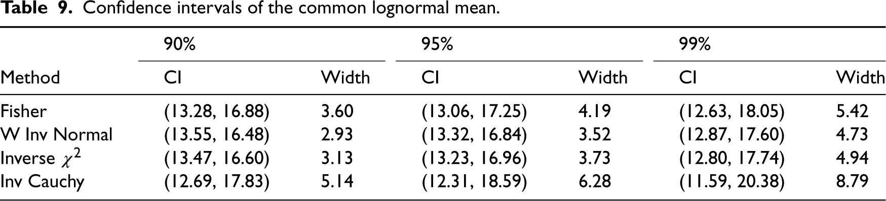
We estimated 90, 95 and 99% CIs for the common mean of these three groups and reported them in the following Table 9.

Table 9.

Confidence intervals of the common lognormal mean.

	90%		95%		99%
Method	CI	Width	CI	Width	CI	Width
Fisher	(13.28, 16.88)	3.60	(13.06, 17.25)	4.19	(12.63, 18.05)	5.42
W Inv Normal	(13.55, 16.48)	2.93	(13.32, 16.84)	3.52	(12.87, 17.60)	4.73
Inverse ${\chi }^2$	(13.47, 16.60)	3.13	(13.23, 16.96)	3.73	(12.80, 17.74)	4.94
Inv Cauchy	(12.69, 17.83)	5.14	(12.31, 18.59)	6.28	(11.59, 20.38)	8.79

Note that the inverse normal method produced the shortest CIs while the inverse Cauchy method produced the widest CIs for all three nominal confidence levels. We used the R function CI.lnorm.cmean = function(n, xb, sq, cl, method) provided in the supplementary file to compute CIs by the Fisher, inverse chi-square and the weighted inverse normal methods.

6. Common correlation coefficient

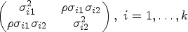
The problem of estimating a common correlation coefficient of several bivariate normal populations has been addressed by Donner and Rosner, ¹¹ Paul ³⁴ and Tian and Wilding. ¹² These authors have proposed some approximate tests and confidence intervals for a common correlation coefficient. To describe the problem formally, let ${\mathit{X}}_{i1},\dots ,{\mathit{X}}_{i{n}_i}$ be a sample from a bivariate normal distribution with mean vector ${\mathit{\mu }}_i$ and variance-covariance matrix

$$\left(\begin{array}{cc}{\sigma }_{i1}^2& \rho {\sigma }_{i1}{\sigma }_{i2}\\ \rho {\sigma }_{i1}{\sigma }_{i2}& {\sigma }_{i2}^2\end{array}\right),i=1,\dots ,k$$

Let ${\mathit{S}}_i=(s_{i,lj})$ be the sample variance-covariance matrix based on the $i$ th sample. Then the sample correlation coefficient is given by $R_i=s_{i,12}/\sqrt{s_{i,11}{s}_{i,22}}$ , $i=1,\dots ,k.$ In the following, we first describe the CI given in Donner and Rosner ¹¹ that was obtained by combining the Fisher $Z$ statistics based on individual samples.

6.1. A CI for $\rho$ based on Fisher’s $Z$ statistics

Using the Fisher $z$ -transformation of $R_i$ ’s, we have the asymptotic result that

$$Z_i={\tanh }^{-1}(R_i)=\frac{1}{2}\ln \frac{1+R_i}{1-R_i}\sim N({\mu }_{\rho },(n_i-3{)}^{-1})$$

(11) where ${\mu }_{\rho }={\tanh }^{-1}(\rho )=\frac{1}{2}\ln \frac{1+\rho }{1-\rho }$ . Using this distributional result along with the fact that $Z_i$ ’s are independent, under $H_0:\rho ={\rho }_0$ , $Z_c=\sum _{i=1}^k{Q}_i{Z}_i\sim N({\mu }_{{\rho }_0},1/(N-3k)),$ where $Q_i=\frac{(n_i-3)}{\sum _{j=1}^k(n_j-3)}$ and $N=\sum _{i=1}^k{n}_i.$ Thus, this combined test rejects $H_0$ in favor of $H_a:\rho >{\rho }_0$ if $\sqrt{N-3k}(Z_c-{\mu }_{{\rho }_0})>z_{1-\alpha }$ , or equivalently the $p$ -value $1-\mathrm{\Phi }(\sqrt{N-3k}(Z_c-{\mu }_{{\rho }_0}))<\alpha$ .

A $(1-2\alpha )$ CI for ${\mu }_{\rho }$ , follows from the distribution of $Z_c$ , and is given by

$$(L_{{\mu }_{\rho }},U_{{\mu }_{\rho }})=\sum _{i=1}^k{Q}_i{Z}_i\pm z_{1-\alpha }\sqrt{\frac{1}{N-3k}}$$

(12) where $N=\sum _{i=1}^k{n}_i$ . As ${\mu }_{\rho }$ is an increasing function of $\rho$ , a CI for $\rho$ can be deduced from the above one for $\rho$ as $(\tanh (L_{{\mu }_{\rho }}),\tanh (U_{{\mu }_{\rho }})).$ Donner and Rosner ¹¹ have proposed this CI and we refer to this CI as the $z$ -interval for $\rho$ .

6.2. CIs based combined tests

Let $z_i$ be an observed value of $Z_i$ . That is, $z_i=\frac{1}{2}\ln (\frac{1+r_i}{1-r_i})$ , where $r_i$ is an observed value of $R_i$ , $i=1,\dots ,k$ . Furthermore, the $p$ -value for testing $H_0:\rho ={\rho }_0\mathrm{vs}.H_a:\rho >{\rho }_0$ on the basis of the $i$ th sample is given by

$$P_i=P(Z_i>z_i|n_i,{\rho }_0)=1-\mathrm{\Phi }(\sqrt{n_i-3}(z_i-{\mu }_{{\rho }_0}))$$

(13) where $\mathrm{\Phi }$ is the standard normal distribution function. The above $p$ -values can be combined using one of the methods in Section 2 to arrive at a single test, and the test can be inverted to get a CI for the common $\rho$ . Remark 3. It should be noted that there are other tests for $\rho$ that are more accurate than the Fisher test are available in the literature; see Krishnamoorthy and Xia. ³⁵ However, the above Fisher’s test is simple and commonly used in applications, and so we proceed with the above test.

6.3. Common correlation: Coverage and precision studies

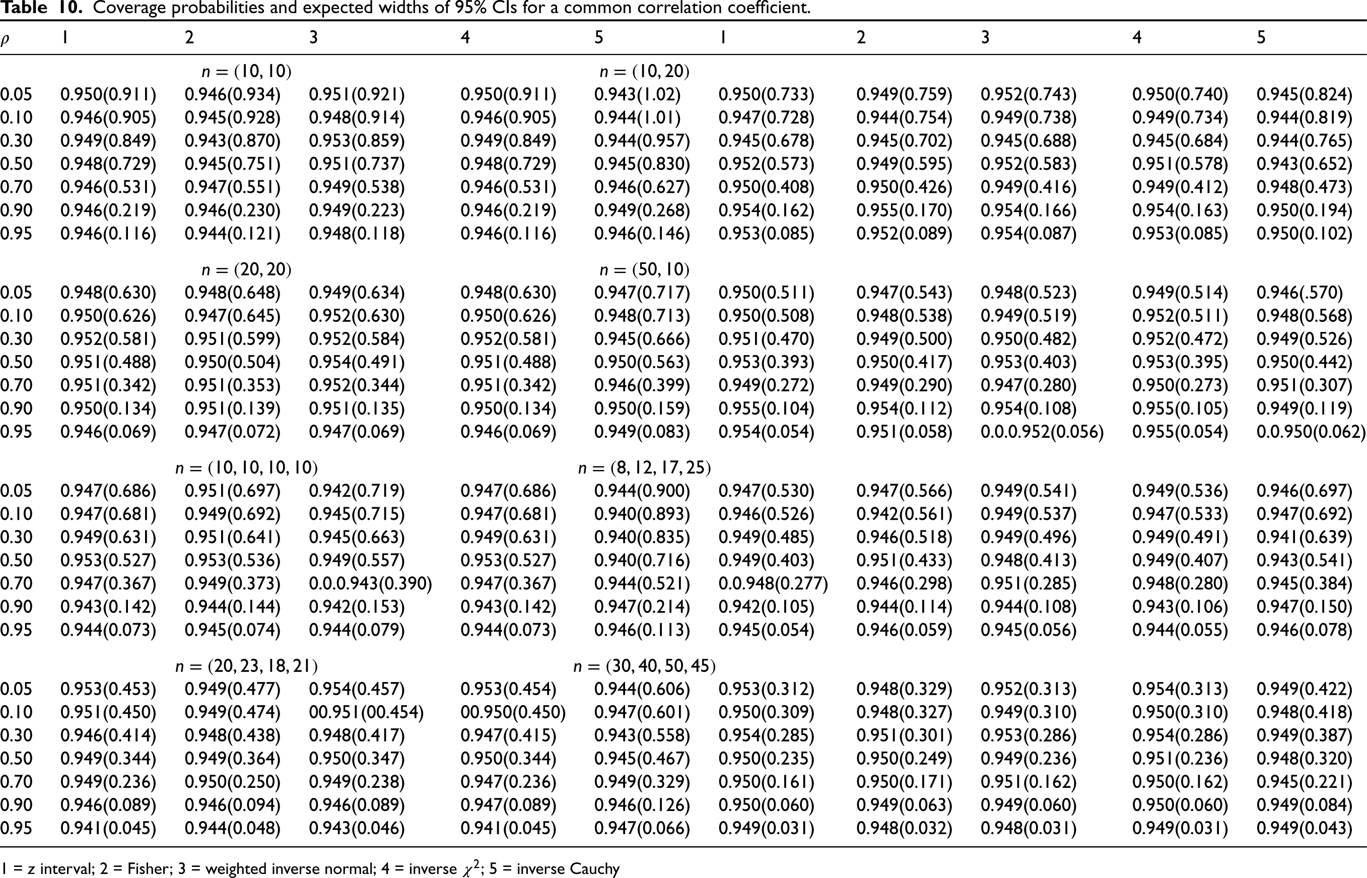
The CIs for a common correlation coefficient are based on combined tests where individual tests are approximate. Even though the individual Fisher tests are known to be accurate even for small samples, we need to compare the CIs based on the combined tests and Donner and Rosner’s ¹¹ approach in terms of precision. We estimated the coverage probabilities and expected widths of all CIs using Monte Carlo simulation with 10,000 runs and reported them in Table 10. The estimated coverage probabilities in Table 10 indicate that the CIs based on all combined tests are practically exact. The inverse Cauchy CIs are much wider than all other CIs for all cases. The estimated coverage probabilities and expected widths indicate that the Donner and Rosner CIs and the ones based on the weighted inverse normal test are practically the same in terms of coverage probability and precision. The CI based on the inverse ${\chi }^2$ test and the one based on the weighted inverse normal test are similar in most cases, and the latter is better than the former in a few cases. Overall, Donner and Rosner’s CI is preferable to others for simplicity, accuracy and efficiency.

Table 10.

Coverage probabilities and expected widths of 95% CIs for a common correlation coefficient.

$\rho$	1	2	3	4	5	1	2	3	4	5
	$n=(10,10)$			$n=(10,20)$
0.05	0.950(0.911)	0.946(0.934)	0.951(0.921)	0.950(0.911)	0.943(1.02)	0.950(0.733)	0.949(0.759)	0.952(0.743)	0.950(0.740)	0.945(0.824)
0.10	0.946(0.905)	0.945(0.928)	0.948(0.914)	0.946(0.905)	0.944(1.01)	0.947(0.728)	0.944(0.754)	0.949(0.738)	0.949(0.734)	0.944(0.819)
0.30	0.949(0.849)	0.943(0.870)	0.953(0.859)	0.949(0.849)	0.944(0.957)	0.945(0.678)	0.945(0.702)	0.945(0.688)	0.945(0.684)	0.944(0.765)
0.50	0.948(0.729)	0.945(0.751)	0.951(0.737)	0.948(0.729)	0.945(0.830)	0.952(0.573)	0.949(0.595)	0.952(0.583)	0.951(0.578)	0.943(0.652)
0.70	0.946(0.531)	0.947(0.551)	0.949(0.538)	0.946(0.531)	0.946(0.627)	0.950(0.408)	0.950(0.426)	0.949(0.416)	0.949(0.412)	0.948(0.473)
0.90	0.946(0.219)	0.946(0.230)	0.949(0.223)	0.946(0.219)	0.949(0.268)	0.954(0.162)	0.955(0.170)	0.954(0.166)	0.954(0.163)	0.950(0.194)
0.95	0.946(0.116)	0.944(0.121)	0.948(0.118)	0.946(0.116)	0.946(0.146)	0.953(0.085)	0.952(0.089)	0.954(0.087)	0.953(0.085)	0.950(0.102)
	$n=(20,20)$			$n=(50,10)$
0.05	0.948(0.630)	0.948(0.648)	0.949(0.634)	0.948(0.630)	0.947(0.717)	0.950(0.511)	0.947(0.543)	0.948(0.523)	0.949(0.514)	0.946(.570)
0.10	0.950(0.626)	0.947(0.645)	0.952(0.630)	0.950(0.626)	0.948(0.713)	0.950(0.508)	0.948(0.538)	0.949(0.519)	0.952(0.511)	0.948(0.568)
0.30	0.952(0.581)	0.951(0.599)	0.952(0.584)	0.952(0.581)	0.945(0.666)	0.951(0.470)	0.949(0.500)	0.950(0.482)	0.952(0.472)	0.949(0.526)
0.50	0.951(0.488)	0.950(0.504)	0.954(0.491)	0.951(0.488)	0.950(0.563)	0.953(0.393)	0.950(0.417)	0.953(0.403)	0.953(0.395)	0.950(0.442)
0.70	0.951(0.342)	0.951(0.353)	0.952(0.344)	0.951(0.342)	0.946(0.399)	0.949(0.272)	0.949(0.290)	0.947(0.280)	0.950(0.273)	0.951(0.307)
0.90	0.950(0.134)	0.951(0.139)	0.951(0.135)	0.950(0.134)	0.950(0.159)	0.955(0.104)	0.954(0.112)	0.954(0.108)	0.955(0.105)	0.949(0.119)
0.95	0.946(0.069)	0.947(0.072)	0.947(0.069)	0.946(0.069)	0.949(0.083)	0.954(0.054)	0.951(0.058)	0.0.0.952(0.056)	0.955(0.054)	0.0.950(0.062)
	$n=(10,10,10,10)$			$n=(8,12,17,25)$
0.05	0.947(0.686)	0.951(0.697)	0.942(0.719)	0.947(0.686)	0.944(0.900)	0.947(0.530)	0.947(0.566)	0.949(0.541)	0.949(0.536)	0.946(0.697)
0.10	0.947(0.681)	0.949(0.692)	0.945(0.715)	0.947(0.681)	0.940(0.893)	0.946(0.526)	0.942(0.561)	0.949(0.537)	0.947(0.533)	0.947(0.692)
0.30	0.949(0.631)	0.951(0.641)	0.945(0.663)	0.949(0.631)	0.940(0.835)	0.949(0.485)	0.946(0.518)	0.949(0.496)	0.949(0.491)	0.941(0.639)
0.50	0.953(0.527)	0.953(0.536)	0.949(0.557)	0.953(0.527)	0.940(0.716)	0.949(0.403)	0.951(0.433)	0.948(0.413)	0.949(0.407)	0.943(0.541)
0.70	0.947(0.367)	0.949(0.373)	0.0.0.943(0.390)	0.947(0.367)	0.944(0.521)	0.0.948(0.277)	0.946(0.298)	0.951(0.285)	0.948(0.280)	0.945(0.384)
0.90	0.943(0.142)	0.944(0.144)	0.942(0.153)	0.943(0.142)	0.947(0.214)	0.942(0.105)	0.944(0.114)	0.944(0.108)	0.943(0.106)	0.947(0.150)
0.95	0.944(0.073)	0.945(0.074)	0.944(0.079)	0.944(0.073)	0.946(0.113)	0.945(0.054)	0.946(0.059)	0.945(0.056)	0.944(0.055)	0.946(0.078)
	$n=(20,23,18,21)$			$n=(30,40,50,45)$
0.05	0.953(0.453)	0.949(0.477)	0.954(0.457)	0.953(0.454)	0.944(0.606)	0.953(0.312)	0.948(0.329)	0.952(0.313)	0.954(0.313)	0.949(0.422)
0.10	0.951(0.450)	0.949(0.474)	00.951(00.454)	00.950(0.450)	0.947(0.601)	0.950(0.309)	0.948(0.327)	0.949(0.310)	0.950(0.310)	0.948(0.418)
0.30	0.946(0.414)	0.948(0.438)	0.948(0.417)	0.947(0.415)	0.943(0.558)	0.954(0.285)	0.951(0.301)	0.953(0.286)	0.954(0.286)	0.949(0.387)
0.50	0.949(0.344)	0.949(0.364)	0.950(0.347)	0.950(0.344)	0.945(0.467)	0.950(0.235)	0.950(0.249)	0.949(0.236)	0.951(0.236)	0.948(0.320)
0.70	0.949(0.236)	0.950(0.250)	0.949(0.238)	0.947(0.236)	0.949(0.329)	0.950(0.161)	0.950(0.171)	0.951(0.162)	0.950(0.162)	0.945(0.221)
0.90	0.946(0.089)	0.946(0.094)	0.946(0.089)	0.947(0.089)	0.946(0.126)	0.950(0.060)	0.949(0.063)	0.949(0.060)	0.950(0.060)	0.949(0.084)
0.95	0.941(0.045)	0.944(0.048)	0.943(0.046)	0.941(0.045)	0.947(0.066)	0.949(0.031)	0.948(0.032)	0.948(0.031)	0.949(0.031)	0.949(0.043)

1 = $z$ interval; 2 = Fisher; 3 = weighted inverse normal; 4 = inverse ${\chi }^2$ ; 5 = inverse Cauchy

6.4. An example for estimating a common $\rho$

Measurements on diastolic and systolic blood pressures of proposita girls for age groups 6-8, 9-11, and 12-14 yielded the following results: group 1: $n_1=7,r_1=0.7454$ ; group 2: $n_2=6,r_2=0.6391$ ; and group 3: $n_3=7,r_3=0.7379$ . These data have also been analyzed by many researchers in the context of making inference on interclass and intraclass correlations. Application of the Fisher test implied that the homogeneity of correlation coefficients among these three groups is tenable. ¹² So we can use the above statistics to find a CI for the common correlation coefficient of these three groups.

We computed the 95% CIs for $\rho$ based on different methods as follows. The CIs Donner and Rosner ¹¹ method is (.300, .904); Fisher’e method produced (.198, .921); weighted inverse normal yielded (.304, .905); the one based on the inverse ${\chi }^2$ is (.243, .914). Inverse Cauchy method produced $(-.084,.958)$ . The weighted inverse normal method and the Donner and Rosner method produced similar CIs. We already noticed in our simulation studies that the inverse Cauchy intervals are expected to be wider than the others, and for this example, it produced CIs that are wider than those based on the other methods. As the method by Donner and Rosner ¹¹ is not only simple but also better than all other methods, we provide R code based on the method by Donner and Rosner to compute the CI for a common $\rho$ . See CI.common.corrl(n, r, cl) in the supplementary file.

7. Common mean of several gamma populations

Let $\overline{Y}$ and $\tilde{Y}$ denote respectively the arithmetic mean and geometric based on a sample of size $n$ from a gamma distribution with the shape parameter $a$ and the scale parameter $b$ , say, gamma $(a,b)$ . The mean of the gamma $(a,b)$ distribution is given by $M=ab$ .

7.1. The MLRT of the mean based on a single sample

There are several approximate tests available for the mean of a gamma distribution. Among all the tests, the MLRT by Fraser et al. ³⁶ appears to be the best, and so we develop a method finding CI by combining the $p$ -values of independent MLRTs.

It can be readily verified that the log-likelihood function is given by

$$l(a,b|\overline{Y},\tilde{Y})=-n\ln \mathrm{\Gamma }(a)-na\ln b-n\overline{Y}/b+(a-1)n\ln \tilde{Y}$$

(14) The MLE $\hat{a}$ is the solution of the equation $\ln (a)-\psi (a)=\ln (\overline{Y}/\tilde{Y}),$ where $\psi$ is the digamma function. The MLE of $b$ is $\hat{b}=\overline{Y}/\hat{a}$ . The signed likelihood ratio test statistic is given by

$$r(M_0)=\mathrm{sign}(\hat{M}-M_0){\{2[l(\hat{a},\hat{b}|\overline{Y},\tilde{Y})-l({\hat{a}}_{M_0},M_0|\overline{Y},\tilde{Y})]\}}^{1/2}$$

(15) where $l(a,b|\overline{Y},\tilde{Y})$ is the log-likelihood function in (14),

$$l(a,M|\overline{Y},\tilde{Y})=-n\ln \mathrm{\Gamma }(a)-na\ln (a/M)-na\overline{Y}/M+(a-1)n\ln \tilde{Y}$$

and ${\hat{a}}_{M_0}$ is the MLE of $a$ at $M=M_0$ . This constrained MLE ${\hat{a}}_{M_0}$ is obtained as the root of the equation $\ln a-\psi (a)=\ln (M_0/\tilde{Y})+\overline{Y}/M_0-1.$ The MLRT is given by

$$r^{*}(M_0)=r(M_0)-\frac{1}{r(M_0)}\ln \left(\frac{r(M_0)}{Q(M_0)}\right)$$

(16) where $R(M_0)$ is defined in (15), and $Q(M_0)=\sqrt{n\hat{a}}(\hat{M}/M_0-1)({\psi }^{\prime }(\hat{a})-1/\hat{a}{)}^{\frac{1}{2}}/({\psi }^{\prime }({\hat{a}}_{M_0})-1/{\hat{a}}_{M_0}{)}^{\frac{1}{2}}.$ The MLRT for $H_0:M=M_0\mathrm{vs}.H_a:M>M_0,$ rejects the null hypothesis if the $p$ -value $P(Z>r^{*}(M_0))<\alpha ,$ where $Z$ is the standard normal random variable.

Combined tests for a common mean

Let $Y_{i1},\dots ,Y_{i{n}_i}$ be a sample from a gamma distribution with the shape parameter $a_i$ and the scale parameter $b_i$ , $i=1,\dots ,k$ . Assume that the means of these gamma distributions are the same. That is, $a_i{b}_i=M$ for all $i$ . Let $P_i(M_0)=1-\mathrm{\Phi }(r^{*}(M_0))$ be the $p$ -value of the MLRT test based on the $i$ th sample of size $n_i$ from the $i$ th population, $i=1,\dots ,k$ . A combined test for the common mean can be obtained by combining the individual $p$ -values using a combination of $p$ -values given in Table 1. A CI based on a combined test can be obtained using Algorithm 1.

7.2. Gamma distribution: Simulation studies

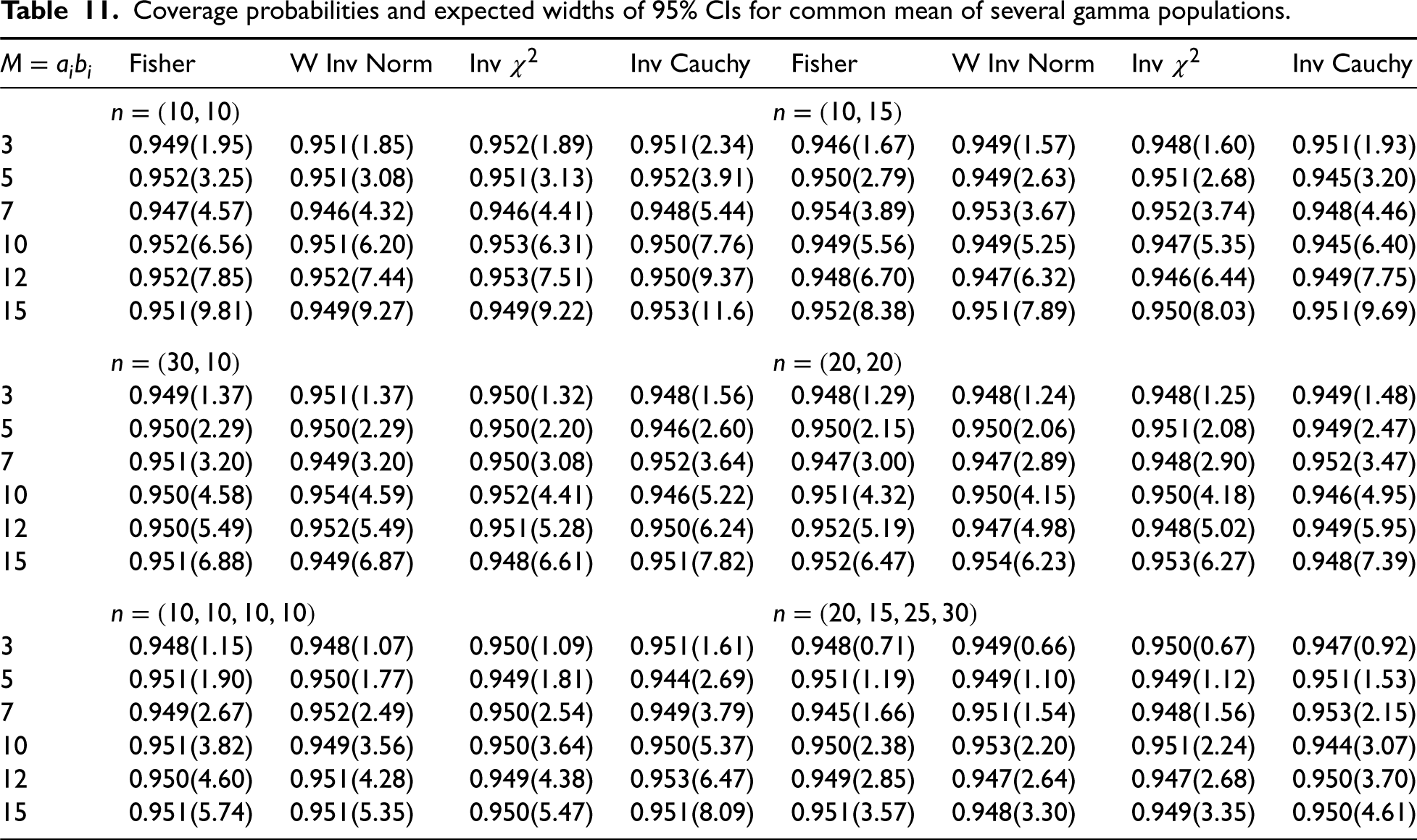
We have carried out some simulation studies to judge the accuracy of the CIs based on Fisher’s combined test, inverse ${\chi }^2$ test, the weighted inverse normal test and the inverse Cauchy test. Other fiducial CIs by Krishnamoorthy and Wang ³⁷ and Yan ⁸ are approximate and they are in general inferior to other CIs based on combined tests. So these CIs are not included in our simulation studies here, but available in Murshed’s ³⁰ Ph.D. dissertation. The simulation estimates of the coverage probabilities and expected widths of 95% CIs are reported in Table 11 for some sample sizes ranging from small to moderately large. As the MLRT based on a single sample is highly accurate even for small samples, the combined tests based on them are also highly accurate in terms of coverage probability. All the CIs based on combined tests control the coverage probabilities very close to the nominal level 0.95 for all cases. Comparison of expected widths clearly indicates that the inverse Cauchy method produced wider CIs for all cases considered in the table. Fisher’s CIs are slightly wider than the other two CIs based on inverse normal and inverse ${\chi }^2$ combined tests in most cases, and it is slightly better than the CIs based on weighted inverse normal test in some cases; see the results for $n=(20,12,8,6)$ in Table 11. There is no clear-cut winner between the CIs based on the inverse ${\chi }^2$ test and the weighted inverse normal test. These two comparable CIs with higher precisions are preferable among all CIs.

Table 11.

Coverage probabilities and expected widths of 95% CIs for common mean of several gamma populations.

$M=a_i{b}_i$	Fisher	W Inv Norm	Inv ${\chi }^2$	Inv Cauchy	Fisher	W Inv Norm	Inv ${\chi }^2$	Inv Cauchy
	$n=(10,10)$				$n=(10,15)$
3	0.949(1.95)	0.951(1.85)	0.952(1.89)	0.951(2.34)	0.946(1.67)	0.949(1.57)	0.948(1.60)	0.951(1.93)
5	0.952(3.25)	0.951(3.08)	0.951(3.13)	0.952(3.91)	0.950(2.79)	0.949(2.63)	0.951(2.68)	0.945(3.20)
7	0.947(4.57)	0.946(4.32)	0.946(4.41)	0.948(5.44)	0.954(3.89)	0.953(3.67)	0.952(3.74)	0.948(4.46)
10	0.952(6.56)	0.951(6.20)	0.953(6.31)	0.950(7.76)	0.949(5.56)	0.949(5.25)	0.947(5.35)	0.945(6.40)
12	0.952(7.85)	0.952(7.44)	0.953(7.51)	0.950(9.37)	0.948(6.70)	0.947(6.32)	0.946(6.44)	0.949(7.75)
15	0.951(9.81)	0.949(9.27)	0.949(9.22)	0.953(11.6)	0.952(8.38)	0.951(7.89)	0.950(8.03)	0.951(9.69)
	$n=(30,10)$				$n=(20,20)$
3	0.949(1.37)	0.951(1.37)	0.950(1.32)	0.948(1.56)	0.948(1.29)	0.948(1.24)	0.948(1.25)	0.949(1.48)
5	0.950(2.29)	0.950(2.29)	0.950(2.20)	0.946(2.60)	0.950(2.15)	0.950(2.06)	0.951(2.08)	0.949(2.47)
7	0.951(3.20)	0.949(3.20)	0.950(3.08)	0.952(3.64)	0.947(3.00)	0.947(2.89)	0.948(2.90)	0.952(3.47)
10	0.950(4.58)	0.954(4.59)	0.952(4.41)	0.946(5.22)	0.951(4.32)	0.950(4.15)	0.950(4.18)	0.946(4.95)
12	0.950(5.49)	0.952(5.49)	0.951(5.28)	0.950(6.24)	0.952(5.19)	0.947(4.98)	0.948(5.02)	0.949(5.95)
15	0.951(6.88)	0.949(6.87)	0.948(6.61)	0.951(7.82)	0.952(6.47)	0.954(6.23)	0.953(6.27)	0.948(7.39)
	$n=(10,10,10,10)$				$n=(20,15,25,30)$
3	0.948(1.15)	0.948(1.07)	0.950(1.09)	0.951(1.61)	0.948(0.71)	0.949(0.66)	0.950(0.67)	0.947(0.92)
5	0.951(1.90)	0.950(1.77)	0.949(1.81)	0.944(2.69)	0.951(1.19)	0.949(1.10)	0.949(1.12)	0.951(1.53)
7	0.949(2.67)	0.952(2.49)	0.950(2.54)	0.949(3.79)	0.945(1.66)	0.951(1.54)	0.948(1.56)	0.953(2.15)
10	0.951(3.82)	0.949(3.56)	0.950(3.64)	0.950(5.37)	0.950(2.38)	0.953(2.20)	0.951(2.24)	0.944(3.07)
12	0.950(4.60)	0.951(4.28)	0.949(4.38)	0.953(6.47)	0.949(2.85)	0.947(2.64)	0.947(2.68)	0.950(3.70)
15	0.951(5.74)	0.951(5.35)	0.950(5.47)	0.951(8.09)	0.951(3.57)	0.948(3.30)	0.949(3.35)	0.950(4.61)

7.3. Gamma distribution: An example

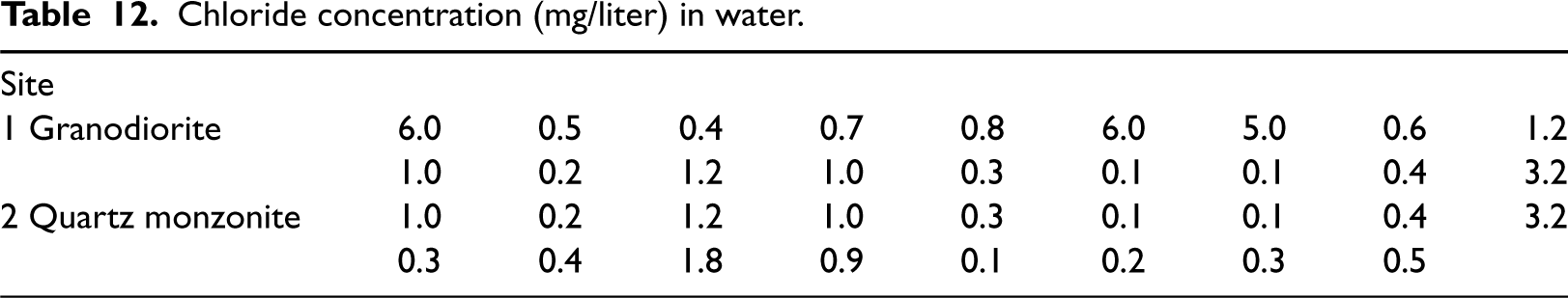
The data in the following Table 12 are measurements of chloride concentration in spring water samples from two types of rocks in Sierra Nevada, California and Nevada. The data are reported in Feth et al. ³⁸ Gamma distributions are routinely used to analyze such pollution measurement data. Yan ⁸ has used the data to find a CI for the common mean concentrations in both sites. The MLEs are ${\hat{a}}_1=0.83564$ , ${\hat{b}}_1=1.9081$ , ${\hat{a}}_2=1.1359$ and ${\hat{b}}_2=0.62143$ .

Table 12.

Chloride concentration (mg/liter) in water.

Site
1 Granodiorite	6.0	0.5	0.4	0.7	0.8	6.0	5.0	0.6	1.2
	1.0	0.2	1.2	1.0	0.3	0.1	0.1	0.4	3.2
2 Quartz monzonite	1.0	0.2	1.2	1.0	0.3	0.1	0.1	0.4	3.2
	0.3	0.4	1.8	0.9	0.1	0.2	0.3	0.5

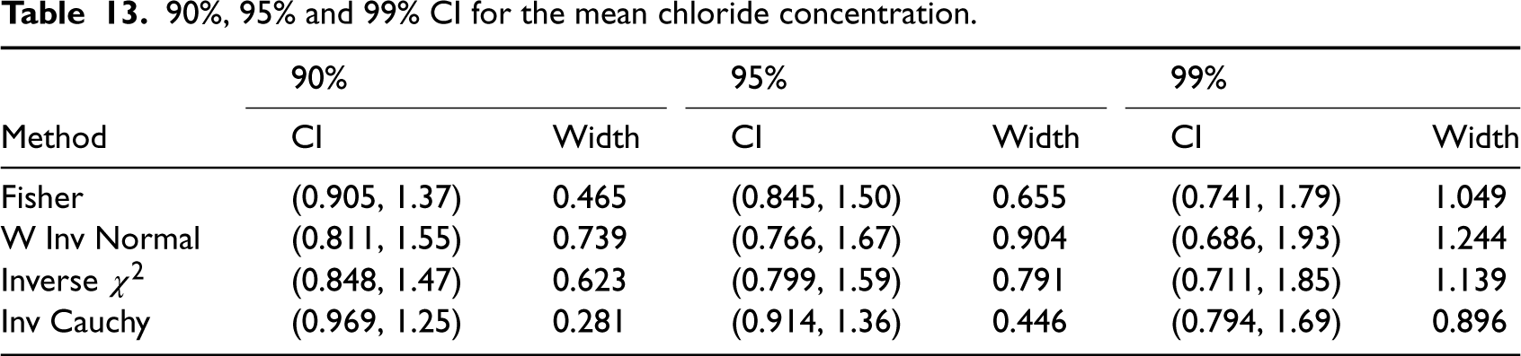
We computed confidence intervals for the common mean of chloride concentrations in both sites using all methods and reported them in Table 13. For this example, the inverse Cauchy CIs are the shortest for all three nominal confidence levels. The 95% generalized CI reported in Yan ⁸ is (0.524, 1.366) with width 0.842, which is somewhat different from other 95% CIs in Table 13. We used the R function CI.common.mean.gamma(n, xb, xd, sq, cl,method) provided in the supplementary file to compute the CIs based on the Fisher, inverse normal, inverse chi-square and the inverse Cauchy methods.

Table 13.

90%, 95% and 99% CI for the mean chloride concentration.

	90%		95%		99%
Method	CI	Width	CI	Width	CI	Width
Fisher	(0.905, 1.37)	0.465	(0.845, 1.50)	0.655	(0.741, 1.79)	1.049
W Inv Normal	(0.811, 1.55)	0.739	(0.766, 1.67)	0.904	(0.686, 1.93)	1.244
Inverse ${\chi }^2$	(0.848, 1.47)	0.623	(0.799, 1.59)	0.791	(0.711, 1.85)	1.139
Inv Cauchy	(0.969, 1.25)	0.281	(0.914, 1.36)	0.446	(0.794, 1.69)	0.896

8. Concluding remarks

A typical method of finding a CI for a parameter of interest is inverting a test for the parameter. If the test is exact, in the sense that the null distribution of the test statistic does not depend on any unknown parameter, then the CI that is obtained by inverting the test is also exact. This well-known approach to find CIs based on data from different independent resources was seldom investigated in the present context. In this article, we investigated such method and shown that efficient exact CIs for a common parameter of interest can be readily obtained by inverting a combined test. Eventhough there are a few exact combined tests available in the literature, the CIs based on them were seldom utilized. The methods that we considered in this article are conceptually simple, but they involve numerical computations. To help practitioners and other researchers, we provided R code in a supplementary file that can be used in a straightforward manner to compute the CIs based on the Fisher, inverse chi-square, and weighted inverse normal methods.

We also investigated (not reported here) robustness of the interval estimation procedures. For example, as both lognormal and gamma distributions are used to model positive right-skewed data, we investigated numerically if the CIs for a common mean of several gamma populations can be used to estimate a common mean of several lognormal populations. Our investigation indicated that such gamma-based CIs are too liberal when they are used for lognormal populations. In general, the combined tests and the method of finding CIs are valid only when the model assumptions are satisfied. This is because the individual tests (such as the $t$ -tests for normal and the LRTs for the gamma and log-normal) that were used to combine are valid only for the assumed models.

It should be clear that the proposed method of finding a CI for a common parameter of interest can be readily applied to practical problems where an exact test or highly accurate test such as the MLRT based on a single sample is available. For example, our approach can be readily extended to find the confidence region of a common mean vector of several multivariate normal distributions. We are currently extending the proposed approach to the case of multivariate normal and plan to publish the work elsewhere.

Supplemental Material

sj-txt-1-smm-10.1177_09622802231217644 - Supplemental material for Confidence estimation based on data from independent studies

Supplemental material, sj-txt-1-smm-10.1177_09622802231217644 for Confidence estimation based on data from independent studies by Kalimuthu Krishnamoorthy and Md Monzur Murshed in Statistical Methods in Medical Research