Marginal structural models with latent class growth analysis of treatment trajectories: Statins for primary prevention among older adults

Abstract

Latent class growth analysis is increasingly proposed as a solution to summarize the observed longitudinal treatment into a few distinct groups. When latent class growth analysis is combined with standard approaches like Cox proportional hazards models, confounding bias is not properly addressed because of time-varying covariates that have a double role of confounders and mediators. We propose to use latent class growth analysis to classify individuals into a few latent classes based on their medication adherence pattern, then choose a working marginal structural model that relates the outcome to these groups. The parameter of interest is defined as a projection of the true marginal structural model onto the chosen working model. Simulation studies are used to illustrate our approach and compare it with unadjusted, baseline covariates adjusted, time-varying covariates adjusted, and inverse probability of trajectory groups weighted adjusted models. Our proposed approach yielded estimators with little or no bias and appropriate coverage of confidence intervals in these simulations. We applied our latent class growth analysis and marginal structural model approach to a database comprising information on 52,790 individuals from the province of Quebec, Canada, aged more than 65 and who were statin initiators to estimate the effect of statin-usage trajectories on a first cardiovascular event.

1. Introduction

Cardiovascular disease (CVD) is the leading cause of death worldwide. ¹ One of the most commonly used treatments to prevent CVDs is $\beta$ -hydroxy $\beta$ -methylglutaryl-coenzyme A reductase inhibitors, statins. ² Several randomized controlled trials (RCTs) have shown the efficacy of statins to prevent a first CVD event, that is, for primary prevention. ³ However, a gap in knowledge remains concerning the efficacy of statins for primary prevention in older adults (i.e. adults aged 65 or older) as they are often excluded from RCTs. ⁴ Also, treatment adherence, defined as the patient’s compliance with the physician’s recommendations, ⁵ is often poorer in real-world situations, which translates in less benefits than in RCTs. ⁶ Analysis of observational data could add crucial information on the benefits of actual patterns of statin use (i.e. adherence over time) among older adults. However, the number of possible unique treatment trajectories increases exponentially with the length of the follow-up in longitudinal studies.

Latent class growth analysis (LCGA), or group-based trajectory models, are increasingly proposed as a solution to summarize the observed trajectories in a few distinct groups. ⁷ LCGA defines homogeneous subgroups of individuals with respect to their patterns of adherence over time. ⁸ Using real-world data, Franklin et al. ⁷ applied LCGA to classify patients who initiated a statin treatment according to their pattern of long-term adherence. The authors compared LCGA with traditional measures of medication adherence, such as the proportion of days covered or medication possession ratio, and concluded that LCGA is a better method to summarize adherence as it is more informative of the various observed patterns of treatment use over time.

While LCGA is a promising approach for summarizing the observed treatment trajectories in a few trajectory groups, estimating the effect of the trajectory groups using observational data requires adequate adjustment for potential time-dependent confounders. Franklin et al. ⁹ estimated the association between statin adherence trajectory groups and CVD events using a two-step approach, wherein LCGA was used in a first step to create trajectory groups and then used as an exposure in a Cox model adjusted for baseline covariates in a second step. Unfortunately, this approach may not adequately control confounding bias because of treatment-confounder feedback. Indeed, time-dependent confounders can be affected by past treatment adherence, ¹⁰ and thus have a double-role of confounders and mediators. In such situations, standard approaches, including covariate adjustment in an outcome regression model, fail to control confounding adequately. ¹⁰ Estimators of the parameters of marginal structural models (MSMs) such as inverse probability weighting (IPW) are well-known in the causal inference literature for their ability to deal appropriately with time-varying covariates and time-varying treatment. ¹¹

MSMs are a class of causal models that model the expected counterfactual outcome as a function of treatment trajectories. However, modeling the expected counterfactual outcome as a function of all possible treatment trajectories might lead to non- or partial-identifiability of standard MSM parameters. A common alternative is to model the outcome as a function of the cumulative number of periods of treatment adherence. This approach lacks flexibility since it assumes a linear relationship between cumulative treatment adherence and outcome. A flexible Cox MSM with a weighted cumulative exposure was proposed by Xiao et al. ¹² The weighted cumulative exposure is estimated with splines allowing for a data-driven specification of the relationship between the expected counterfactual outcome and the observed treatment trajectory. While this alternative is flexible, it does not directly measure the impact of adherence, instead focusing on estimating how the effect of the treatment varies in time, and summarizing this information as a weighted sum. An attempt to combine trajectory analysis with MSM was proposed by Lim et al. who used the stabilized inverse of the probability of the trajectory groups as weights. ¹³ To define trajectory groups, they used a sequence analysis to group similar profiles. ¹³ We expect such an estimation method to be inappropriate to correctly control for time-varying confounders.

In this article, we propose a formal theoretical framework to combine LCGA and MSMs. We first use a finite mixture modeling approach (LCGA) to cluster the observed treatment trajectories into several latent classes or trajectory groups. We propose considering the LCGA as a dimension reduction technique that allows clustering similar individual treatment trajectories in trajectory groups, even when true latent trajectory groups do not exist. In a second step, we define the causal parameter of interest as a projection of the true nonparametric MSM on a working parametric MSM relating the mean counterfactual outcome to the trajectory groups found in the first step. ¹⁴ Hence, we alleviate the burden of assuming a correctly specified model (i.e. the working model is not assumed to be the true model). We propose an IPW estimator of this parameter. Inferences concerning the effect of the trajectory groups are conditional on the clustering solution found in the first step. As such, the trajectory groups are considered as fixed in the outcome model rather than random and inferences can proceed ignoring the clustering step. Indeed, as multiple authors have previously argued, clustering performed according to explanatory variables only (i.e. not using information on the outcome) do not invalidate inferences.^15–17 To provide further justification regarding the validity of the LCGA–MSM, we explicitely derived the expression of the IPW estimating function and its variance. Several studies had for objective of estimating the effects of exposure trajectories, such as the effect of medication adherence trajectories or incarceration trajectories, and could benefit from the approach we propose.^13,9 As far as we know, such a combination of MSMs with LCGA that allows for the control of time-varying confounders has never been investigated. In the remainder, we present the modeling framework (notation, causal model, mixture model, and estimation approach) followed by a simulation study to illustrate and investigate the finite-sample properties of our proposal. We also present an application to real data where we estimate the effect of long-term adherence to statins for primary prevention of CVD among older adults before ending the paper with some recommendations for the practical application of our proposed approach.

2. Notation and nonparametric marginal structural model definition

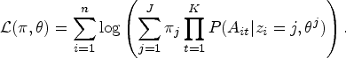
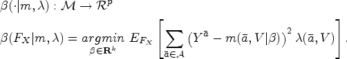
In the following, we use capital letters to represent random variables and corresponding lower case letters to represent observed or fixed values these variables take. Consider a longitudinal study where $t=1,\dots ,K$ is the follow-up time and in which the observed data structure is $\mathcal{O}=\{Y,{\overline{A}}_t,{\overline{L}}_t\}$ . Let ${\overline{A}}_t=(A_1,A_2,\dots ,A_t)$ be the treatment trajectory up to time $t$ . Similarly, ${\overline{L}}_t=(L_1,L_2,\dots L_t)$ is the covariates’ history up to time $t$ . As a notational shortcut, we define $\overline{A}\equiv {\overline{A}}_K$ and $\overline{L}\equiv {\overline{L}}_K$ . Let $Y$ be the observed outcome at the end of the follow-up. We denote by $Y^{\overline{a}}$ the counterfactual outcome under a specific treatment trajectory, that is, the outcome that would have been observed had the treatment trajectory been $\overline{a}$ , possibly contrary to fact. Similarly, ${\overline{L}}^{\overline{a}}$ denotes a counterfactual covariate process. We denote by $F_X$ the unknown joint distribution of all possible counterfactual variables $X=({\overline{L}}^{\overline{a}},Y^{\overline{a}}:\overline{a}\in \mathcal{A})$ where $\mathcal{A}$ is the set of all possible values of $\overline{a}$ . We denote by $P_{F_X}$ the distribution of the observed data from which $i=1,\dots ,n$ independent and identically distributed observations are randomly drawn. We consider the following nonparametric form of an MSM, where $m^{*}$ is the true MSM and $V$ is a (possibly empty) subset of the baseline covariates, $V\subseteq L_1$ :

$$E_{F_X}(Y^{\overline{a}}|V)=m^{*}(\overline{a},V).$$

(1)

Equation (1) represents a model where the distribution of all possible counterfactual variables, $F_X$ , is left unknown. Thus, we do not make the assumption of a correctly specified model as would be the case when considering a parametric MSM. The nonparametric identification of model (1) from the observed data can be achieved under the following causal assumptions ¹⁴ : (1) sequential conditional exchangeability, (2) no interference between subjects, (3) consistency, and (4) positivity. Assumption 1 indicates that, conditional on the history of treatment up to time $t-1$ and the history of the covariates up to time $t$ , there are no unmeasured confounders, ¹⁸ that is $Y^{\overline{a}}\mathbf{\perp }\mathbf{\perp }{A}_t|{\overline{A}}_{t-1},{\overline{L}}_t$ . Assumption 2 means that the potential outcome of a given individual is not affected by the treatment of the other subjects. Assumption 3 means that, given the observed treatment trajectory, the observed outcome and the potential outcome under that given trajectory are the same, formally if $\overline{A}=\overline{a}$ then $Y^{\overline{a}}=Y$ . Assumption 4 requires that for each level $({\overline{a}}_t,{\overline{l}}_t)$ , $P(A_t=a_t|{\overline{A}}_{t-1}={\overline{a}}_{t-1},{\overline{L}}_t={\overline{l}}_t)>0$ . In other words, in each stratum defined by previous treatment and covariates, there is a non-zero probability to find both exposed and unexposed individuals at time $t$ . These assumptions are essential to identify the parameters of the LCGA–MSM we propose later. Under these assumptions, we have:

$${\mathbb{E}}_{F_X}\left(Y^{\overline{a}}\right)={\int }_{{\mathit{l}}_{\mathbf{1}}}\dots {\int }_{{\mathit{l}}_{\mathit{K}}}\mathbb{E}(Y|{\overline{a}}_K,{\overline{\mathit{l}}}_K)f({\mathit{l}}_{\mathit{K}}|{\mathit{l}}_{\mathit{K}\mathbf{-}\mathbf{1}},{\overline{a}}_{K-1})\mu ({\mathit{L}}_{\mathit{K}}),\dots ,f({\mathit{l}}_{\mathbf{1}})\mu ({\mathit{L}}_{\mathbf{1}}),$$

(2)

where $f({\mathit{l}}_{\mathit{K}}|{\mathit{l}}_{\mathit{K}\mathbf{-}\mathbf{1}},{\overline{a}}_{K-1}),\dots ,f({\mathit{l}}_{\mathbf{1}})$ are the densities of ${\overline{\mathit{L}}}_{\mathit{t}}$ relative to appropriate measures $\mu ({\mathit{L}}_{\mathit{t}}),t=1,\dots ,K$ , respectively. ¹⁹

Due to the curse of dimensionality, equation (2) is rarely solvable with finite sample data. As mentioned in the “Introduction” section, one challenge is related to the number of treatment trajectories. In the next two sections, we introduce our LCGA–MSM as a solution to this specific challenge.

3. Summarizing treatment trajectories with latent class growth models

The first step of our LCGA–MSM proposal consists of summarizing treatment trajectories with a LCGA. As will be seen, LCGA assumes the existence of true latent groups that explain the observed trajectories. We regard this as a working assumption and instead use LCGA as a convenient statistical technique for summarizing the observed trajectories in a few distinct groups. In other words, our LCGA–MSM approach does not rely on the existence of true latent groups and instead uses the LCGA to create groups of individuals with similar observed trajectories. Remark that Nagin ⁸ proposes a similar perspective to LCGA, where the groups are seen as an approximation to the underlying truth.

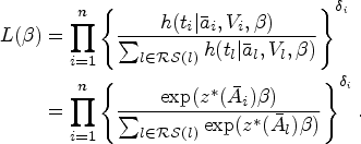
Let $z_i$ denote the latent group-membership or trajectory group for the $i$ ^th individual estimated from the individual’s observed treatment ${\overline{A}}_i,i=1,\dots ,n$ . We denote by ${\pi }_j$ the probability that an individual belongs to the $j$ ^th trajectory group in the population, $j=1,\dots ,J$ , where $J$ is the total number of groups with the constraints ${\pi }_j\ge 0$ and $\sum _{j=1}^J{\pi }_j=1$ . In LCGA, each trajectory group is often described by a group-specific polynomial function of time. For example, if a quadratic relation was assumed for the $j$ ^th group, we could use the regression model $logit(P(A_{it}=1|z_i=j))={\theta }_0^j+{\theta }_1^{j}t+{\theta }_2^j{t}^2$ , where the parameters ${\theta }^j,j=1,\dots ,J$ , describe the treatment trajectory over time for the $j$ ^th group. This specification implies that the following mixture model is the marginal probability of the treatment trajectories $P({\overline{A}}_i)$ :

$$P({\overline{A}}_i)=\sum _{j=1}^J{\pi }_j\prod _{t=1}^{K}P(A_{it}|z_i=j).$$

(3)

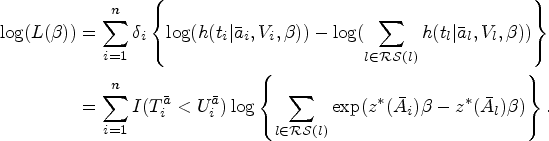
Model (3) relies on the local independence assumption, that is, treatment at different time-points $A_{i1},\dots ,A_{iK}$ are assumed to be mutually independent conditional on group membership ²⁰ : $A_{it}\perp \perp A_{i{t}^{{}^{\prime }}}|z_i=j,\text{for all}t\ne t^{{}^{\prime }},j=1,\dots ,J$ . We regard this assumption as a working assumption in our LCGA–MSM approach. Under the local independence assumption, the log-likelihood of the $n$ observations is given by:

$$\mathcal{L}(\pi ,\theta )=\sum _{i=1}^n\log (\sum _{j=1}^J{\pi }_j\prod _{t=1}^{K}P(A_{it}|z_i=j,{\theta }^j)).$$

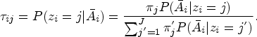
We denote by ${\tau }_{ij}=P(z_i=j|{\overline{A}}_i)$ the $i$ ^th individual conditional (“posterior”) probability of membership in group $j$ ,

$${\tau }_{ij}=P(z_i=j|{\overline{A}}_i)={\displaystyle \frac{{\pi }_{j}P({\overline{A}}_i|z_i=j)}{\sum _{j^{{}^{\prime }}=1}^J{\pi }_j^{{}^{\prime }}P({\overline{A}}_i|z_i=j^{{}^{\prime }})}}.$$

These probabilities are computed post-model fitting and are used to assign subjects into a trajectory group, usually based on their largest value. ⁸ Therefore, we can formally define the assigned trajectory groups as $z_i={argmax}_{j=1,\dots ,J}{\tau }_{ij}$ .

In Figure 1, we present a global overview of the LCGA approach. From the $n\times K$ matrix of the observed treatment trajectories, we determine the $n\times J$ matrix of individual conditional probabilities which in turn yields the $n\times 1$ vector of trajectory groups.

Figure 1.

Summarizing the observed treatment trajectories into $J$ trajectory groups with latent class growth analysis (LCGA). The $n\times K$ matrix represents the observed treatment values for all $n$ individuals over the $K$ follow-up times. The $n\times J$ matrix represents the conditional probabilities of membership to group $j$ for the $n$ individuals. The $n\times 1$ vector represents the assigned trajectory groups of the $n$ individuals. The formulas above the arrows indicate how to obtain these matrices.

We note that the local independence assumption of LCGA is unlikely to hold in the presence of time-dependent confounding. Indeed, time-dependent confounding is susceptible to create a complex dependence structure between treatments at different time-points. As argued previously, if this assumption does not hold, LCGA can still be regarded as a convenient statistical technique to summarize treatment trajectories into trajectory groups. However, it is then crucial to assess that the chosen LCGA model provides a good approximation to the observed treatment trajectories. It is common to use various statistical indices to select the number of groups $J$ , the polynomial order of the trajectory groups, and to assess the fit of the model to the data. The approach proposed by Nagin consists in first comparing models with different number of groups and choosing the one that minimizes the Bayesian information criterion (BIC), fixing the polynomial order of the groups. ⁸ Other considerations, such as the interpretability of the selected model and ensuring that a sufficient number of subjects (e.g. $\ge$ 250 subjects) are present in each group, are also employed together with the BIC to select the number of groups. ²¹ Once the number of groups is chosen, models with different polynomial orders are compared to select the one that minimizes the BIC. The entropy information criterion (EIC) is recommended to assess how well the clusters are separated. ²² Nagin proposes other fit indices, including the average posterior probability of assignment and the odds of correct classification. ⁸

A general framework for fitting LCGA is implemented in the R package FlexMix which is based on an expectation-maximization (EM) algorithm. ²³ Note that a slightly different expression of the log-likelihood is used in this EM algorithm. ²⁴

4. Defining the causal parameter of interest

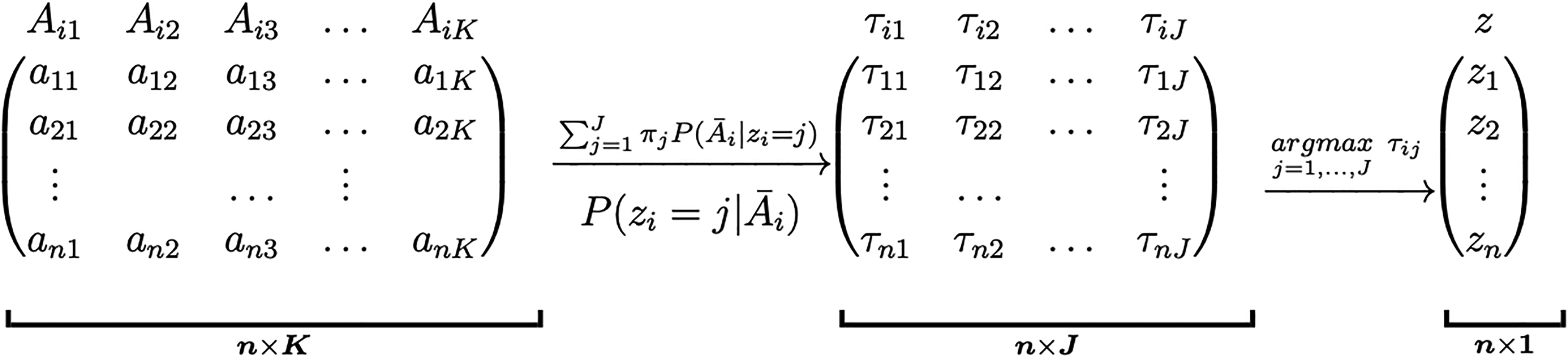
Once the observed treatment trajectories are summarized using LCGA, the next step of our LCGA-MSM approach is to formally define the causal effect of interest. We propose in a second step to approximate the nonparametric MSM $m^{*}(\overline{a},V)$ for all $\overline{a}\in \mathcal{A}$ with a working MSM that is a function of the identified trajectory groups. An important feature of our LCGA-MSM approach is thus that it is not assumed that the identified groups represent some underlying truth. Instead, the groups are seen as an approximation to the truth that facilitates practical interpretation and that alleviates the challenge of estimating the parameters of a saturated MSM. Intuitively, the parameter of interest can be conceptualized as follows: if we were to conduct a randomized trial with $2^K$ groups consisting of the $2^K$ possible individual treatment trajectories, and then cluster the treatment groups according to the $J$ trajectory groups found in the first step, how would the mean outcome differ between clusters? It is worth recalling once more that the first step does not involve the response variable $Y$ ; as we can see in Figure 2, the follow-up period of the treatment and the outcome are distinct. For now, we assume that the treatment follow-up period is complete for all individuals. We propose a causal parameter of interest that accounts for the possibility of incomplete treatment follow-up at the end of the currentsection.

Figure 2.

Illustration of the two steps latent class growth analysis and marginal structural model (LCGA–MSM) approach with a follow-up period of 60 months.

Following a notation similar to Neugebauer and van der Laan, ¹⁴ we denote by ${\mathcal{M}}^{*}$ the infinite-dimensional space of all possible functions $m^{*}$ relating the counterfactual expectation with the treatment trajectories and baseline covariates $V$ as in equation (1). We define $\mathcal{M}$ a subset of ${\mathcal{M}}^{\mathcal{\ast }}$ , consisting of all the family of functions $m$ that the user is interested in using to characterize how the expectations of the counterfactual outcomes are related to the treatment trajectories and baseline covariates $V$ (i.e. the working model). Let $z_i$ be the trajectory group assigned to subject $i$ as defined previously and $z^{*}(\overline{a})=(z_1^{*}(\overline{a}),\dots ,z_J^{*}(\overline{a}))$ dummy variables indicating whether the individual trajectory $\overline{a}$ is clustered in each of the trajectory group. Our LCGA–MSM approach entails specifying $\mathcal{M}=\{m(z^{*}(\overline{a}),V|\beta ):\beta \in {\mathcal{R}}^p\}$ , where $p$ is the number of parameters in $m(z^{*},V|\beta )$ . One example of a working LCGA–MSM is: $\mathbb{E}[Y^{\overline{a}}]={\beta }_0+{\beta }_1{z}_1^{*}(\overline{a})+\cdots +{\beta }_{J-1}{z}_{J-1}^{*}(\overline{a})$ . The model could feature additional parameters for covariates $V$ and for interaction terms between $z^{*}(\overline{a})$ and $V$ if effect modification is relevant. Remark that if $V=\mathrm{\varnothing }$ and $J=2^K$ , then $\mathcal{M}={\mathcal{M}}^{*}$ . Indeed, the number of trajectory groups would then correspond to the total number of possible trajectories, and the working model would besaturated.

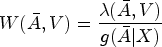
Our causal parameter of interest is defined as a projection of the true nonparametric MSM $m^{*}$ on the working model $m$ . This projection is notably characterized by a weight function $\lambda (\overline{a},V)$ that determines, for all $(\overline{a},v)\in \mathcal{A}\times {\mathcal{S}}_V$ , where ${\mathcal{S}}_V$ is the set of all possible values of $V$ (its support), how well the working MSM $m$ should approximate the true MSM $m^{*}$ relative to other values of $(\overline{a},v)$ . More formally:

$$\begin{array}{rl}& \beta (\cdot |m,\lambda ):{\mathcal{M}}^{\mathcal{\ast }}\to {\mathcal{R}}^p\\ & {\beta }_{m,\lambda }=\underset{\beta \in {\mathbf{R}}^p}{argmin}\Vert m^{*}-m(z^{*}(\overline{a}),V|\beta ){\Vert }_{\lambda (\overline{a},V)}.\end{array}$$

(4)

In other words, $\beta \equiv {\beta }_{m,\lambda }=\beta (F_X|m,\lambda )$ is chosen according to $\lambda$ to minimize the “distance” between the true model $m^{*}$ and the working model $m$ according to a given loss-function $||\cdot |{|}_{\lambda }$ . Note that the trajectory groups $z$ are only a function of the time-varying treatment ( $\overline{a}$ ) in the LCGA approach. Therefore, we can write $m(z^{*}(\overline{a}),V|\beta )\equiv m(\overline{a},V|\beta )$ . When $Y$ is part of an exponential family, a natural choice for the loss function is derived from its log-likelihood. For example, when the outcome $Y$ is continuous, a weighted $L_2$ loss function is commonly used:

$$\begin{array}{rl}& \beta (\cdot |m,\lambda ):\mathcal{M}\to {\mathcal{R}}^p\\ & \beta (F_X|m,\lambda )=\underset{\beta \in {\mathbf{R}}^k}{argmin}{E}_{F_X}[\sum _{\overline{a}\in \mathcal{A}}{(Y^{\overline{a}}-m(\overline{a},V|\beta ))}^2\lambda (\overline{a},V)].\end{array}$$

The choice of $\lambda (\overline{a},V)$ depends on the modeling goals. Common choices notably include $\lambda (\overline{a},V)=1$ , which would be suitable if it is desired to get a global summary of the nonparametric causal model, and $\lambda (\overline{a},V)=\prod _{t=1}^{K}P(A_t|{\overline{A}}_{t-1},V)$ which gives more weights to trajectories that are frequently observed.

In the presence of incomplete treatment follow-up, the treatment regime $\overline{A}$ can be characterized as a bivariate variable $\overline{A}=(\overline{A}(1)=\overline{a}(1),\overline{A}(2)=0)$ , in which $\overline{A}(2)=0$ represents an intervention that prevents censoring or events from occurring during the treatment follow-up period. The same identifying assumptions (i.e. exchangeability, no interference, consistency, and positivity) are required, but now relative to this bivariate treatment variable. From a practical perspective, the proposed parameter quantifies how the average outcome differs according to trajectory groups in a hypothetical randomized experiment without loss to follow-up and without any outcome events during the treatment follow-up.

4.1. Time-to-event analysis

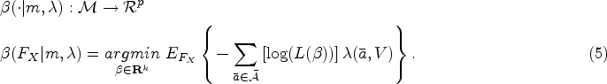
When $Y$ is a time-to-event outcome, we define our working causal model as a Cox proportional hazards MSM, where $h_0(t)$ is the baseline hazard function:

$$h^{\overline{a}}(t)=h_0(t)exp({\beta }_1{z}_1^{*}(\overline{a})+\cdots +{\beta }_{J-1}{z}_{J-1}^{*}(\overline{a})).$$

We define $E(T^{\overline{a}}|V,\beta )={\int }_t{S}^{\overline{a}}(t)={\int }_{t}exp(-H^{\overline{a}}(t))={\int }_{t}exp(-{\int }_k^{t}h(t|\overline{a},V,\beta ))\equiv m(\overline{a},V|\beta )$ . As in our illustration, the loss function can be defined from the negative partial log-likelihood. Let $Y^{\overline{a}}$ denote the minimum between the counterfactual survival time $T^{\overline{a}}$ and the censoring time denoted by $U^{\overline{a}}$ . The indicator for the event is designated by $\delta$ where $\delta =1$ if $T^{\overline{a}}<U^{\overline{a}}$ and 0 otherwise. Also let $\mathcal{R}\mathcal{S}(l{)}_{\overline{a}}=\{i=1,\dots ,n:T^{\overline{a}}>l\}$ designate the set of individuals at risk at time $l$ under the counterfactual intervention $\overline{a}$ . We define the partial likelihood as a function of the trajectory groups as follows:

$$\begin{array}{rl}L(\beta )& =\prod _{i=1}^n{\left\{{\displaystyle \frac{h(t_i|{\overline{a}}_i,V_i,\beta )}{\sum _{l\in \mathcal{R}\mathcal{S}(l)}h(t_l|{\overline{a}}_l,V_l,\beta )}}\right\}}^{{\delta }_i}\\ & =\prod _{i=1}^n{\left\{{\displaystyle \frac{\exp (z^{*}({\overline{A}}_i)\beta )}{\sum _{l\in \mathcal{R}\mathcal{S}(l)}\exp (z^{*}({\overline{A}}_l)\beta )}}\right\}}^{{\delta }_i}.\end{array}$$

Thus, the partial log-likelihood is given by

$$\begin{array}{rl}\log (L(\beta ))& =\sum _{i=1}^n{\delta }_i\{\log (h(t_i|{\overline{a}}_i,V_i,\beta ))-\log (\sum _{l\in \mathcal{R}\mathcal{S}(l)}h(t_l|{\overline{a}}_l,V_l,\beta ))\}\\ & =\sum _{i=1}^{n}I(T_i^{\overline{a}}<U_i^{\overline{a}})\log \{\sum _{l\in \mathcal{R}\mathcal{S}(l)}\exp (z^{*}({\overline{A}}_i)\beta -z^{*}({\overline{A}}_l)\beta )\}.\end{array}$$

We define our parameter of interest $\beta$ as follows:

$$\begin{array}{rl}& \beta (\cdot |m,\lambda ):\mathcal{M}\to {\mathcal{R}}^p\\ & \beta (F_X|m,\lambda )=\underset{\beta \in {\mathbf{R}}^k}{argmin}{E}_{F_X}\{\mathbf{-}\sum _{\overline{a}\in \overline{\mathcal{A}}}[\log (L(\beta ))]\lambda (\overline{a},V)\}.\end{array}$$

(5)

5. Estimation of the parameter of the LCGA–MSM

We now describe how the parameter $\beta$ of our LCGA–MSM can be estimated from the observed data. Because, the distribution of the trajectory groups $z$ does not depend on the parameter of interest $\beta$ , $z$ is an ancillary statistic.^25,26 Indeed, by construction, the distribution of the groups is only a function of the joint distribution of the treatments $\overline{A}$ and is thus independent of the parameter $\beta$ . Therefore, in the second step of our approach, the trajectory groups are not seen as random but rather as a fixed regressor. ²⁷ In other words, the fact that the trajectories are estimated from the data can be ignored when estimating the parameter of our LCGA–MSM and when estimating the standard error of the estimator and confidence intervals. The simulation results presented in Section 6 also support this claim. However, it should be noted that inferences are conditional on the selected LCGA (see Supplemental Appendix A for more details).

5.1. Inverse probability of treatment weighting

Several approaches exist to estimate the parameters of an MSM with one of the most popular being inverse probability of treatment weighting (IPTW). ¹¹ IPTW mimics a random assignment of the treatment by creating a pseudo-population where the treated and the untreated groups are comparable in terms of the distribution of confounders. In longitudinal settings, IPTW can appropriately adjust for time-varying covariates affected by prior exposure. Following Neugebauer and van der Laan, ¹⁴ the IPTW weights are:

$$W(\overline{A},V)={\displaystyle \frac{\lambda (\overline{A},V)}{g(\overline{A}|X)}}$$

where $g(\overline{A}|X)$ is the treatment mechanism which may depend on the counterfactual data $X$ . However, under the sequential conditional exchangeability assumption, $g(\overline{A}|X)=\prod _{t=1}^{K}P(A_t|{\overline{A}}_{t-1},{\overline{L}}_t)$ . In the literature, stabilized weights (i.e. setting $\lambda (\overline{A},V)=\prod _{t=1}^{K}P(A_t|{\overline{A}}_{t-1},V))$ are largely recommended since they tend to yield less extreme values. ²⁸ In presence of incomplete treatment follow-up, IPCW are additionally used and we have $g(\overline{A}|X)=\prod _{t=1}^{K}P(A_t(1),A_t(2)=0|{\overline{A}}_{t-1}(1),{\overline{A}}_{t-1}(2)=0,{\overline{L}}_t)$ under the sequential conditional exchangeability assumption. Intuitively, IPCW aims to mimic what would have happened had everyone had a complete treatment follow-up by redistributing the weights of people with an incomplete treatment follow-up onto individuals with similar characteristics but with a complete treatment follow-up.

5.2. IPTW estimating function

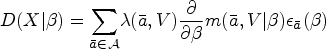
To estimate the parameter of interest ${\beta }_{m,\lambda }$ , we have to define the estimating function of the counterfactual data based on the IPTW. We first differentiate the loss function defined in equation (5) and then we derive from its expression the IPTW estimating function. We denote by $D(X|\beta )$ the first-order derivative of the loss function. Neugebauer and van der Laan ¹⁴ showed that the IPTW estimating function when $Y$ is continuous is given by:

$$D(\mathcal{O}|\beta ,g)={\displaystyle \frac{D(X|\beta )}{g(\overline{A}|X)}}$$

(6)

where the first-order derivative of the $L_2$ loss-function is given by:

$$D(X|\beta )=\sum _{\overline{a}\in \mathcal{A}}\lambda (\overline{a},V){\displaystyle \frac{\mathrm{\partial }}{\mathrm{\partial }\beta }}m(\overline{a},V|\beta ){ϵ}_{\overline{a}}(\beta )$$

with ${ϵ}_{\overline{a}}(\beta )=Y^{\overline{a}}-m(\overline{a},V|\beta )$ is the residual after projecting the nonparametric MSM onto the chosen working model. A well-known property of the IPTW estimating function is its unbiasness at its true parameter which satisfy $E(D(\mathcal{O}|g,\beta ))=0$ see, for example, Neugebauer and van der Laan. ¹⁴ Thus, it can be shown, under the positivity assumption, that the IPTW estimator ${\hat{\beta }}_{m_{IPTW},\lambda }$ of ${\beta }_{m,\lambda }$ is the solution of the estimating equation $\sum _{i=1}^{n}D({\mathcal{O}}_i|g_n,\beta )=0$ , where ${\lambda }_n$ and $g_n$ are estimators of $\lambda$ and $g$ , respectively. To simplify the notation, we define ${\hat{\beta }}_{m_{IPTW},\lambda }\equiv {\hat{\beta }}_n$ . Under the positivity assumption, when $g_n$ and ${\lambda }_n$ are consistent, ${\hat{\beta }}_n$ is consistent and asymptotically linear. ¹⁴ Thus ${\hat{\beta }}_n$ has a unique influence function ²⁹ and can be identified through this. From the expression of the influence function, we determine the asymptotic variance of ${\hat{\beta }}_n$ using Slutsky’s theorem. Thus, we can construct a 95% confidence interval for $\beta$ as ${\hat{\beta }}_{jn}\pm 1.96\times se({\hat{\beta }}_{jn})$ , where $se({\hat{\beta }}_{jn})={\hat{\sum }}_{jn}^{p\times p}$ denotes the $j$ ^th diagonal element of the sandwich variance estimator matrix of dimension $p\times p$ , where $p$ is the number of parameters in $m(\overline{a},V|\beta )$ .

5.3. Implementation of the LCGA–MSM in practice

The LCGA–MSM using the IPW as an estimation method can be summarized in three main steps:

First step: Summarize the observed time-varying treatment by using LCGA. The model for the treatment is a polynomial function of the time.

Second step: Estimate the IPTW using the observed treatment. If some people have an incomplete treatment follow-up, also compute the IPCWs.

Third step: Estimate the parameters of the LCGA–MSM by fitting a model for the outcome according to the trajectory groups using only observations with a complete treatment follow-up, weighting each observation by the IPW and using a robust variance estimator to produce inferences (e.g. confidence intervals).

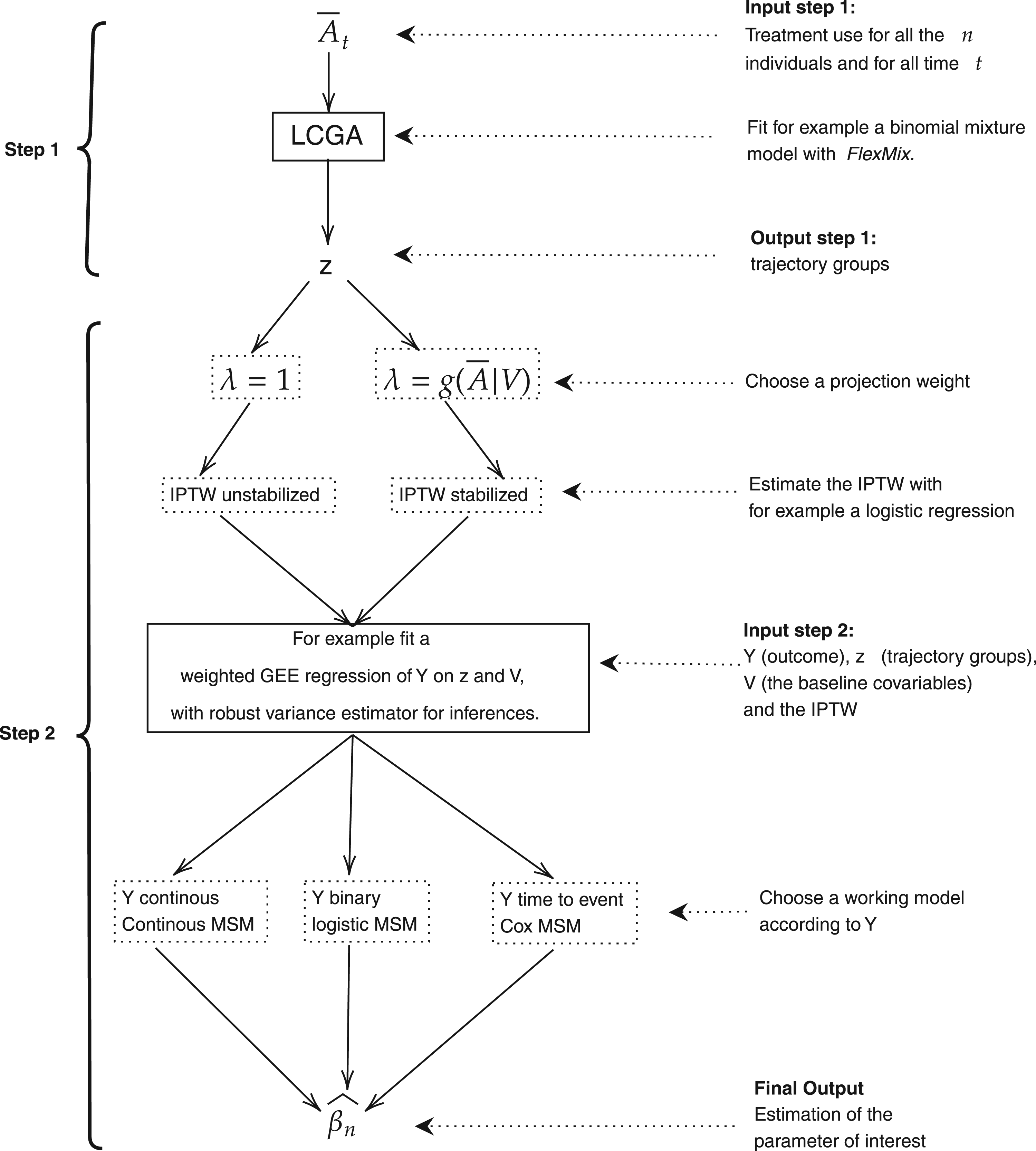
Figure 3 provides a practical template of the estimation approach. It is worth mentioning that beside treatment adherence, LCGA can be used in other contexts.

Figure 3.

Practical template for implementation of the latent class growth analysis and marginal structural model (LCGA–MSM) approach.

In practice, when the distribution of $Y$ is part of the exponential family, the parameters of the working model can be directly estimated using the classical weighted generalized estimating equations (GEEs), with, for example, the function geeglm from the R package geepack. Indeed, under the causal assumptions described previously, the estimating equation (6) are solved by such a weighted GEE procedure. When $Y$ is a time-to-event outcome, a weighted Cox model can be fitted using the R package survival. A simple practical solution for inference is to use the sandwich variance estimator of the GEE routine or of the Cox model, which treats the weights as known and results in conservative statistical inferences. ³⁰

We note that the IPTW estimator can be unstable when the number of time-points $K$ is large. Various solutions are possible to mitigate these issues, such as using stabilized weights or performing weight truncation. ²⁸

6. Simulation study

6.1. Simulation

We aimed to evaluate the performance of our proposed approach for different types of outcomes, numbers of trajectory groups and follow-up times. We also wished to illustrate how alternative methods that make use of LCGA for causal inference can yield biased results in the presence of time-dependent confounding. We have considered scenarios where $Y$ was either a continuous, binary, or time-to-event outcome, and treatment and covariates were binary and time-varying. We considered scenarios with $K=3$ , $5$ , and $10$ follow-up times, which yield $8$ , $32$ , and $1024$ possible observed treatment trajectories. We also chose to summarize these trajectories using LCGA into $J=$ 3, 4, and 5 trajectory groups. Note that the data are not simulated such that true groups exist or that the local independence assumption of LCGA holds. As such, the goal of the LCGA in this simulation is to approximate the truth by summarizing the observed trajectories in a few trajectory groups. The data generating functions are presented in Supplemental Appendix B.

To create the trajectory groups, we fit an LCGA with $J$ groups and assuming a linear order for the groups (i.e. where the exposure $A$ is a linear function of the time on the logit scale). For each outcome, we then estimated the parameters of the working model $m(\overline{a},V|\beta )$ using either a weighted GEE regression or a weighted Cox regression with the inverse of probability of treatment as weights. In the case where $Y$ is continuous, we contrasted our approach with a naive one where we adjusted for baseline and time-varying covariate in scenarios with $K=3$ or $5$ time-points. This was not done for the case where $Y$ is a binary or time-to-event outcome because of the problem of non-collapsibility. We also implemented the approach proposed by Lim et al. ¹³ in scenarios where $Y$ was continuous. In this method, the trajectory groups are first modeled as a function of the baseline characteristics ( $L_1$ ) using a multinomial model. The probabilities of belonging to each group are then computed from the output of this model to build inverse probability of treatment groups weights (IPTGW). The weights were stabilized with the marginal probability of the trajectory groups. The parameters of the working MSM are estimated by running a weighted regression using these weights, instead of the IPTW we proposed. To measure the performance of the LCGA–MSM and alternative approaches, we determined the true parameter using counterfactual data. The true parameter values were determined using a Monte Carlo simulation of counterfactual data (see Supplemental Appendix B for more details). As performance measures, we considered the bias (defined as the difference between the true parameter values and the estimates), the standard deviation of the estimates and the proportion of simulation replications in which the 95% confidence intervals contained the true values (coverage probability). Each scenario was replicated 1000 times.

6.2. Results

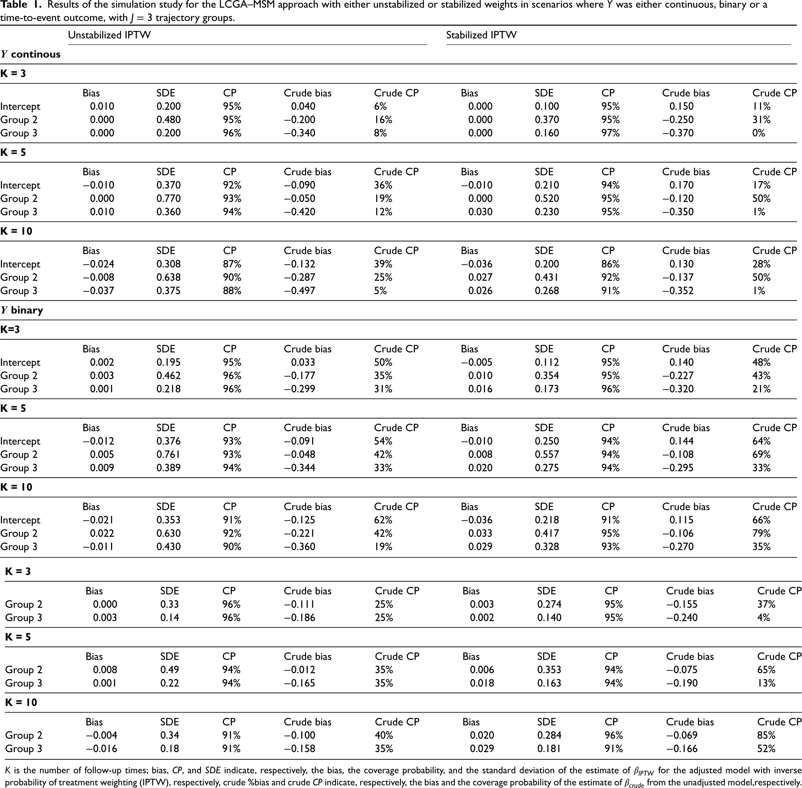
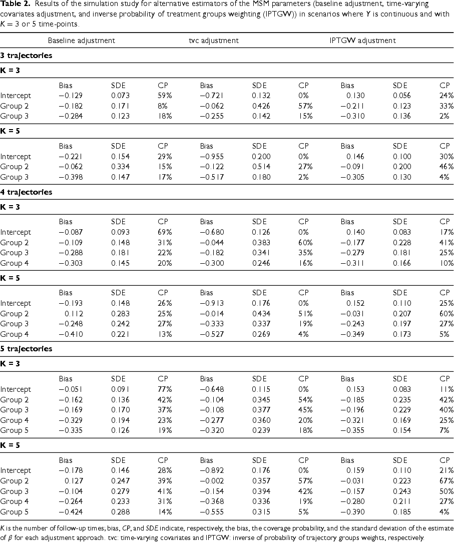
Table 1 presents the results for the LCGA–MSM and crude results for the scenarios with $J=3$ trajectory groups. Similar results were obtained in the scenarios with four or five trajectory groups (see Web Tables 1 and 2 in Supplemental Appendix C). The bias for our proposed LCGA–MSM with either unstabilized or stabilized weights was small in all considered scenarios. However, stabilized weights yielded estimates with a smaller standard deviation. The confidence intervals also tended to have better coverage when using stabilized weights in scenarios with multiple time points. Indeed, all confidence interval coverages were close to 95% (between 90% and 98%). This is likely because stabilization tended to avoid extreme outlying weight values. On the other hand, the crude model estimator had a large bias and low coverage probabilities of confidence intervals. Table 2 presents the results for alternative methods for adjusting for confounding when estimating the effect of the trajectory groups, such as adjustment for baseline covariates in the outcome model, adjustment for time-varying covariates in the outcome model and IPTGW adjusted LCGA. Recall that only scenarios where the continuous outcome case and with either $K=3$ or $K=5$ time-points were considered for these alternative methods. Regardless of the number of follow-up times and number of trajectory groups, alternative estimators of the MSM parameters were highly biased with low confidence interval coverage (between 2% and 67%), showcasing the importance of using an approach that appropriately addresses time-dependent confounding.

Table 1.

Results of the simulation study for the LCGA–MSM approach with either unstabilized or stabilized weights in scenarios where $Y$ was either continuous, binary or a time-to-event outcome, with $J=3$ trajectory groups.

	Unstabilized IPTW					Stabilized IPTW
$Y$ continous
K = 3
	Bias	SDE	CP	Crude bias	Crude CP	Bias	SDE	CP	Crude bias	Crude CP
Intercept	0.010	0.200	95%	0.040	6%	0.000	0.100	95%	0.150	11%
Group 2	0.000	0.480	95%	−0.200	16%	0.000	0.370	95%	−0.250	31%
Group 3	0.000	0.200	96%	−0.340	8%	0.000	0.160	97%	−0.370	0%
K = 5
	Bias	SDE	CP	Crude bias	Crude CP	Bias	SDE	CP	Crude bias	Crude CP
Intercept	−0.010	0.370	92%	−0.090	36%	−0.010	0.210	94%	0.170	17%
Group 2	0.000	0.770	93%	−0.050	19%	0.000	0.520	95%	−0.120	50%
Group 3	0.010	0.360	94%	−0.420	12%	0.030	0.230	95%	−0.350	1%
K = 10
	Bias	SDE	CP	Crude bias	Crude CP	Bias	SDE	CP	Crude bias	Crude CP
Intercept	−0.024	0.308	87%	−0.132	39%	−0.036	0.200	86%	0.130	28%
Group 2	−0.008	0.638	90%	−0.287	25%	0.027	0.431	92%	−0.137	50%
Group 3	−0.037	0.375	88%	−0.497	5%	0.026	0.268	91%	−0.352	1%
$Y$ binary
K=3
	Bias	SDE	CP	Crude bias	Crude CP	Bias	SDE	CP	Crude bias	Crude CP
Intercept	0.002	0.195	95%	0.033	50%	−0.005	0.112	95%	0.140	48%
Group 2	0.003	0.462	96%	−0.177	35%	0.010	0.354	95%	−0.227	43%
Group 3	0.001	0.218	96%	−0.299	31%	0.016	0.173	96%	−0.320	21%
K = 5
	Bias	SDE	CP	Crude bias	Crude CP	Bias	SDE	CP	Crude bias	Crude CP
Intercept	−0.012	0.376	93%	−0.091	54%	−0.010	0.250	94%	0.144	64%
Group 2	0.005	0.761	93%	−0.048	42%	0.008	0.557	94%	−0.108	69%
Group 3	0.009	0.389	94%	−0.344	33%	0.020	0.275	94%	−0.295	33%
K = 10
	Bias	SDE	CP	Crude bias	Crude CP	Bias	SDE	CP	Crude bias	Crude CP
Intercept	−0.021	0.353	91%	−0.125	62%	−0.036	0.218	91%	0.115	66%
Group 2	0.022	0.630	92%	−0.221	42%	0.033	0.417	95%	−0.106	79%
Group 3	−0.011	0.430	90%	−0.360	19%	0.029	0.328	93%	−0.270	35%
$Y$ time-to-event
K = 3
	Bias	SDE	CP	Crude bias	Crude CP	Bias	SDE	CP	Crude bias	Crude CP
Group 2	0.000	0.33	96%	−0.111	25%	0.003	0.274	95%	−0.155	37%
Group 3	0.003	0.14	96%	−0.186	25%	0.002	0.140	95%	−0.240	4%
K = 5
	Bias	SDE	CP	Crude bias	Crude CP	Bias	SDE	CP	Crude bias	Crude CP
Group 2	0.008	0.49	94%	−0.012	35%	0.006	0.353	94%	−0.075	65%
Group 3	0.001	0.22	94%	−0.165	35%	0.018	0.163	94%	−0.190	13%
K = 10
	Bias	SDE	CP	Crude bias	Crude CP	Bias	SDE	CP	Crude bias	Crude CP
Group 2	−0.004	0.34	91%	−0.100	40%	0.020	0.284	96%	−0.069	85%
Group 3	−0.016	0.18	91%	−0.158	35%	0.029	0.181	91%	−0.166	52%

$K$ is the number of follow-up times; bias, $CP$ , and $SDE$ indicate, respectively, the bias, the coverage probability, and the standard deviation of the estimate of ${\beta }_{IPTW}$ for the adjusted model with inverse probability of treatment weighting (IPTW), respectively, crude %bias and crude $CP$ indicate, respectively, the bias and the coverage probability of the estimate of ${\beta }_{crude}$ from the unadjusted model,respectively.

Table 2.

Results of the simulation study for alternative estimators of the MSM parameters (baseline adjustment, time-varying covariates adjustment, and inverse probability of treatment groups weighting (IPTGW)) in scenarios where $Y$ is continuous and with $K=3$ or $5$ time-points.

	Baseline adjustment			tvc adjustment			IPTGW adjustment
3 trajectories
K = 3
	Bias	SDE	CP	Bias	SDE	CP	Bias	SDE	CP
Intercept	−0.129	0.073	59%	−0.721	0.132	0%	0.130	0.056	24%
Group 2	−0.182	0.171	8%	−0.062	0.426	57%	−0.211	0.123	33%
Group 3	−0.284	0.123	18%	−0.255	0.142	15%	−0.310	0.136	2%
K = 5
	Bias	SDE	CP	Bias	SDE	CP	Bias	SDE	CP
Intercept	−0.221	0.154	29%	−0.955	0.200	0%	0.146	0.100	30%
Group 2	−0.062	0.334	15%	−0.122	0.514	27%	−0.091	0.200	46%
Group 3	−0.398	0.147	17%	−0.517	0.180	2%	−0.305	0.130	4%
4 trajectories
K = 3
	Bias	SDE	CP	Bias	SDE	CP	Bias	SDE	CP
Intercept	−0.087	0.093	69%	−0.680	0.126	0%	0.140	0.083	17%
Group 2	−0.109	0.148	31%	−0.044	0.383	60%	−0.177	0.228	41%
Group 3	−0.288	0.181	22%	−0.182	0.341	35%	−0.279	0.181	25%
Group 4	−0.303	0.145	20%	−0.300	0.246	16%	−0.311	0.166	10%
K = 5
	Bias	SDE	CP	Bias	SDE	CP	Bias	SDE	CP
Intercept	−0.193	0.148	26%	−0.913	0.176	0%	0.152	0.110	25%
Group 2	0.112	0.283	25%	−0.014	0.434	51%	−0.031	0.207	60%
Group 3	−0.248	0.242	27%	−0.333	0.337	19%	−0.243	0.197	27%
Group 4	−0.410	0.221	13%	−0.527	0.269	4%	−0.349	0.173	5%
5 trajectories
K = 3
	Bias	SDE	CP	Bias	SDE	CP	Bias	SDE	CP
Intercept	−0.051	0.091	77%	−0.648	0.115	0%	0.153	0.083	11%
Group 2	−0.162	0.136	42%	−0.104	0.345	54%	−0.185	0.235	42%
Group 3	−0.169	0.170	37%	−0.108	0.377	45%	−0.196	0.229	40%
Group 4	−0.329	0.194	23%	−0.277	0.360	20%	−0.321	0.169	25%
Group 5	−0.335	0.126	19%	−0.320	0.239	18%	−0.355	0.154	7%
K = 5
	Bias	SDE	CP	Bias	SDE	CP	Bias	SDE	CP
Intercept	−0.178	0.146	28%	−0.892	0.176	0%	0.159	0.110	21%
Group 2	0.127	0.247	39%	−0.002	0.357	57%	−0.031	0.223	67%
Group 3	−0.104	0.279	41%	−0.154	0.394	42%	−0.157	0.243	50%
Group 4	−0.264	0.233	31%	−0.368	0.336	19%	−0.280	0.211	27%
Group 5	−0.424	0.288	14%	−0.555	0.315	5%	−0.390	0.185	4%

$K$ is the number of follow-up times; bias, $CP$ , and $SDE$ indicate, respectively, the bias, the coverage probability, and the standard deviation of the estimate of $\beta$ for each adjustment approach. tvc: time-varying covariates and IPTGW: inverse of probability of trajectory groups weights, respectively.

7. Application

7.1. Data

The LCGA–MSM was applied to investigate the effectiveness of statins in primary prevention of CVD among older adults in Québec, Canada. Our aim was to estimate the effect of different statin adherence profiles on a first event of CVD. To achieve this goal, we used data from the Quebec Integrated Chronic Disease Surveillance System (QICDSS) available at the Institut National de Santé Publique du Québec (INSPQ). The QICDSS is updated annually and is composed of five linked databases ³¹ : (1) health insurance registry, (2) hospitalization database, (3) vital statistics (4) physician claims, and (5) pharmaceutical services drugs. The health insurance registry contains demographic and geographic information on all residents of the province of Quebec with a public health insurance number (99.1% in 2011–2012 of the Quebec population were eligible and admissible to the RAMQ health insurance, ³¹ ) as well as coverage by the public drug insurance plan ( $\ge$ 90% of people aged 65 and older). The hospitalization database includes data on all hospital admission, discharge dates, diagnoses, and procedures. The vital statistics database includes records on all deaths among residents of the province, including those occurring outside the province. These records are based on reports submitted by physicians or coroners, and include the date of death, the primary cause of death and other contributing causes. The physician claims database includes data on fee-for-service billings. The pharmaceutical services database contains data on drug claims including data on dates of services, name and quantity of drugs served and duration of treatment. However, information on drug claims is not available when individuals are admitted to a long-term care facility. All five databases are merged using the unique identifier of individuals that is their health insurance number. ³¹ It is noteworthy that drugs in Quebec are generally delivered for a duration of $30$ days. ³²

A retrospective cohort was extracted from the QICDSS. We identified individuals aged strictly more than $65$ years on 1 April 2013 from the province of Quebec, Canada. Because we are interested in a primary prevention context, only individuals without any CVD history in the last 5 years were included in the study. We are also interested in statin initiators (i.e. new statin users). As such, individuals with any statin claim in the year prior to enrolment were excluded. To be included, an individual was also required to be enrolled in the public drug insurance plan for at least one year prior to enrolment and throughout the study period. To minimize unmeasured confounding by indication, we only considered statin initiators and used the group of individuals with the lowest adherence as the reference group. As will be seen, this group ceased statin usage within a few months and can thus be expected to act as a good proxy for a true non-user group. We included in the cohort all statin initiators during the first 48 months of the follow-up period for a total of 52,790 statin initiators and 633,480 person-months. Each participant was followed 12 months after statin initiation (index date) to assess adherence. The outcome is a composite endpoint including non-fatal coronary heart disease, cerebral cardiovascular disease (stroke) and all-cause mortality. At the end of the exposure follow-up, events were monitored until the first of the following: death, admission to a long-term care residence or end of the administrative follow-up period on 31 March 2018. Analyses were adjusted for all available potential confounders identified through experts’ knowledge. In addition to the baseline variables sex, age, area of residence, ³³ material and social deprivation index, we also adjusted for the following time-varying covariates which were updated yearly: diabetes, hypertension, chronic kidney disease, comorbidity index, number of hospitalisations (cumulative number per year), number of visits to a specialist practitioner, number of visits to a general practitioner, number of visits to an emergency room and number of medications during the follow-up period of the exposure. The time-varying covariates are measured on an annual basis and could remain constant for most of the subjects as we followed the exposure up to one year. All these variables had no missing values except for the material and social deprivation index where the unknown values of 7.74% were treated as a category.

7.2. Analysis

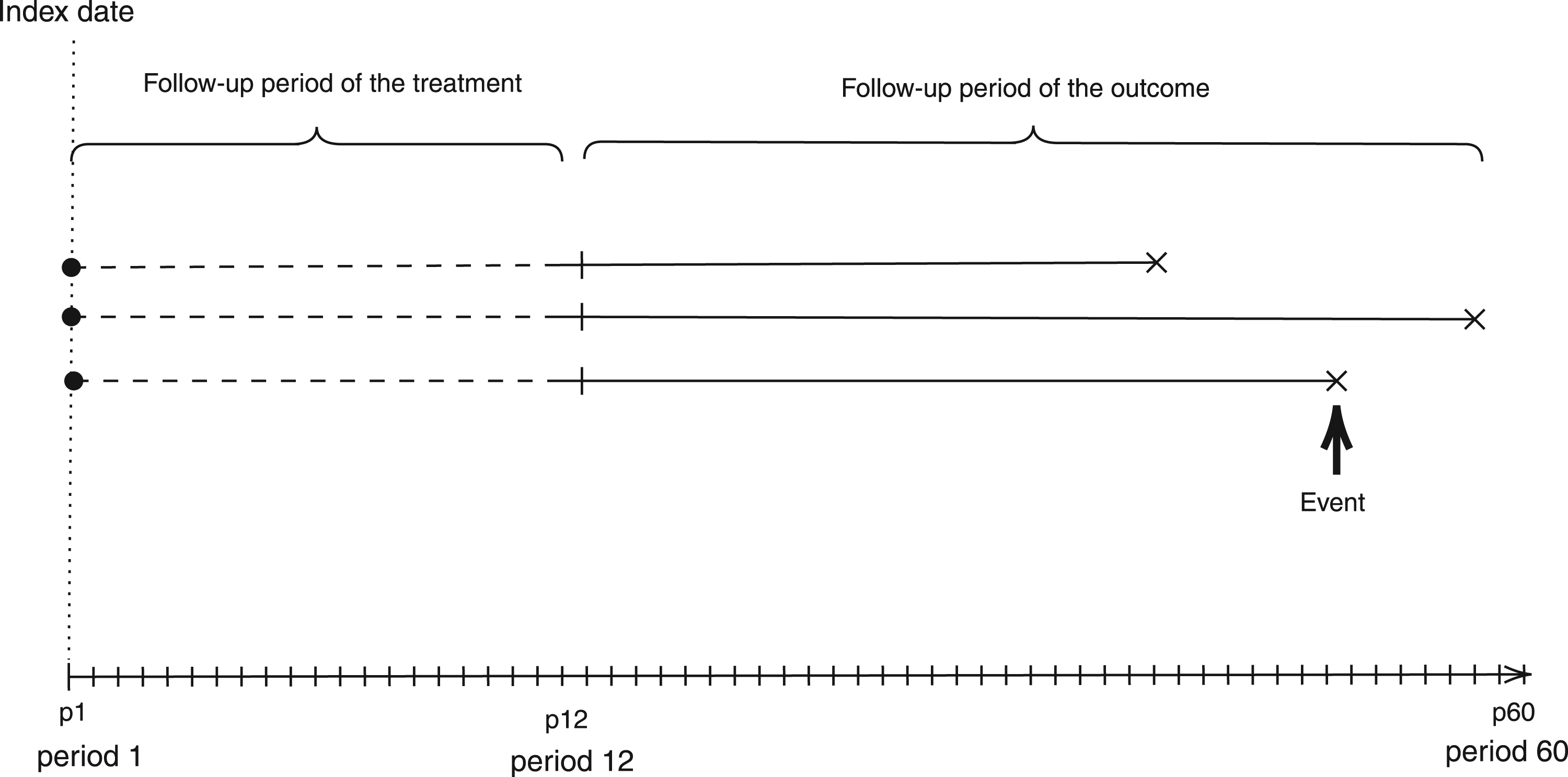
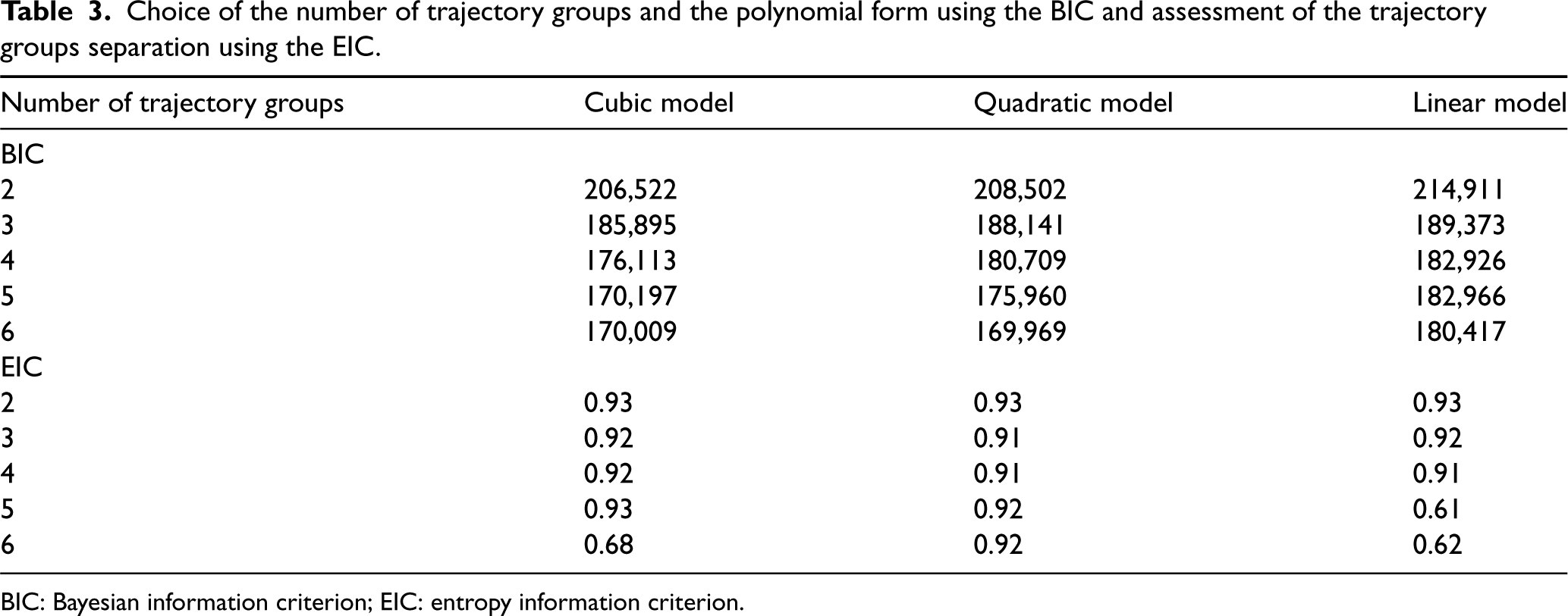
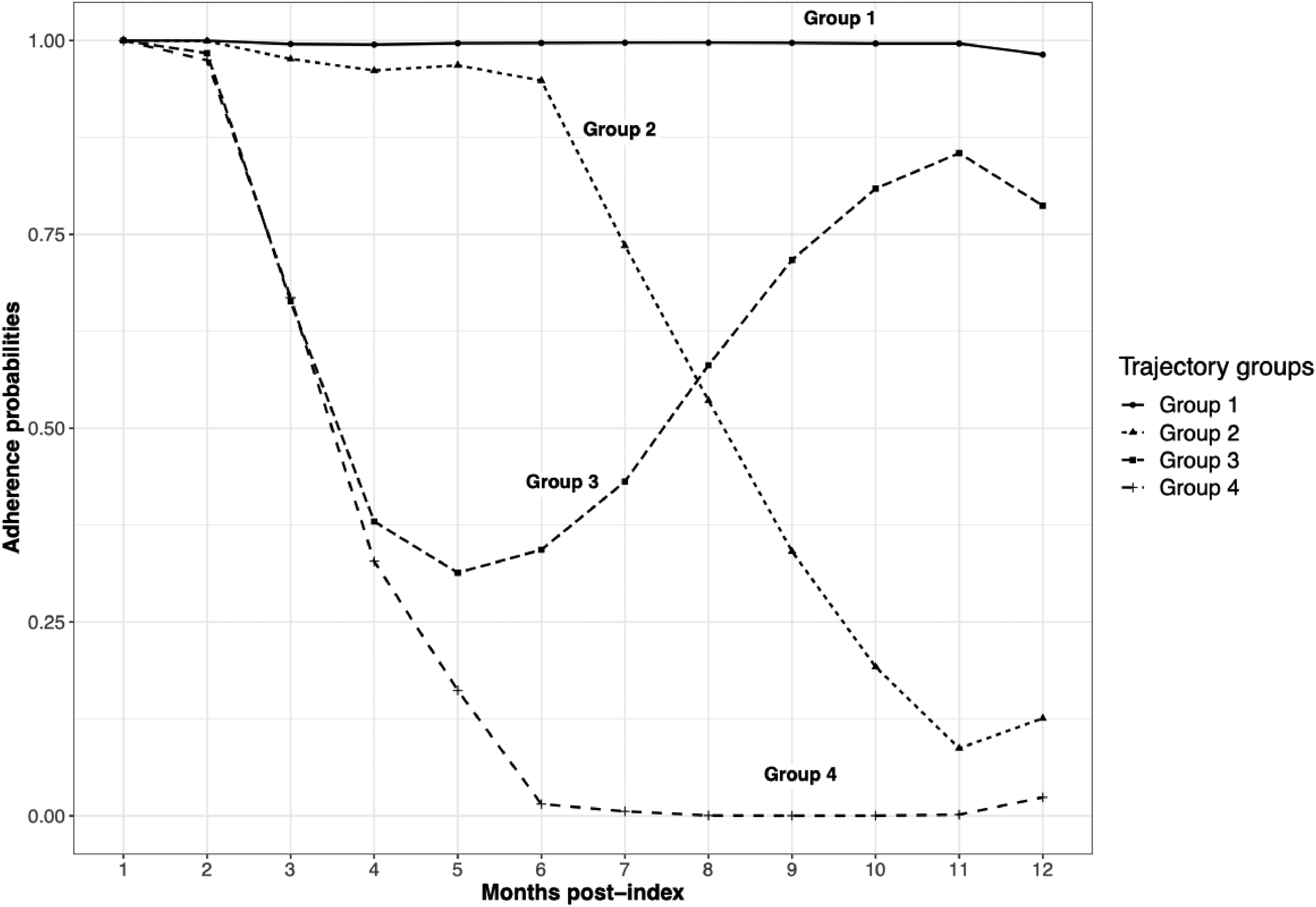
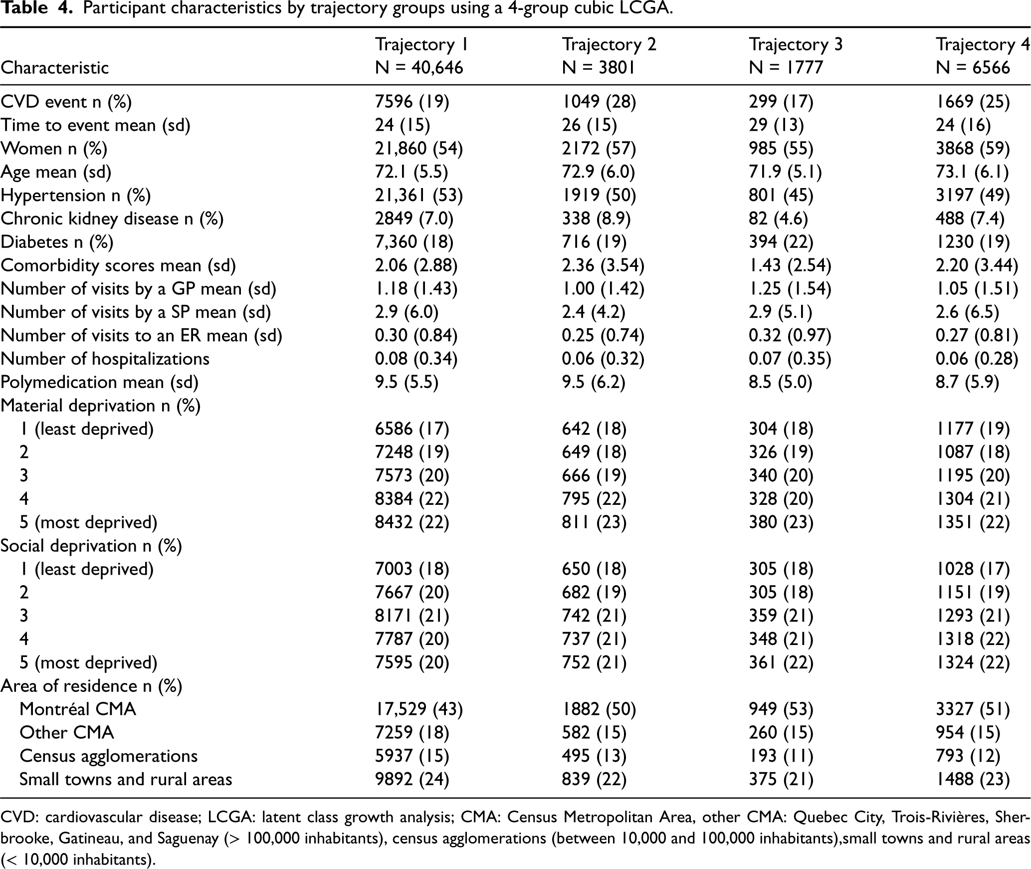
In a first step, we used LCGA to summarize $346$ unique individual treatment trajectories into a few groups. We chose the best fitting model among a set of $15$ candidate LCGA models (see Table 3). Each LCGA model is a combination of a polynomial order to model the treatment trajectories and a chosen number of trajectory groups. Individuals were assigned to a trajectory group based on their highest conditional probability to belong to that group. The best LCGA model was chosen using the BIC and the EIC. According to these criteria, the model with $6$ trajectory groups and a quadratic polynomial form was the best (BIC = 169,969 and EIC = 0.92). However, based on experts’ knowledge and to facilitate interpretation, a solution with $4$ trajectory groups was preferred (for the results with six groups, see Supplemental Appendix F). We chose to summarize the treatment trajectories with $4$ trajectory groups and a cubic model as the $EIC=0.92$ was slightly better than the $EIC=0.91$ for the quadratic model (see Figure 4). The first group was the group with the best statin adherence and comprised $77\mathrm{\%}$ (40,646) of the 52,790 statin initiators. The second included $7\mathrm{\%}$ (3801) of the individuals and was characterized by a high level of adherence throughout the first six months after initiation, followed by steep decline afterward. The trajectory in the third group featured a sharp decline in adherence between months 2 and 5, followed by an increase in adherence over the remaining months of exposure followup. This group included $3\mathrm{\%}$ (1777) of the individuals. The last group had the worst statin adherence and comprised $12\mathrm{\%}$ (6566) of participants. Trajectory groups 2 and 4 had the highest cumulative incidence of events, respectively, 28% and 25%, compared to 19% for trajectory 1 (see Table 4). Most participants were women, with more than 54% in each trajectory group. The mean age, around 72 years, was similar for all trajectory groups. The mean comorbidity score was higher in trajectory groups 2 and 4, with, respectively, 2.36 and 2.20, compared to 2.06 in trajectory 1.

Table 3.

Choice of the number of trajectory groups and the polynomial form using the BIC and assessment of the trajectory groups separation using the EIC.

Number of trajectory groups	Cubic model	Quadratic model	Linear model
BIC
2	206,522	208,502	214,911
3	185,895	188,141	189,373
4	176,113	180,709	182,926
5	170,197	175,960	182,966
6	170,009	169,969	180,417
EIC
2	0.93	0.93	0.93
3	0.92	0.91	0.92
4	0.92	0.91	0.91
5	0.93	0.92	0.61
6	0.68	0.92	0.62

BIC: Bayesian information criterion; EIC: entropy information criterion.

Figure 4.

Latent class growth analysis (LCGA) with four trajectory groups and a cubic model.

Table 4.

Participant characteristics by trajectory groups using a 4-group cubic LCGA.

	Trajectory 1	Trajectory 2	Trajectory 3	Trajectory 4
Characteristic	N = 40,646	N = 3801	N = 1777	N = 6566
CVD event n (%)	7596 (19)	1049 (28)	299 (17)	1669 (25)
Time to event mean (sd)	24 (15)	26 (15)	29 (13)	24 (16)
Women n (%)	21,860 (54)	2172 (57)	985 (55)	3868 (59)
Age mean (sd)	72.1 (5.5)	72.9 (6.0)	71.9 (5.1)	73.1 (6.1)
Hypertension n (%)	21,361 (53)	1919 (50)	801 (45)	3197 (49)
Chronic kidney disease n (%)	2849 (7.0)	338 (8.9)	82 (4.6)	488 (7.4)
Diabetes n (%)	7,360 (18)	716 (19)	394 (22)	1230 (19)
Comorbidity scores mean (sd)	2.06 (2.88)	2.36 (3.54)	1.43 (2.54)	2.20 (3.44)
Number of visits by a GP mean (sd)	1.18 (1.43)	1.00 (1.42)	1.25 (1.54)	1.05 (1.51)
Number of visits by a SP mean (sd)	2.9 (6.0)	2.4 (4.2)	2.9 (5.1)	2.6 (6.5)
Number of visits to an ER mean (sd)	0.30 (0.84)	0.25 (0.74)	0.32 (0.97)	0.27 (0.81)
Number of hospitalizations	0.08 (0.34)	0.06 (0.32)	0.07 (0.35)	0.06 (0.28)
Polymedication mean (sd)	9.5 (5.5)	9.5 (6.2)	8.5 (5.0)	8.7 (5.9)
Material deprivation n (%)
1 (least deprived)	6586 (17)	642 (18)	304 (18)	1177 (19)
2	7248 (19)	649 (18)	326 (19)	1087 (18)
3	7573 (20)	666 (19)	340 (20)	1195 (20)
4	8384 (22)	795 (22)	328 (20)	1304 (21)
5 (most deprived)	8432 (22)	811 (23)	380 (23)	1351 (22)
Social deprivation n (%)
1 (least deprived)	7003 (18)	650 (18)	305 (18)	1028 (17)
2	7667 (20)	682 (19)	305 (18)	1151 (19)
3	8171 (21)	742 (21)	359 (21)	1293 (21)
4	7787 (20)	737 (21)	348 (21)	1318 (22)
5 (most deprived)	7595 (20)	752 (21)	361 (22)	1324 (22)
Area of residence n (%)
Montréal CMA	17,529 (43)	1882 (50)	949 (53)	3327 (51)
Other CMA	7259 (18)	582 (15)	260 (15)	954 (15)
Census agglomerations	5937 (15)	495 (13)	193 (11)	793 (12)
Small towns and rural areas	9892 (24)	839 (22)	375 (21)	1488 (23)

CVD: cardiovascular disease; LCGA: latent class growth analysis; CMA: Census Metropolitan Area, other CMA: Quebec City, Trois-Rivières, Sherbrooke, Gatineau, and Saguenay (> 100,000 inhabitants), census agglomerations (between 10,000 and 100,000 inhabitants),small towns and rural areas (< 10,000 inhabitants).

In a second step, we related the outcome to the trajectory groups using a marginal structural Cox model. Note that, by construction, all participants were users at the first period. Because very few participants were non-users in periods 1 (0%), 2 (0.4%), and 3 (6%), covariate balance between treatment groups was only assessed after period 4 (see Supplemental Appendix D). Even before adjusting with IPW, there was no important difference between statin users and non-users at each period of follow-up. Before weighting, the highest standardized mean difference was around 0.16, for the age variable (see Supplemental Appendix E). This result supports that by design, our analysis has limited confounding by indication. To correct for the potential selection bias due to the censoring of participants with a CVD event, hospitalized, or admitted to a long-term care residence during the treatment follow-up period, the IPTW were multiplied by the IPCW see Cole and Hernán. ²⁸ Because of empirical positivity problems, the weights were particularly unstable after the seventh follow-up period. Hence, we performed weight truncation after considering different thresholds of truncation (99th, 99.5th, 97.5th, and 95th percentiles). ³⁴ The best covariate balance was achieved when truncating the weights at the 95th percentile, but balance did not improve as compared to the unweighted data.

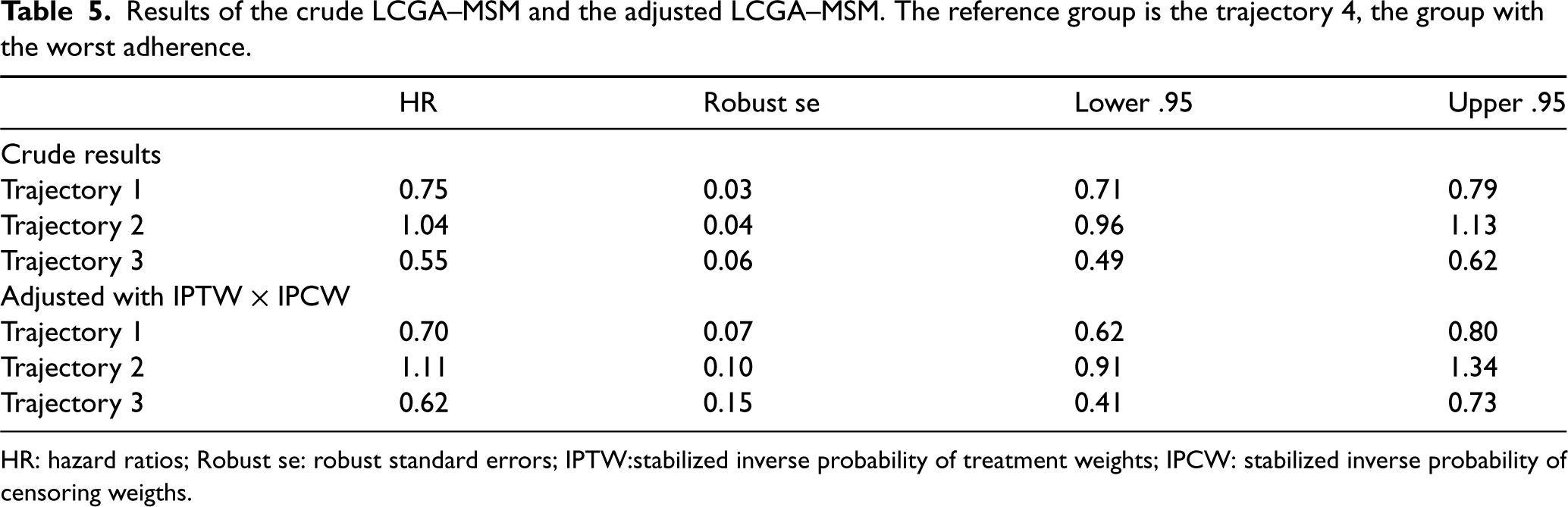
The results of the LCGA–MSM analysis are presented in Table 5. The results indicate a decreased hazard of CVD events in the group with the highest adherence versus the group with the lowest adherence ( $HR=0.70;95\mathrm{\%}IC=[0.62;0.80]$ ). Similarly, the third group, characterized by a drop in statin adherence in the second month followed by an increasing statin adherence in the fifth month, was also associated with a decreased hazard of CVD events as compared to the trajectory group with the lowest adherence ( $HR=0.62;95\mathrm{\%}IC=[0.41;0.73$ ]. The second group, represented by participants whose adherence declined after the sixth month, had slightly greater hazard of CVD events than the lowest adherence group, but the data were compatible with associations ranging from slightly protective to moderately deleterious ( $HR=1.11;95\mathrm{\%}IC=[0.91;1.34]$ ).

Table 5.

Results of the crude LCGA–MSM and the adjusted LCGA–MSM. The reference group is the trajectory 4, the group with the worst adherence.

	HR	Robust se	Lower .95	Upper .95
Crude results
Trajectory 1	0.75	0.03	0.71	0.79
Trajectory 2	1.04	0.04	0.96	1.13
Trajectory 3	0.55	0.06	0.49	0.62
Adjusted with IPTW $\times$ IPCW
Trajectory 1	0.70	0.07	0.62	0.80
Trajectory 2	1.11	0.10	0.91	1.34
Trajectory 3	0.62	0.15	0.41	0.73

HR: hazard ratios; Robust se: robust standard errors; IPTW:stabilized inverse probability of treatment weights; IPCW: stabilized inverse probability of censoring weigths.

8. Discussion

Motivated by the goal of estimating the effect of long-term adherence to statins for primary prevention of CVD among older adults, we proposed a new approach combining LCGA and MSMs. In a first step, we proposed to use LCGA to cluster individuals into a few trajectory groups based on their treatment adherence pattern, then, in a second step, choose a working MSM that relates the outcome to these groups. The parameter of interest is nonparametrically defined as the projection of the true MSM onto the chosen working causal model. This approach had two major benefits. On the one hand, we avoid assuming that we know the functional form of the true model as in a parametric model. On the other hand, we also avoid the curse of dimensionality that is often encountered when estimating a nonparametric model with finite sample data. We showed that the data-driven estimation of the trajectory groups can be ignored. As such, parameters can be estimated using the IPTW estimator and conservative inferences can be obtained using a standard robust variance estimator. Simulation studies were used to illustrate our approach and compare it with unadjusted, baseline covariates adjusted, time-varying covariates adjusted, and inverse probability of trajectory groups weighting adjusted alternatives. Scenarios with different types of outcomes (continuous, binary or time-to-event), number of follow-up times (3, 5, 10) and number of trajectory groups (3, 4, 5) were considered. In the simulation study, we found that our proposed approach yielded estimators with little or no bias whereas alternative methods were biased and had low coverage of their confidence intervals. As far as we know, such simulation studies were never performed in the literature. We also applied our approach to a population of older adults in the province of Quebec who are new statin users.

Despite the strengths of our proposed method, some limitations need to be considered. For example, in the presence of time-varying confounding, the local independence assumption of LCGA is unlikely to hold. As we have argued, this does not invalidate our proposed approach, since LCGA can simply be seen as statistical procedure of dimensionality reduction. Moreover, as mentioned by Nagin, ⁸ the groups can be seen as points of support on the unknown distribution of the observed trajectories. In that sense, the groups are not meant to represent the true data-generating process. However, when there are true groups generating the data, violation of the LCGA assumptions can lead to the identification of spurious groups.^35–37 Moreover, while the nonparametric MSM approach we have used technically avoid the risk of misspecifying the model, the effect estimates may not be informative if the observed trajectories that are clustered in the same trajectory group have very different effects. In such a situation, the “trajectory group” effect would represent an average of very different “individual trajectory” effects. In other words, for the parameter of our LCGA-MSM approach to be informative in practice, we have to assume that similar trajectories have a similar effect—which is a sensible assumption in many applications. We recommend that users conduct sensitivity analyses with different number of groups to assess the stability of effect estimates to different clustering solutions. If similar groups are found to have very different effect estimates, this may suggest that the group effect estimates do not provide an informative summary of the individual trajectory effects. Developing residual diagnostics to more directly assess if individual trajectories have similar effects would be an interesting avenue for future research. We emphasize that it is crucial to assess the quality of the clustering using tools that have been developed for LCGA, such as average posterior probabilities, odds of correct classification or entropy. Using spaghetti plots to depict the individual trajectories for each group may also be useful to assess the relative homogeneity of the trajectories that are clustered in the same group. Using a poor clustering solution or grouping together trajectories that are too different may reduce the practical interpretability and usefulness of the model. When the outcome $Y$ is binary, caution should also be exercised regarding the number of available events per trajectory group to avoid estimation problems. Furthermore, in our application, there might be residual confounding by indication that cannot be controlled. Notably, we do not have data on possibly important variables such as family history of CVD, cholesterol level or even for some cardiovascular problems that are not captured in the administrative databases.

There are various directions in which our current work could be extended. Latent class growth modeling (LCGM) can be an interesting alternative to LCGA when the goal is to capture within-group heterogeneity more effectively. LCGM allows for the identification of more nuanced trajectory groups, providing a richer representation of the underlying adherence patterns. Unlike LCGA, LCGM allows for correlated observations within a given trajectory group, thus avoiding the local independence assumption. However, LCGM is more computationally intensive than LCGA. As such, LCGA appeared to be better suited to the needs of our application, where large data were available. When deemed necessary, researchers can compare the results obtained using LCGA versus LCGM in combination with MSM. We also note that it would be possible to use a soft clustering approach wherein the dummy variables in equation (4) are replaced by the posterior probabilities of group membership. One advantage of the soft clustering approach is that it allows capturing the uncertainty in the trajectory groups attribution. However, it is also harder to define the causal parameter of interest when considering this soft clustering approach since each possible observed trajectory is no longer assigned to a single group. When developing the LCGA-MSM approach, we had initially explored the option of using soft clustering but obtained poor results in preliminary simulation studies (not shown) and did not pursue this direction. Extending our proposed approach to appropriately allow for soft clustering may be another interesting avenue for future work. Alternative ways of dealing with incomplete treatment follow-up could also be devised. For example, it would be possible to start the follow-up for events at the same time as the follow-up for treatment and assign each individual to all (complete) trajectories with which their observed (possibly incomplete) trajectory is compatible. ³⁸ Our proposed approach could also be improved by using a doubly robust estimator of the parameters of the MSM instead of the IPTW estimator. It is clear in our simulation results that the IPTW estimator failed to completely remove the bias in scenarios with multiple time points. Indeed, the IPTW estimator heavily relies on a correct specification of the probability of treatment assignment and is sensitive to near violations of the positivity assumptions. In conclusion, we believe that our LCGA-MSM can be useful to correctly estimate the effect of trajectory groups on an outcome when conducting longitudinal studies based on administrative data.

Supplemental Material

sj-pdf-1-smm-10.1177_09622802231202384 - Supplemental material for Marginal structural models with latent class growth analysis of treatment trajectories: Statins for primary prevention among older adults

Supplemental material, sj-pdf-1-smm-10.1177_09622802231202384 for Marginal structural models with latent class growth analysis of treatment trajectories: Statins for primary prevention among older adults by Awa Diop, Caroline Sirois, Jason Robert Guertin, Mireille E Schnitzer, Bernard Candas, Benoit Cossette, Paul Poirier, James Brophy, Miceline Mésidor, Claudia Blais, Denis Hamel, Mina Tadrous, Lisa Lix and Denis Talbot in Statistical Methods in Medical Research