
Abstract
Lexis diagrams are rectangular arrays of event rates indexed by age and period. Analysis of Lexis diagrams is a cornerstone of cancer surveillance research. Typically, population-based descriptive studies analyze multiple Lexis diagrams defined by sex, tumor characteristics, race/ethnicity, geographic region, etc. Inevitably the amount of information per Lexis diminishes with increasing stratification. Several methods have been proposed to smooth observed Lexis diagrams up front to clarify salient patterns and improve summary estimates of averages, gradients, and trends. In this article, we develop a novel bivariate kernel-based smoother that incorporates two key innovations. First, for any given kernel, we calculate its singular values decomposition, and select an optimal truncation point—the number of leading singular vectors to retain—based on the bias-corrected Akaike information criterion. Second, we model-average over a panel of candidate kernels with diverse shapes and bandwidths. The truncated model averaging approach is fast, automatic, has excellent performance, and provides a variance-covariance matrix that takes model selection into account. We present an in-depth case study (invasive estrogen receptor-negative breast cancer incidence among non-Hispanic white women in the United States) and simulate operating characteristics for 20 representative cancers. The truncated model averaging approach consistently outperforms any fixed kernel. Our results support the routine use of the truncated model averaging approach in descriptive studies of cancer.
Keywords
Introduction
The Lexis diagram is a fundamental construct in epidemiology, demography, and sociology. 1 A Lexis diagram is a rectangular grid of square cells with age along one axis and calendar period along the other. Individuals from a surveilled population contribute person-years and events (births, deaths, cancers, etc.) to each cell. Analysis of Lexis diagrams can elucidate temporal patterns and provide clues about the etiology of an event. 2 Notably, the analysis of Lexis diagrams is a cornerstone of cancer surveillance research.
Population-based cancer rates usually exhibit Poisson-type variability. 3 This is the default mode for analysis, although negative binomial models are available that accommodate more flexible mean-to-variance relationships.4–6 Within any given Lexis diagram, intrinsic variability (“noise”) can mask important signals and limit the power of comparative analyses to identify heterogeneity. In epidemiologic research, the classic approaches deal with intrinsic variability by aggregating granular data (e.g. data originally sampled at the scale of a single-years of age and/or calendar years) into broader age and period categories, 7 typically, 5-year age groups. Unfortunately, there is nothing optimal about such traditional groupings.
Several methods have been proposed to de-noise or smooth an observed Lexis diagram before the usual descriptive7–9 and analytical 10 methods are applied. Keiding 1 pioneered the first such approach using bivariate kernel functions. This was a major advance; however, this classic method has two major limitations. First, the choice of kernel is arbitrary, hence so too is the implicit bias-variance trade-off. Second, the estimated variance-covariance matrix does not reflect uncertainty arising from kernel (model) selection. In practice, analysts tend to use small bandwidths to minimize bias rather than variance. However, there is no evidence that such choices are optimal.
Other investigators have developed more sophisticated methods. Currie et al. 11 produced smooth Lexis diagrams using bivariate P-splines and second-difference penalty functions. Camarda 12 implemented the Currie approach in R and developed methods to incorporate established demographic constraints using asymmetric penalties. 13 Dokumentov et al. 14 developed a hybrid approach that combines smoothing methods with additional parameters that account for abrupt changes in age incidence by period and cohort. Chien et al.15,16 developed a fully Bayesian smoothing approach using two-dimensional Bernstein polynomials, data-dependent prior distributions, and the Metropolis-Hastings reversible jump algorithm. Martinez-Hernandez and Genton 17 developed nonparametric methods for the situation where the data can be viewed as a functional trend in one temporal dimension (e.g. age) that is modulated over the other dimension (e.g. time).
In this article, we develop a novel and complementary kernel-based approach using truncated bivariate kernel functions18–20 and information theory. 21 We refer to these algorithms as “filters” and the outputs as “filtrations” because they do more than simply “smooth” the data: by design, they pass through all signals that materially reduce the within-Lexis mean squared error. Our approach has several attractive features. It is fast, and automatic, provides the smoothest possible kernel-based estimates consistent with data, yields a variance–covariance matrix that takes model selection into account, and has excellent performance.
In Section 2, we review notation and background on Lexis diagrams and kernel functions and assemble a representative panel of incident cancers. In Section 3, we describe the new filters and corresponding variance calculations. In Section 4, we illustrate our proposed methods using invasive estrogen receptor (ER)-negative breast cancer incidence among non-Hispanic white women in the United States, and in Section 6, we simulate our method's operating characteristics over the cancer incidence panel. In Section 7, we give a summary and discuss avenues for future research. We provide technical details in an online supplement. Our R code is freely available upon request.
Background
Event rates on a Lexis diagram
We begin with a brief overview of the Lexis diagram and introduce our notation.
22
A Lexis diagram is a rectangular field with attained age a along the y-axis and calendar time p along the x-axis. For any given population and outcome, individual event times and corresponding person-years at risk are summed beginning at age


Cancer incidence panel
We extracted authoritative cancer incidence data for the United States from the Surveillance, Epidemiology, and End Results Program's Thirteen Registries Database (SEER-13 23 ) for 50 single-years of age (ages 35–84) and 27 calendar years (1992–2018). We selected a panel of representative scenarios defined by cancer site (14 cancers associated with obesity 24 ), sex, and standard SEER race/ethnicity categories (Table 1 and Supplemental Part A). We redistributed breast cancer cases with missing or unknown ER status to the corresponding age- and year-specific ER positive and negative cells using a validated approach.25,26 The panel includes a total of 1,049,633 incident cases.
Kernel functions
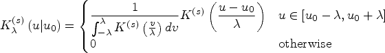
See Supplemental Part B for details. The standard form of a univariate kernel function
20
is represented by a canonical “shape” function
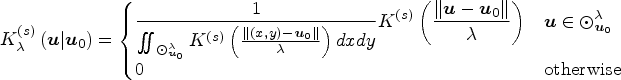
We can extend a univariate kernel for use in two isotropic spatial dimensions by expressing its formula as a function of the Euclidean distance between any given point
Kernel function analysis
Kernel filtration
Our kernel function analysis is motivated by the classic domain filtering approach of image processing 27 which itself is motivated by classic kernel methods in statistics.20,28,29 For images, bivariate kernels are used to construct mean or low-pass “blurring” filters for purposes of “de-noising” the observed pixel values and/or reducing the impact of high-frequency signals.30,31 We apply bivariate kernels to Lexis diagrams for the same purposes. A standard kernel function analysis 29 is described in Algorithm 1.
Choose a kernel shape box, trg, Epan, or triwt. Choose a bandwidth Repeat steps 3–6 for each cell. Superimpose a masking circle of radius Calculate kernel weights for all cells whose mid-points are covered by the masking circle. Divide each weight in step 4 by their sum (normalization). Use the normalized weights to calculate a weighted average of the corresponding
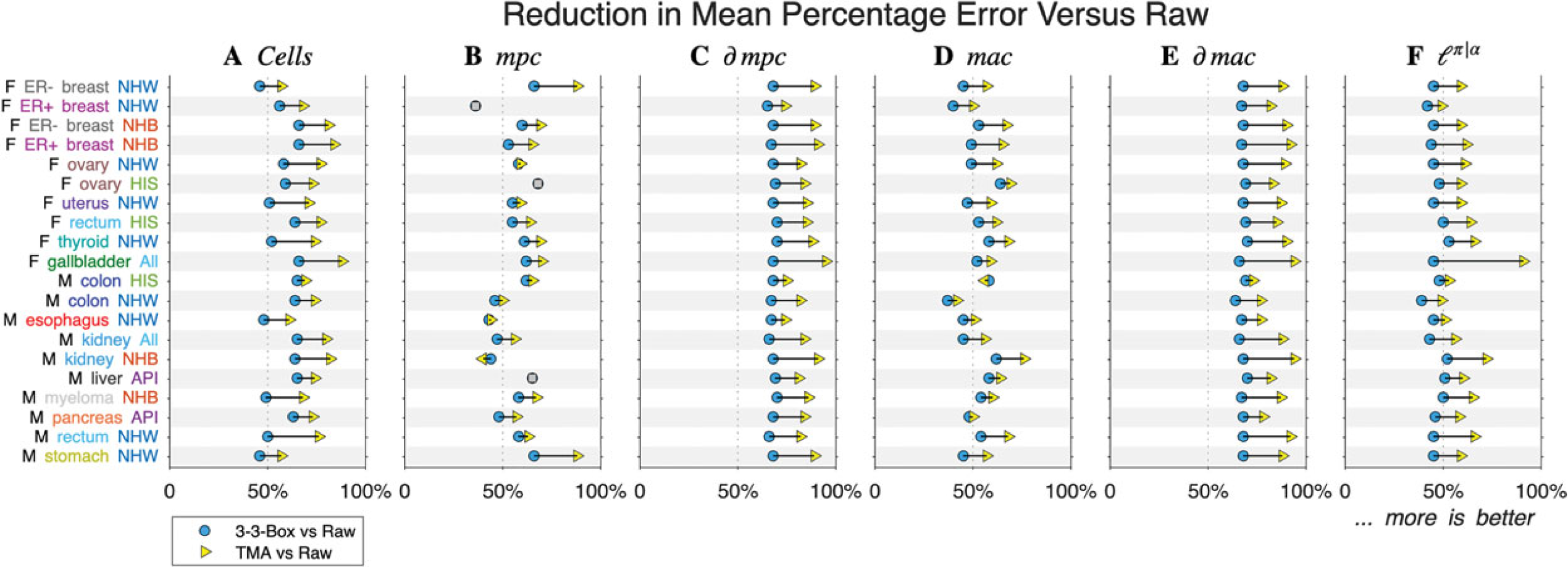
We will refer to the vector of weighted averages as
Cancer panel.
a
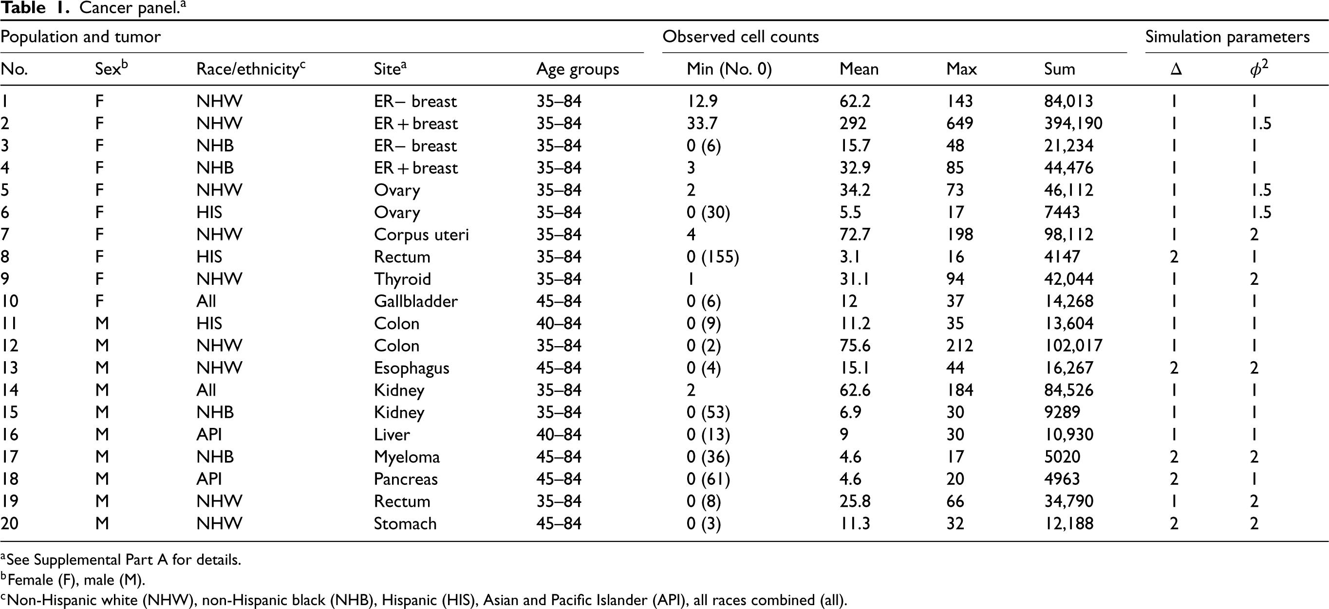
Cancer panel. a
See Supplemental Part A for details.
Female (F), male (M).
Non-Hispanic white (NHW), non-Hispanic black (NHB), Hispanic (HIS), Asian and Pacific Islander (API), all races combined (all).
The evaluation grid is discrete, while the possible bandwidths
Surprisingly, the bivariate kernels used in Algorithm 1 are invertible or nearly so. It follows that little or no information is discarded by these kernels. Their application allows “smooth” signals to pass through almost unchanged, while at the same time, complex variable signals are downweighted. Although the kernel operators are sparse, their inverses are dense.
We these results in hand we can present our “rule-of-thumb” over-dispersion estimator

We hypothesized that we could regularize the output of a filter
Choose a kernel Construct the SVD of Consider the sequence of truncated kernels For each value of
Center the data using the inverse-variance weighted average,
Consider s to be the effective degrees of freedom or
Calculate the residual vector
Calculate the bias-corrected Akaike information criterion statistic
The best-fit model uses The fitted values are 
Use of the bias-corrected penalty term is essential to avoid over-fitting, 21 especially for “small” Lexis diagrams with a relatively small total number of cells. The bias-corrected AIC serves as a compromise between the classic uncorrected AIC, which overfits when the number of unknown terms is large relative to the amount of data, and the classic BIC, which is known to be overly conservative producing poorly fitting results. 21
We now have three versions of the data: the observed or “raw” data
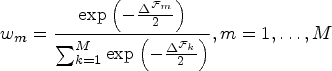
Select a panel of Apply Identify the optimal kernel For each kernel identified in step 3, identify all cut-off values c whose Calculate Akaike weights
Calculate the truncated model average filtration
Calculate the unconditional (model-averaged) variance-covariance matrix

There is no penalty other than computation time for using a comprehensive panel of kernels. We used 48 kernels in our case study and simulations (Supplemental Part B).
Variance calculations
Each algorithm produces a variance-covariance matrix that allows us to set confidence limits for any given cell, or for any set of linear combinations of cells. Let
Given C linear combinations of
To analyze log-transformed rates
Results
Case study: Invasive ER− breast cancer incidence among non-Hispanic white women
Invasive female breast cancer is the most common malignancy among women, and its epidemiology varies by tumor subtype. 33 Two major subtypes are ER-positive (ER+) and ER-negative (ER−) tumors. 33 For reasons that remain unclear, the incidence of ER− breast cancer has been decreasing over time in many populations around the world, and the rate of decrease over time varies by age.5,34–37 In this case study, we apply our new methods to SEER data on invasive ER− breast cancer incidence among non-Hispanic white women (Table 1, No. 1).
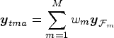
Figure 1(A) presents a heat map of the observed rates per 100,000 women years. There is considerable variability from cell to cell, but the data are not over-dispersed (
Estrogen receptor-negative breast cancer incidence among non-Hispanic white women. Raw data (panels A–C), benchmark kernel (panels D – F), and truncated model average (panels G – I). Left panels: Lexis diagram heat maps. Center panels: Rates over time within 5-year age groups. Right panels: Rates by age within 5-year calendar periods. Shaded envelopes show 95% point-wise confidence limits.
Figure 1(D) to (F) repeats these analyses using outputs from the benchmark all-in kernel. Panel 1D presents a heat map based on
Figure 1(G) to (I) repeats these analyses using the filtered data
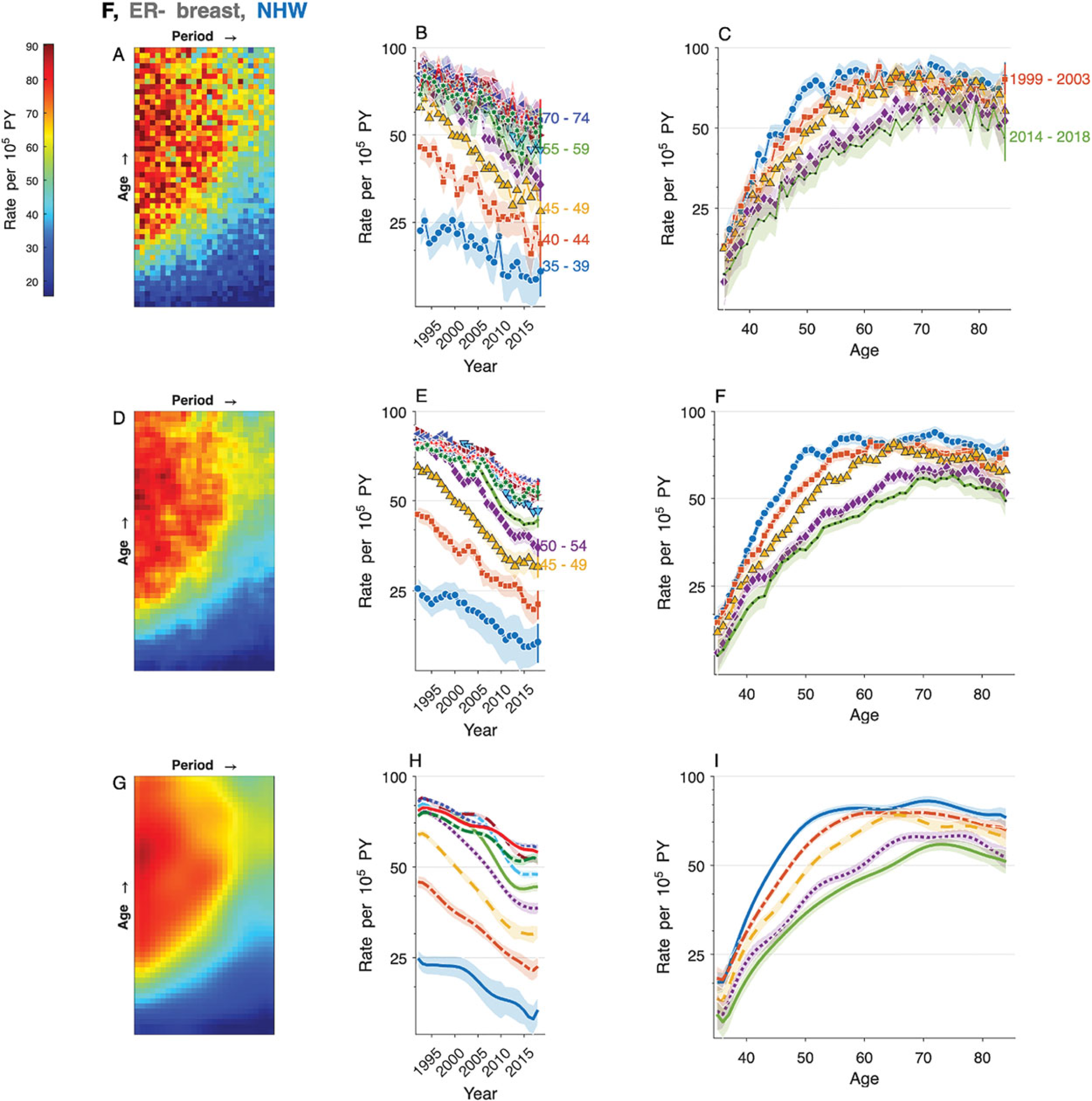
Graphs provide insight, but no descriptive study is complete until salient features that may be apparent in graphs are quantified using objective and reproducible statistics. There is latitude regarding the precise feature set8,10; widely used features obtain from averages, gradients, and trends. We consider five features that together quantify the marginal effects of period and age as well as interactions between period and age.
The marginal period curve The marginal age curve The slope of the age-specific log rates over time,
Each feature is a linear function of the log rates; therefore, each can be extracted using a corresponding contrast matrix
Figure 2(A) to (C) presents these features calculated from the observed data
Breast cancer averages, gradients, and trends. Features extracted from the data are shown in Figure 1. Raw data (panels A–C), benchmark kernel (panels D – F), and truncated model average (panels G – I). Left panels: Marginal period curve (left axis) and gradient (right axis). Center panels: Marginal age curve (left axis) and gradient (right axis). Right panels: Age-specific period trends. Gradient estimates in the left and center panels are trimmed to exclude the first and last time points. Shaded envelopes show pointwise 95% confidence limits.
The marginal age curve (
The incidence decreases over time in every age group at a rate that varies by age (
We assessed the operating characteristics of our algorithms by simulating the 20 cancers in Table 1. See Supplemental Part F for details. In five scenarios, we blocked the data into
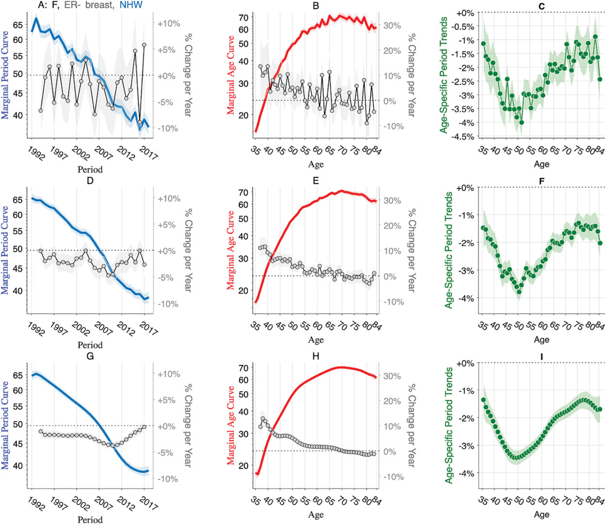
In every scenario, TMA produced more accurate heat maps than the benchmark kernel (Figure 3(A)). Compared to analyzing the raw data, the benchmark kernel reduced the mean percentage error by 58% on average over the 20 scenarios, versus 74% for TMA.
Arrow plots of simulation results. Rows correspond to 20 cancers summarized in Table 1. Panels correspond to features. Blue circles show a percent reduction for benchmark kernel versus raw, and yellow triangles show a percent reduction for truncated model average (TMA) versus raw.
Performance gains for
How did TMA achieve such gains in performance? The rule-of-thumb over-dispersion estimator, estimated in step 2 and used in step 4 of Algorithm 2, appears adequate (Figure 4(A)). On average over the 20 scenarios, the median value of
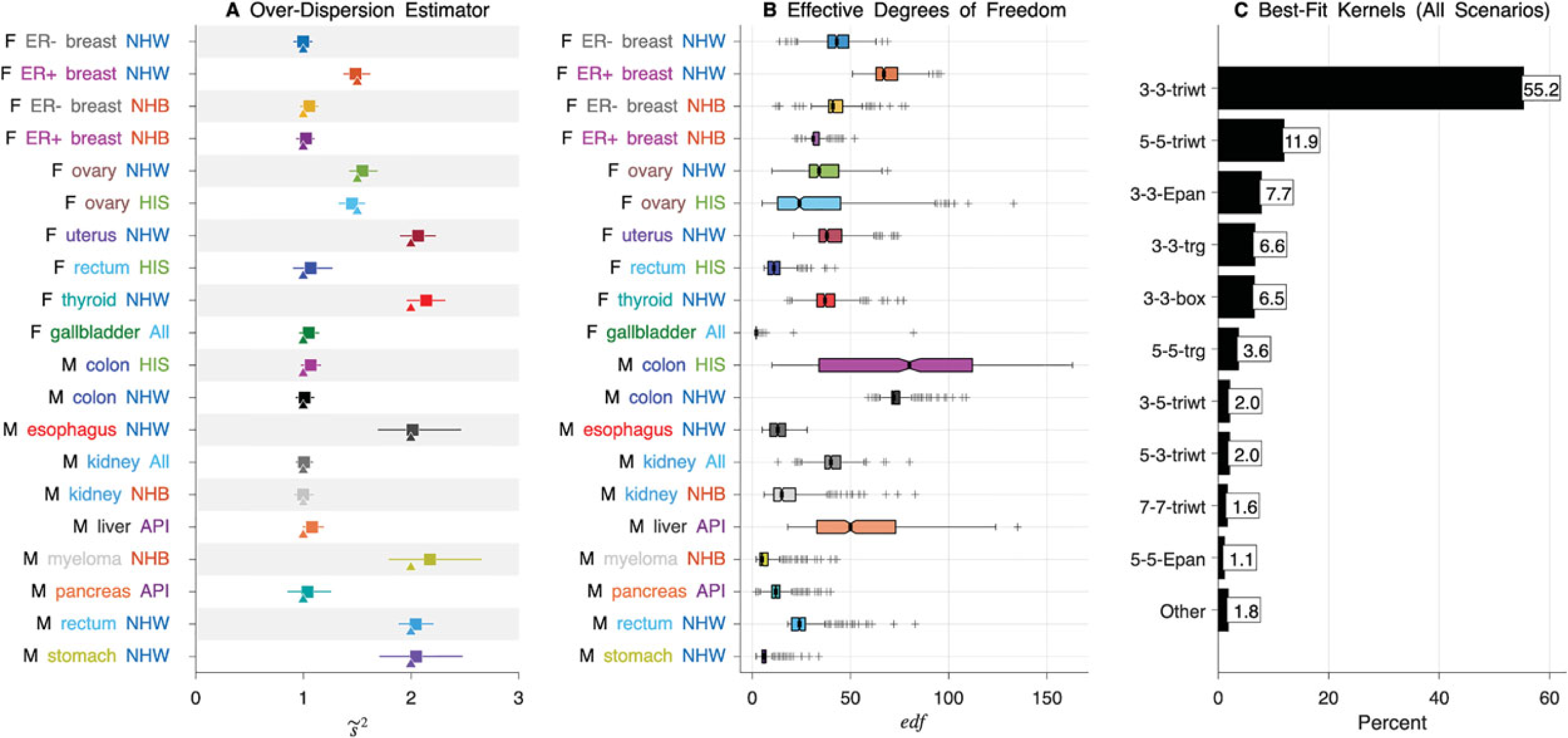
Operating characteristics of truncated model average. (A) Rows correspond to 20 cancers summarized in Table 1. Median (squares) and 90% limits (bars) of the estimated over-dispersion parameter (
In all scenarios,
We developed a novel non-parametric approach to regularize (“smooth”) event rates ascertained over Lexis diagrams. Our methods borrow smoothing concepts from time series analysis, that is, k-point moving averages, and classic multivariate kernel methods in statistics 29 and image processing, that is, filtering and singular values decomposition. Our approach uses statistical information theory, specifically, the bias-corrected AIC, 21 to handle the model selection problem and provide a variance–covariance matrix that takes model selection into account.
Our truncated model averaging approach adds to the armamentarium and complements existing non-parametric12,13,17 and Bayesian 15 methods. The kernel-based methods developed by Duong and Hazelton 29 are closest in spirit to our approach. In our approach, we use bias-corrected AIC versus cross-validation, and we use truncated kernels versus full kernels, which, as we show, substantially increases accuracy.
Our approach to selecting effective degrees of freedom to quantify the complexity of the underlying Lexis diagram is similar to approaches used to select basis functions in generalized additive models. 38 Furthermore, Gaussian process-based smoothing can be viewed as special case of our new bivariate methods since the Matérn covariance used in previous work 39 encompasses both the Exponential and Gaussian kernels, both of which are similar to the triweight kernel. Interestingly, in our simulations, the triweight kernel was by far the most frequently selected kernel shape.
Examination of smoothed Lexis diagrams provides a good overview. Subsequently, scientific conclusions obtain from quantifications of averages, gradients, and trends. As illustrated by our case study, not only does the truncated model averaging approach provide appealingly smoothed heat maps (Figure 1), but corresponding linear combinations of the smoothed values are also substantially more precise (Figure 2).
As shown by our simulation studies, when the cells of the observed Lexis diagrams are statistically independent quasi-Poisson variates, Algorithm 3 (truncated model averaging) is superior to any fixed kernel. Indeed, compared to our benchmark kernel, the truncated model average reduced the intrinsic root mean squared error by 60%–86% depending on the feature.
We focused here on Lexis diagrams, but our methods and software can be applied when the data follow an approximate multivariate normal distribution with a full-rank covariance matrix known up to a scale parameter. Sparse cell counts are an issue in the Poisson case. We implemented our methods using the Normal approximation to the Poisson distribution, which worked well in all scenarios considered (Table 1). If single-year data are sparse (numerous zeros) one can increase the bin width. Future research might consider incorporating a standard or zero-inflated Poisson log-likelihood function. More advanced kernels could also be investigated, for example, steering kernels. 27 Indeed, our model averaging approach could be extended to include estimates obtained using complementary methods such as steering kernels or splines.
In cancer surveillance research few studies examine a single Lexis diagram in isolation. Rather, hypotheses are generated by examining related Lexis diagrams defined by sex, race/ethnicity, geographic region, tumor characteristics, etc. Invariably the amount of information per Lexis diminishes with increasing stratification. As demonstrated here, our new truncated model averaging approach can advance such descriptive studies.
In future work, truncated model averaging might be extended to incorporate as covariates the effects of sex, race/ethnicity, etc. For example, one could start with a joint parametric fit, for example, a proportional hazards age-period-cohort model, 40 then apply truncated model averaging to the residuals to characterize any lack-of-fit.
Supplemental Material
sj-docx-1-smm-10.1177_09622802231192950 - Supplemental material for Smoothing Lexis diagrams using kernel functions: A contemporary approach
Supplemental material, sj-docx-1-smm-10.1177_09622802231192950 for Smoothing Lexis diagrams using kernel functions: A contemporary approach by Philip S Rosenberg, Adalberto Miranda Filho, Julia Elrod, Aryana Arsham, Ana F Best and Pavel Chernyavskiy in Statistical Methods in Medical Research
Footnotes
Acknowledgements
This research was funded by the Intramural Research Program of the National Cancer Institute, Division of Cancer Epidemiology and Genetics. AMF is also supported through an appointment to the National Cancer Institute (NCI) ORISE Research Participation Program under DOE contract number DE-SC0014664.
Data accessibility
Our freely available R code and example data are available upon request.
Declaration of conflicting interests
The author(s) declared no potential conflicts of interest with respect to the research, authorship, and/or publication of this article.
Funding
The author(s) disclosed receipt of the following financial support for the research, authorship, and/or publication of this article: This work was supported by the ORISE Research Participation Program, Division of Cancer Epidemiology and Genetics, National Cancer Institute (grant number DOE contract DE-SC0014664, Intramural Research Program).
Supplemental material
Supplemental material for this article is available online.
References
Supplementary Material
Please find the following supplemental material available below.
For Open Access articles published under a Creative Commons License, all supplemental material carries the same license as the article it is associated with.
For non-Open Access articles published, all supplemental material carries a non-exclusive license, and permission requests for re-use of supplemental material or any part of supplemental material shall be sent directly to the copyright owner as specified in the copyright notice associated with the article.