Estimating transformations for evaluating diagnostic tests with covariate adjustment

Abstract

Receiver operating characteristic analysis is one of the most popular approaches for evaluating and comparing the accuracy of medical diagnostic tests. Although various methodologies have been developed for estimating receiver operating characteristic curves and their associated summary indices, there is no consensus on a single framework that can provide consistent statistical inference while handling the complexities associated with medical data. Such complexities might include non-normal data, covariates that influence the diagnostic potential of a test, ordinal biomarkers or censored data due to instrument detection limits. We propose a regression model for the transformed test results which exploits the invariance of receiver operating characteristic curves to monotonic transformations and accommodates these features. Simulation studies show that the estimates based on transformation models are unbiased and yield coverage at nominal levels. The methodology is applied to a cross-sectional study of metabolic syndrome where we investigate the covariate-specific performance of weight-to-height ratio as a non-invasive diagnostic test. Software implementations for all the methods described in the article are provided in the tram add-on package to the R system for statistical computing and graphics.

1. Introduction

Estimating receiver operating characteristic (ROC) curves for evaluating the performance of medical diagnostic tests has been a main focus of statistical literature over the last decades.^1,2 Diagnostic tests screen for the presence or absence of a disease. Characterizing their accuracy is essential to ensure appropriate prevention, treatment and monitoring of diseases. ROC curves are a valuable tool in determining the diagnostic potential of a test and continue to be extensively applied in biomedical studies as new tests or biomarkers are developed in radiology, oncology, genetics, and other related fields. Increasingly more applications can be expected due to advancements in technology and analyzing the resulting data requires a computationally straightforward approach to provide accurate and consistent statistical inference.

Previous research has focused on extending statistical methodology for ROC curve estimation to address issues such as adjustment for covariates,^3,4 incorporating censoring due to instrument detection limits^5,6 and robustness to model misspecification. ⁷ In addition, a wide variety of parametric and nonparametric methods have been proposed within frequentist and Bayesian paradigms (see Inácio et al. ⁸ for a recent review). However, there is no consensus on an analytic approach that can handle all these issues simultaneously.

An attractive feature of the ROC curve, which has scantly been used for its estimation, is that it remains invariant to monotonic transformations of the test results. Although transformations have been used to bring continuous test results into a form that approximately satisfies the assumptions of a suitable parametric model, ⁴ estimation of a transformation function has been limited to the Box-Cox power transformation family.^9,10 For rank-based methods, the transformation function can be left unspecified, but in all cases, a restriction to normality has been previously imposed on the model for the ROC curve. ¹¹

In this article, we present a new unifying methodological framework for estimating ROC curves and its associated summary indices by modeling the relationship between the transformed test results and potential covariates. We employ transformation models to jointly estimate the transformation function and regression parameters.^12,13 This approach specifies a parametric model for the ROC curve but remains distribution-free because we do not impose any strong assumptions about the transformation function. Using the estimated parameters, we show how to evaluate covariate effects on the discriminatory performance of diagnostic tests. Unlike nonparametric methods which are flexible but difficult to interpret and implement, transformation models excel on both fronts. R implementations of all methods discussed in this article are available, along with a set of supporting examples.

1.1. Notation and preliminaries

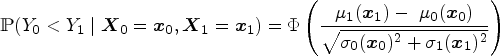
Let the random variable $Y$ denote the continuous result of a diagnostic test and let $D$ denote the disease status, with $D=1$ if a subject is diseased and 0 if nondiseased. We denote quantities conditional on the disease status using subscripts. For example, $Y_1$ and $Y_0$ are the test results in the diseased and nondiseased populations with cumulative distribution functions (CDFs) given by $F_1$ and $F_0$ and densities $f_1$ and $f_0$ , respectively. Suppose that the subject is diagnosed as diseased when their test result exceeds a threshold value, $c$ . By convention, we assume that larger values of the test result are more indicative of the disease. The probability of truly identifying a diseased and nondiseased subject is defined as sensitivity, $\mathbb{P}(Y_1>c)=1-F_1(c)$ , and specificity, $\mathbb{P}(Y_0\le c)=F_0(c)$ , respectively. The set of pairs $(1-\text{specificity},\text{sensitivity})$ for all $c\in \mathbb{R}$ produce the ROC curve. By setting $p=1-F_0(c)$ , an equivalent representation of the ROC curve is

$$\text{ROC}(p)=1-F_1(F_0^{-1}(1-p))$$

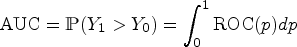
Summary indices of the ROC curve quantify the degree of separation between the distributions $Y_1$ and $Y_0$ . The most widely used index is the area under the ROC curve (AUC) defined by

$$\text{AUC}=\mathbb{P}(Y_1>Y_0)={\int }_0^1\text{ROC}(p)dp$$

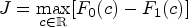
The AUC represents the probability that the test results of a randomly selected diseased subject exceed the one of a nondiseased subject and is directly related to the Mann–Whitney–Wilcoxon U-statistic (MWW). ¹⁴ Alternative indices include the Youden index, ¹⁵ $J$ , which combines sensitivity and specificity over all possible thresholds to provide the maximum potential effectiveness of a diagnostic test, given by

$$J=\underset{c\in \mathbb{R}}{max}[F_0(c)-F_1(c)]$$

The Youden index is equivalent to the Smirnov (or the two-sample Kolmogorov-Smirnov) test statistic ¹⁶ and can be represented as half the $L_1$ distance between the two densities or as the complement of the overlapping coefficient (OVL)^17–20:

$$J=\frac{1}{2}\int |f_0(y)-f_1(y)|dy=1-\int min[f_1(y),f_0(y)]dy=1-\text{OVL}$$

Additionally, the threshold corresponding to $J$ , where sensitivity and specificity are maximized, denoted as $c^{*}$ , is often used in clinical practice as the optimal classification threshold to screen subjects.

Covariates may impact the level and the accuracy of a diagnostic test. In order to appropriately understand the accuracy of the test in subpopulations, we can use covariate-specific or conditional ROC curves. ²¹ Let $\mathit{X}$ denote a vector of covariates that are hypothesized to have an impact on the accuracy of the test. The conditional CDF in the diseased population is given by $F_1(y\mid \mathit{x})=\mathbb{P}(Y_1\le y\mid \mathit{X}=\mathit{x})$ and analogously given for the nondiseased population. The covariate-specific ROC can be written as

$$\text{ROC}(p\mid \mathit{x})=1-F_1(F_0^{-1}(1-p\mid \mathit{x})\mid \mathit{x})$$

(1)

with its counterpart conditional summary indices, $\text{AUC}(\mathit{x})$ and $J(\mathit{x})$ , defined accordingly. The covariate-specific ROC curve can be generated by modeling the conditional distribution of the test results, known as the induced or indirect methodology. ³

1.2. Overview

The article proceeds as follows. In Section 2, we propose a transformation modeling framework for parameterizing ROC curves from which we derive closed-form expressions for associated AUC and Youden summary indices. We discuss maximum likelihood estimation procedures for our model and corresponding inference. In Section 3, we assess the empirical performance of our methods using simulated data. We apply our approach to a cross-sectional study for detection of metabolic syndrome in Section 4 and conclude the article with a discussion.

2. Methods

2.1. Transformation model

The ROC curve is a composition of distribution functions and thus is invariant to strictly monotonically increasing transformations of $Y$ . We propose a model for the conditional distribution of the transformed test result given the disease status and covariates. This transformation is obtained from the data and leads to a distribution-free framework to parameterize the covariate-specific ROC curve and its summary indices.

Suppose there exists a strictly monotonically increasing function $h$ such that the relationship between the transformed test result and the covariates follows a shift-scale model

$$h(Y)={\mu }_d(\mathit{x})+{\sigma }_d(\mathit{x})Z$$

where $D=d$ specifies the disease indicator ( $D=0$ for nondiseased and $D=1$ for diseased), $\mathit{X}=\mathit{x}$ a fixed set of covariates, ${\mu }_d(\mathit{x})$ is the shift term, ${\sigma }_d(\mathit{x})$ is the scale term, and $Z\in \mathbb{R}$ is a latent random variable with an a priori known absolutely continuous log-concave CDF, $F_Z$ . Given that $D$ and $\mathit{X}$ are fixed, the conditional CDF for $Y$ is

$$\mathbb{P}(Y\le y\mid D=d,\mathit{X}=\mathit{x})=F_d(y\mid \mathit{x})=F_Z\left(\frac{h(y)-{\mu }_d(\mathit{x})}{{\sigma }_d(\mathit{x})}\right)$$

(2)

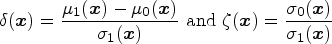
Equation (2) represents a general class of models called transformation models.^22,13 The transformation function $h$ uniquely characterizes the distribution of $Y$ , similar to the density or distribution function. Plugging in this conditional CDF of $Y$ into equation (1), $h$ cancels out and the covariate-specific ROC curve is given by

$$\text{ROC}(p\mid \mathit{x})=1-F_Z(\zeta (\mathit{x})F_Z^{-1}(1-p)-\delta (\mathit{x}))$$

(3)

where

$$\delta (\mathit{x})=\frac{{\mu }_1(\mathit{x})-{\mu }_0(\mathit{x})}{{\sigma }_1(\mathit{x})}\text{ and }\zeta (\mathit{x})=\frac{{\sigma }_0(\mathit{x})}{{\sigma }_1(\mathit{x})}$$

Thus, the ROC curve is completely determined by the shift and scale terms of the model.

The binormal ²³ and bilogistic ²⁴ ROC curves can be obtained by setting $F_Z$ to the standard normal distribution function ${\mathrm{probit}}^{-1}=\mathrm{\Phi }$ , or the standard logistic distribution function ${\mathrm{logit}}^{-1}(x)=\mathrm{expit}(x)=(1+\exp (-x){)}^{-1}$ , in equation (3), respectively. Similarly, the proportional hazard ²⁵ and reverse proportional hazard alternatives ²⁶ for the ROC curve also fall within the purview of our transformation model with $F_Z$ specified as ${\mathrm{cloglog}}^{-1}(x)=1-\exp (-\exp (x))$ (minimum extreme value distribution function) and ${\mathrm{loglog}}^{-1}(x)=\exp (-\exp (-x))$ (maximum extreme value distribution function), respectively.

However, to the best of our knowledge, the only literature where the transformation function $h$ is included in the model formulation of the ROC curve is Zou, ²⁷ who jointly models the shift term and the parameters of a Box-Cox power transformation function. A key point of this article is that we explicitly estimate $h$ jointly with $\mu (\mathit{x})$ from the observed data and are not restricted to normality imposed by power transformation families. Thus, the methods we propose allow for proper propagation of uncertainty from the estimated transformation function $\hat{h}$ into the estimates of the shift and scale terms of the model.

The ROC curve in equation (3) follows a parametric model depending on $F_Z$ , but is distribution-free as by Alonzo and Pepe, ²⁸ because no assumptions are made about the transformation $h$ and consequently for the distribution of the test results. The approach to model the test results as a function of the disease status and covariates was originally proposed in the latent variable ordinal regression setting by Tosteson and Begg ²¹ and extended by Pepe ³ to modeling covariate effects directly on the ROC curve.

Tosteson and Begg ²¹ pointed out that to ensure concavity of the induced ROC curve, the scale term must be omitted, that is, ${\sigma }_d(\mathit{x})=1$ for $d=\{0,1\}$ . The ROC curve is termed proper if it is concave or, equivalently, if the derivative of the ROC curve is a monotonically decreasing function. ²⁹ A concave ROC curve is desirable as it yields the maximal sensitivity for a given value of specificity. ³⁰ In this sense, as the decision criterion for classifying subjects is optimal when the ROC curve is concave, we focus on the remaining work on the model involving only the shift term. Hence, the effect of covariates on the ROC curve is contained in the difference between the shift terms for diseased and nondiseased subjects, $\delta (\mathit{x})={\mu }_1(\mathit{x})-{\mu }_0(\mathit{x})$ . For a relaxation of this assumption, see Siegfried et al. ³¹ who additionally estimate the scale functions through regression models.

2.1.1. Two-sample case

We first consider the case of two samples without covariates. Let the shift term take the form ${\mu }_d(\mathit{x})=\delta d$ . The CDF of the test results in the nondiseased population is given by $F_0(y)=F_Z(h(y))$ and in the diseased population by $F_1(y)=F_Z(h(y)-\delta )$ . Using Equation (3), the induced ROC curve can be expressed as

$$\begin{array}{rl}\text{ROC}(p)& =1-F_Z(h(h^{-1}(F_Z^{-1}(1-p)))-\delta )\\ & =1-F_Z(F_Z^{-1}(1-p)-\delta )\end{array}$$

(4)

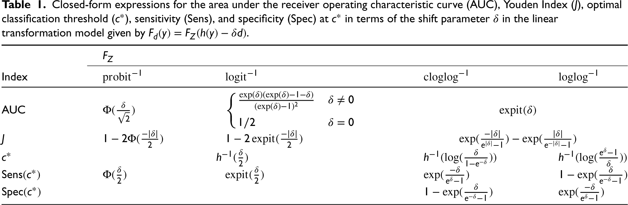
The model assumption implies that a monotone function $h$ exists to transform both $Y_1$ and $Y_0$ into the same distribution, $Z\sim F_Z$ separated by a shift parameter, $\delta$ . The induced ROC curve from this model does not assume a particular distribution of the test result, rather, it quantifies the difference between the test result distributions on the scale of a user-defined $F_Z$ . In this sense, the difference between the test result distributions is described by $\delta$ . Each choice of $F_Z$ leads to a different interpretation of $\delta$ . For example, when $F_Z$ is selected to be the standard normal distribution function, $\delta$ is essentially Cohen’s d, the standardized difference in means of the transformed test results comparing the diseased and nondiseased groups, $\mathbb{E}[h(Y_1)-h(Y_0)]$ . Similarly, when $F_Z$ is the standard logistic distribution function, $\exp (\delta )$ is the ratio of odds of having a positive test result comparing diseased and nondiseased groups. Closed-form expressions can be derived for summary indices of the ROC curve by solving the appropriate integrals. The expressions of AUC, $J$ , the optimal threshold $c^{*}$ , sensitivity and specificity at $c^{*}$ are given for some choices of $F_Z$ in Table 1.

Table 1.

Closed-form expressions for the area under the receiver operating characteristic curve (AUC), Youden Index ( $J$ ), optimal classification threshold ( $c^{*}$ ), sensitivity ( $\text{Sens}$ ), and specificity ( $\text{Spec}$ ) at $c^{*}$ in terms of the shift parameter $\delta$ in the linear transformation model given by $F_d(y)=F_Z(h(y)-\delta d)$ .

	$F_Z$
Index	${\mathrm{probit}}^{-1}$	${\mathrm{logit}}^{-1}$	${\mathrm{cloglog}}^{-1}$	${\mathrm{loglog}}^{-1}$
$\text{AUC}$	$\mathrm{\Phi }(\frac{\delta }{\sqrt{2}})$	$\{\begin{array}{ll}\frac{\exp (\delta )(\exp (\delta )-1-\delta )}{(\exp (\delta )-1{)}^2}& \delta \ne 0\\ 1/2& \delta =0\end{array}$	$\mathrm{expit}(\delta )$
$J$	$1-2\mathrm{\Phi }(\frac{-|\delta |}{2})$	$1-2\mathrm{expit}(\frac{-|\delta |}{2})$	$\exp (\frac{-|\delta |}{e^{|\delta |}-1})-\exp (\frac{|\delta |}{e^{-|\delta |}-1})$
$c^{*}$	$h^{-1}(\frac{\delta }{2})$		$h^{-1}(\log (\frac{\delta }{1-e^{-\delta }}))$	$h^{-1}(\log (\frac{e^{\delta }-1}{\delta }))$
$\text{Sens}(c^{*})$	$\mathrm{\Phi }(\frac{\delta }{2})$	$\mathrm{expit}(\frac{\delta }{2})$	$\exp (\frac{-\delta }{e^{\delta }-1})$	$1-\exp (\frac{\delta }{e^{-\delta }-1})$
$\text{Spec}(c^{*})$			$1-\exp (\frac{\delta }{e^{-\delta }-1})$	$\exp (\frac{-\delta }{e^{\delta }-1})$

2.1.2. Conditional ROC curve

The accuracy of a diagnostic test may be influenced by a set of covariates $\mathit{X}$ . To evaluate their effect on the ROC curve and its summary indices, we assume a linear transformation model with a shift term that takes the form

$${\mu }_d(\mathit{x})=\delta d+{\mathit{x}}^{\mathrm{\top }}\mathit{\xi }+d{\mathit{x}}^{\mathrm{\top }}\mathit{\gamma }$$

(5)

where $\mathit{\xi },\mathit{\gamma }\in {\mathbb{R}}^P$ are the coefficient vectors for the covariates and interaction term, respectively. Under this model, the resulting covariate-specific ROC curve is

$$\text{ROC}(p\mid \mathit{x})=1-F_Z(F_Z^{-1}(1-p)-(\delta +{\mathit{x}}^{\mathrm{\top }}\mathit{\gamma }))$$

where the covariate effect on the ROC curve is given by the difference in shift terms between diseased and nondiseased subjects, $\delta (\mathit{x})=\delta +{\mathit{x}}^{\mathrm{\top }}\mathit{\gamma }$ . Similarly, the covariate-specific AUC is given by

$$\text{AUC}(\mathit{x})=\mathbb{P}(Y_0<Y_1\mid \mathit{X}=\mathit{x})=a(\delta (\mathit{x}))=a(\delta +{\mathit{x}}^{\mathrm{\top }}\mathit{\gamma })$$

(6)

where $a:\mathbb{R}\mapsto [0,1]$ is the AUC function from the first row of Table 1 for different choices of $F_Z$ . The expressions for $J$ , $c^{*}$ , sensitivity and specificity can analogously be adjusted to account for covariates, with $\delta$ replaced by $\delta +{\mathit{x}}^{\mathrm{\top }}\mathit{\gamma }$ in Table 1. In the case of a single continuous covariate $X=x\in \mathbb{R}$ , the interpretation of the interaction coefficient is as follows. For each possible specificity value, a unit increase in $x$ results in a $\gamma$ -unit increase in the ROC curve (or an increase in the sensitivity) on the scale of $F_Z$ . If $\gamma$ is positive, an increase in $x$ corresponds to an increase in the ROC curve, indicating that a test is better able to discriminate the two populations for larger values of $x$ and, vice versa. Note that the ROC curve varies with the covariate contingent upon the presence of an interaction between $d$ and $x$ . For $\gamma =0$ , the covariate affects the distribution of the test results from the diseased and nondiseased population, but not the ROC curve. That is, for all levels of $x$ , the difference between the transformed distributions $h(Y_1)$ and $h(Y_0)$ is given by $\delta$ and the ROC curve is unchanged. Analogous interpretations hold when we are interested in modeling a set of covariates $\mathit{X}$ , which could possibly include categorical covariates.

Standard regression techniques have also been proposed as an alternative to assess the effect of covariates on summary indices rather than deriving the induced ROC curve. For example, Dodd et al. ³² model the partial AUC as a regression function of covariates. Our model equivalently results in a regression model for the AUC, where $\delta +{\mathit{x}}^{\mathrm{\top }}\mathit{\gamma }$ is in the form of a usual linear predictor and $a$ is a monotonically increasing inverse link function which defines the scale for the regression coefficients. As will be shown in Section 2.2, an advantage of our approach is that we do not rely on less efficient binary regression techniques and directly estimate the regression parameters of the transformation model using maximum likelihood estimation. In Supplemental Material Section A, we show that our method is additionally related to the probabilistic index model (PIM) of Thas et al.^33,34

We can also consider more general and potentially nonlinear formulations of the shift and scale terms in our framework. For the special case of $F_Z={\mathrm{probit}}^{-1}$ , the AUC from a shift-scale transformation model ³¹ is given by

$$\mathbb{P}(Y_0<Y_1\mid {\mathit{X}}_0={\mathit{x}}_0,{\mathit{X}}_1={\mathit{x}}_1)=\mathrm{\Phi }\left(\frac{{\mu }_1({\mathit{x}}_1)-{\mu }_0({\mathit{x}}_0)}{{\displaystyle \sqrt{{\sigma }_0({\mathit{x}}_0{)}^2+{\sigma }_1({\mathit{x}}_1{)}^2}}}\right)$$

where ${\mathit{X}}_0$ and ${\mathit{X}}_1$ are the corresponding (potentially different) sets of covariates in the nondiseased and diseased populations, respectively. When the scale term depends only on a single set of covariates, ${\sigma }_0({\mathit{x}}_0)={\sigma }_1({\mathit{x}}_1)=\sigma (\mathit{x})$ , despite varying sets of covariates in the shift terms, all the expressions hold from Table 1 with $\delta$ replaced by $\frac{{\mu }_1({\mathit{x}}_1)-{\mu }_0({\mathit{x}}_0)}{\sigma (\mathit{x})}$ . However, such closed-form expressions cannot be derived for other choices of $F_Z$ when the scale term depends on the disease indicator or on different sets of covariates. In such cases, AUCs and other summary indices can be derived using numerical techniques on the induced ROC curve.

2.2. Estimation

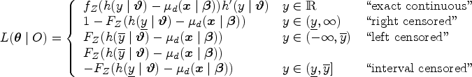
In this section, we propose estimation methods for a transformation model with univariate test results. We provide an explicit parameterization of the transformation function and the shift term. We then maximize the likelihood contributions for a potentially exact continuous, right-, left-, or interval-censored datum to jointly estimate the model parameters. This enables us to fully determine the ROC curve and its summary indices as well as handle test results which are ordinal or impacted by instrument detection limits.

2.2.1. Parameterization

We parameterize the transformation function as

$$h(y\mid \mathit{\vartheta })=\mathit{b}{(y)}^{\mathrm{\top }}\mathit{\vartheta }=\sum _{m=0}^M{\vartheta }_m{b}_m(y)\text{for}y\in \mathbb{R}$$

(7)

where $\mathit{b}(y)=(b_0(y),\dots ,b_M(y){)}^{\mathrm{\top }}$ is a vector of $M+1$ basis functions with coefficients $\mathit{\vartheta }\in {\mathbb{R}}^{M+1}$ . Polynomials in Bernstein form offer a computationally attractive choice of basis that provides a flexible way of estimating the underlying transformation function. The Bernstein basis polynomial of order $M$ is defined on the interval $[l,u]$ as

$$b_m(y)=(\genfrac{}{}{0ex}{}{M}{m}){\tilde{y}}^m(1-\tilde{y}{)}^{M-m},m=0,\dots ,M$$

(8)

where $\tilde{y}=\frac{y-l}{u-l}\in [0,1]$ . The restriction ${\vartheta }_m\le {\vartheta }_{m+1}$ for $m=0,\dots ,M-1$ , guarantees the monotonicity of $h$ . Observe that the transformation function is linear in the parameters that define it and any nonlinearity of the test results is modeled by the basis functions. If the order $M$ is chosen to be sufficiently large, Bernstein polynomials can uniformly approximate any real-valued continuous function on an interval. ³⁵

2.2.2. Likelihood

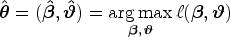
Denote the complete parameter vector as $\mathit{\theta }=({\mathit{\beta }}^{\mathrm{\top }},{\mathit{\vartheta }}^{\mathrm{\top }}{)}^{\mathrm{\top }}$ , where $\mathit{\beta }=(\delta ,{\mathit{\xi }}^{\mathrm{\top }},{\mathit{\gamma }}^{\mathrm{\top }}{)}^{\mathrm{\top }}\in {\mathbb{R}}^{2P+1}$ are the vector of regression coefficients parameterizing the function ${\mu }_d$ from Section 2.1 and $\mathit{\vartheta }\in {\mathbb{R}}^{M+1}$ are the basis coefficients. We follow the maximum likelihood approach proposed by Hothorn et al. ¹³ to jointly estimate $\mathit{\beta }$ and $\mathit{\vartheta }$ . The advantages of embedding the model in the likelihood framework are as follows. (i) All forms of random censoring (right, left, and interval) as well as truncation can directly be incorporated into likelihood contributions defined in terms of the distribution function. ³⁶ Supplemental Material Section A details how ordinal biomarkers can be accommodated in the proposed modeling framework using interval-censored likelihood contributions. (ii) If the given model is correctly specified, under regularity conditions, the maximum likelihood estimator (MLE) will be asymptotically the most efficient estimator. (iii) The MLE is asymptotically normally distributed and has a sample variance that can be computed from the inverse of the Fisher information matrix. This can be used to generate confidence intervals (CIs) for the estimated parameters. (iv) The MLE is equivariant which implies invariance of the score test (or the Lagrange multiplier test) to reparameterizations.^37,38 Specifically, we will show in Section 2.3.1, by inverting the score test, our method produces confidence bands for the ROC curve and appropriate score intervals for its summary indices.

The likelihood contribution of a single observation $O=(Y,D,\mathit{X})$ , where $Y\in (\underset{\_}{y},\overline{y}]=\{y\in \mathbb{R}:\underset{\_}{y}<y\le \overline{y}\}$ is given by

$$\begin{array}{r}L(\mathit{\theta }\mid O)=\{\begin{array}{lll}{f}_Z(h(y\mid \mathit{\vartheta })-{\mu }_d(\mathit{x}\mid \mathit{\beta }))h^{\prime }(y\mid \mathit{\vartheta })& y\in \mathbb{R}& \text{``exact continuous''}\\ 1-F_Z(h(\underset{\_}{y}\mid \mathit{\vartheta })-{\mu }_d(\mathit{x}\mid \mathit{\beta }))& y\in (\underset{\_}{y},\mathrm{\infty })& \text{``right censored''}\\ F_Z(h(\overline{y}\mid \mathit{\vartheta })-{\mu }_d(\mathit{x}\mid \mathit{\beta }))& y\in (-\mathrm{\infty },\overline{y})& \text{``left censored''}\\ F_Z(h(\overline{y}\mid \mathit{\vartheta })-{\mu }_d(\mathit{x}\mid \mathit{\beta }))\\ -F_Z(h(\underset{\_}{y}\mid \mathit{\vartheta })-{\mu }_d(\mathit{x}\mid \mathit{\beta }))& y\in (\underset{\_}{y},\overline{y}]& \text{``intervalcensored''}\end{array}\end{array}$$

where $f_Z$ is the density function of $Z$ and $h^{\prime }(y\mid \mathit{\vartheta })$ is the first derivative of the transformation function with respect to $y$ . Given a sample of $N$ independent and identically distributed observations $O_i$ for $i=1,\dots ,N$ , the log-likelihood is given by $\ell (\mathit{\theta })=\sum _{i=1}^N\log (L_i(\mathit{\theta }))$ , where $L_i$ is the likelihood contribution of observation $i$ . The (unconditional) maximum likelihood estimate of $\mathit{\theta }$ is the solution to the optimization problem

$$\hat{\mathit{\theta }}=(\hat{\mathit{\beta }},\hat{\mathit{\vartheta }})=\underset{\mathit{\beta },\mathit{\vartheta }}{\arg \max }\ell (\mathit{\beta },\mathit{\vartheta })$$

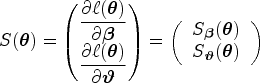
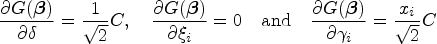
subject to the monotonicity constraint ${\vartheta }_m\le {\vartheta }_{m+1}$ for $m=0,\dots ,M-1$ . The resulting ROC curve only depends on $\mathit{\beta }$ which is decoupled from the parameters needed to model the transformation function $\mathit{\vartheta }$ . The score function is defined as the first derivative of the log-likelihood function with respect to each of the parameters and is given by

$$\begin{array}{r}S(\mathit{\theta })=\left(\begin{array}{l}{\displaystyle \frac{\mathrm{\partial }\ell (\mathit{\theta })}{\mathrm{\partial }\mathit{\beta }}}\\ {\displaystyle \frac{\mathrm{\partial }\ell (\mathit{\theta })}{\mathrm{\partial }\mathit{\vartheta }}}\end{array}\right)=\left(\begin{array}{l}{S}_{\mathit{\beta }}(\mathit{\theta })\\ S_{\mathit{\vartheta }}(\mathit{\theta })\end{array}\right)\end{array}$$

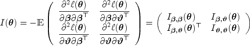
We perform constrained optimization using the likelihood and score contributions to determine the maximum likelihood estimates for $\mathit{\beta }$ and $\mathit{\vartheta }$ (for computational details, see Hothorn ³⁹ ). The asymptotic variance of the MLE can further be estimated by the expected Fisher information matrix which is the variance-covariance matrix of the score function and is defined as

$$\begin{array}{r}I(\mathit{\theta })=-\mathbb{E}\left(\begin{array}{ll}{\displaystyle \frac{{\mathrm{\partial }}^2\ell (\mathit{\theta })}{\mathrm{\partial }\mathit{\beta }\mathrm{\partial }{\mathit{\beta }}^{\mathrm{\top }}}}& {\displaystyle \frac{{\mathrm{\partial }}^2\ell (\mathit{\theta })}{\mathrm{\partial }\mathit{\beta }\mathrm{\partial }{\mathit{\vartheta }}^{\mathrm{\top }}}}\\ {\displaystyle \frac{{\mathrm{\partial }}^2\ell (\mathit{\theta })}{\mathrm{\partial }\mathit{\vartheta }\mathrm{\partial }{\mathit{\beta }}^{\mathrm{\top }}}}& {\displaystyle \frac{{\mathrm{\partial }}^2\ell (\mathit{\theta })}{\mathrm{\partial }\mathit{\vartheta }\mathrm{\partial }{\mathit{\vartheta }}^{\mathrm{\top }}}}\end{array}\right)=\left(\begin{array}{ll}{I}_{\mathit{\beta },\mathit{\beta }}(\mathit{\theta })& I_{\mathit{\beta },\mathit{\vartheta }}(\mathit{\theta })\\ I_{\mathit{\beta },\mathit{\vartheta }}(\mathit{\theta }{)}^{\mathrm{\top }}& I_{\mathit{\vartheta },\mathit{\vartheta }}(\mathit{\theta })\end{array}\right)\end{array}$$

The matrix is partitioned such that the submatrix $I_{\mathit{\beta },\mathit{\beta }}(\mathit{\theta })$ corresponds to the parameter related to the disease indicator and covariates.

2.2.3. Limit of detection

Instrument precision can affect the evaluation of diagnostic biomarkers. For example, when biomarker levels are at or below the limit of detection (LOD) $y_{\text{LOD}}$ , the observed value lies in an interval $(-\mathrm{\infty },y_{\text{LOD}})$ and the resulting measurement is left censored. Often a replacement value is substituted for such measurements. Alternatively, only biomarker values above the LOD are used for the ROC analysis. It has been shown that these approaches lead to biased estimation. ⁴⁰ Various adjustments to ROC curves and its summary indices have been proposed to handle such censored measurements.^41,6,42 However, these methods typically do not account for covariates. Our framework naturally accounts for such observations in the likelihood function for left censored test results. Similarly, the right censored likelihood accounts for measurements which are affected by an upper limit of detection. Thus, our method provides a smooth covariate-specific ROC curve for all values of specificity with estimates and inference appropriately incorporating the observed information.

2.3. Confidence intervals

In the following section, we present three methods to calculate confidence bands for the ROC curve and CIs for its summary indices. Since these quantities are functions $G:{\mathbb{R}}^{2P+1}\to \mathbb{R}$ of the regression parameters $\mathit{\beta }$ in the model, to maintain nominal coverage for a CI for $G(\mathit{\beta })$ , appropriate methods are needed. The methods discussed include inverting the score test, the multivariate delta method and simulation from the asymptotic distribution of the estimate. The methods are ordered by their degree of theoretical justification. We start with score intervals which are invariant to parameter transformations but become computationally expensive when dealing with a large set of parameters. We then discuss estimating the variance using the delta method and conclude with a simple simulation method which is versatile without being computationally demanding.

2.3.1. Score intervals

In the two-sample univariate case where $\delta$ defines the ROC curve, as in equation (5), we can construct score intervals for $\delta$ . Unlike the Wald and other commonly used intervals, score intervals are especially desirable as they are invariant to transformations of the parameters. A score CI for $G(\delta )$ (e.g. the AUC $a(\delta )$ ), provides the same level of coverage as would a score CI for $\delta$ . In turn, under a correctly specified model, a score CI for $\delta$ allows the construction of accurately covered uniform confidence bands for the ROC curve as well as intervals for its summary indices such as the AUC and the Youden index.

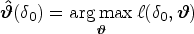
We first generate score CIs for $\delta$ by inverting the score test. In this case, the null hypothesis is given by $H_0:\delta ={\delta }_0$ where ${\delta }_0$ is a specific value of the parameter of interest. Under $H_0$ , the restricted (conditional) MLE for $\mathit{\vartheta }$ can be obtained by

$$\hat{\mathit{\vartheta }}({\delta }_0)=\underset{\mathit{\vartheta }}{\arg \max }\ell ({\delta }_0,\mathit{\vartheta })$$

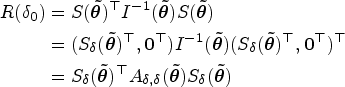
or as a solution of the $M+1$ score equations $S_{\mathit{\vartheta }}({\delta }_0,\mathit{\vartheta })=\mathbf{0}$ . Note that this estimate is a function of ${\delta }_0$ . Letting $\stackrel{\mathbf{~}}{\mathit{\theta }}=({\delta }_0,\hat{\mathit{\vartheta }}({\delta }_0))$ , the quadratic (Rao) score statistic simplifies to

$$\begin{array}{rl}R({\delta }_0)& =S(\stackrel{\mathbf{~}}{\mathit{\theta }}{)}^{\mathrm{\top }}{I}^{-1}(\stackrel{\mathbf{~}}{\mathit{\theta }})S(\stackrel{\mathbf{~}}{\mathit{\theta }})\\ & =(S_{\delta }(\stackrel{\mathbf{~}}{\mathit{\theta }}{)}^{\mathrm{\top }},{\mathbf{0}}^{\mathrm{\top }})I^{-1}(\stackrel{\mathbf{~}}{\mathit{\theta }})(S_{\delta }(\stackrel{\mathbf{~}}{\mathit{\theta }}{)}^{\mathrm{\top }},{\mathbf{0}}^{\mathrm{\top }}{)}^{\mathrm{\top }}\\ & =S_{\delta }(\stackrel{\mathbf{~}}{\mathit{\theta }}{)}^{\mathrm{\top }}{A}_{\delta ,\delta }(\stackrel{\mathbf{~}}{\mathit{\theta }})S_{\delta }(\stackrel{\mathbf{~}}{\mathit{\theta }})\end{array}$$

where $A_{\delta ,\delta }(\stackrel{\mathbf{~}}{\mathit{\theta }})$ denotes the submatrix corresponding to $\delta$ of the inverse Fisher information matrix and is given by the Schur complement $I_{\delta ,\delta }(\mathit{\theta })-I_{\delta ,\mathit{\vartheta }}(\mathit{\theta })I_{\mathit{\vartheta },\mathit{\vartheta }}^{-1}(\mathit{\theta })I_{\delta ,\mathit{\vartheta }}(\mathit{\theta }{)}^{\mathrm{\top }}$ . Under $H_0$ , $R({\delta }_0)$ converges asymptotically to a chi-square distribution with 1 degree of freedom, $R({\delta }_0)\stackrel{D}{⟶}{\chi }_1^2$ . This result is explained by Rao. ⁴³ Inverting the score statistic by enumerating values of ${\delta }_0$ allows for the construction of $(1-\alpha )$ score CIs for $\delta$ defined as

$$\{{\delta }_0\in \mathbb{R}\mid R({\delta }_0)<{\chi }_1^2(1-\alpha )\}$$

where ${\chi }_1^2(1-\alpha )$ is the $(1-\alpha )$ quantile value of the chi-squared distribution with 1 degree of freedom. Equivalently, we can use the square root of the score statistic to construct a $(1-\alpha )$ score interval using quantiles of the standard normal distribution, $\{{\delta }_0\in \mathbb{R}\mid {\mathrm{\Phi }}^{-1}(\alpha /2)<\sqrt{R({\delta }_0)}\le {\mathrm{\Phi }}^{-1}(1-\alpha /2)\}$ . Finally, we apply the function $G$ to both the lower and upper limits of the interval to construct score confidence bands for the ROC curve or score CIs for its summary indices.

The score statistic is given by $R({\delta }_0)=S_{\delta }(\stackrel{\mathbf{~}}{\mathit{\theta }}{)}^2{A}_{\delta ,\delta }(\stackrel{\mathbf{~}}{\mathit{\theta }})$ . Testing if there is a significant difference between the nondiseased and diseased populations coincides to the hypothesis test, $H_0:\delta =0$ . This is computationally efficient because only the distribution of $R(0)$ needs to be computed. However, computing score CIs for more than one parameter requires updating the restricted MLEs $\hat{\mathit{\vartheta }}({\delta }_0)$ for an enumeration of ${\delta }_0$ values. This becomes computationally intractable when enumerating a higher-dimensional grid of parameters.

2.3.2. Delta method

Since the MLE satisfies

$$\sqrt{n}(\hat{\mathit{\beta }}-\mathit{\beta })\stackrel{D}{\to }{N}_{P+1}(\mathbf{0},A_{\mathit{\beta },\mathit{\beta }}(\mathit{\theta }))$$

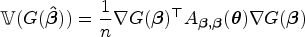
then by the multivariate delta method, $G(\hat{\mathit{\beta }})$ also follows a normal distribution with

$$\mathbb{V}(G(\hat{\mathit{\beta }}))=\frac{1}{n}\mathrm{\nabla }G(\mathit{\beta }{)}^{\mathrm{\top }}{A}_{\mathit{\beta },\mathit{\beta }}(\mathit{\theta })\mathrm{\nabla }G(\mathit{\beta })$$

where $\mathrm{\nabla }G(\mathit{\beta })$ is the gradient of $G$ evaluated at $\mathit{\beta }$ and the inverse Fisher information matrix $A_{\mathit{\beta },\mathit{\beta }}(\mathit{\theta })$ is given by the Schur complement $I_{\mathit{\beta },\mathit{\beta }}(\mathit{\theta })-I_{\mathit{\beta },\mathit{\vartheta }}(\mathit{\theta })I_{\mathit{\vartheta },\mathit{\vartheta }}^{-1}(\mathit{\theta })I_{\mathit{\beta },\mathit{\vartheta }}(\mathit{\theta }{)}^{\mathrm{\top }}$ . For example, when the shift term takes the linear form as in equation (6) and $G$ defines the AUC function for $F_Z={\mathrm{probit}}^{-1}$ , the entries of $\mathrm{\nabla }G(\mathit{\beta })$ are given by

$$\frac{\mathrm{\partial }G(\mathit{\beta })}{\mathrm{\partial }\delta }=\frac{1}{\sqrt{2}}C,\frac{\mathrm{\partial }G(\mathit{\beta })}{\mathrm{\partial }{\xi }_i}=0\text{and}\frac{\mathrm{\partial }G(\mathit{\beta })}{\mathrm{\partial }{\gamma }_i}=\frac{x_i}{\sqrt{2}}C$$

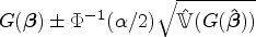
where $C=\varphi (\frac{\delta +{\mathit{x}}^{\mathrm{\top }}\mathit{\gamma }}{\sqrt{2}})$ , $\varphi$ is the density of the standard normal distribution and $i$ indexes the $P$ covariates. In general, the gradient can be estimated by calculating such derivatives and evaluating the resulting function at the MLE. Similarly, the variance-covariance matrix of the estimated parameters $A_{\mathit{\beta },\mathit{\beta }}(\mathit{\theta })$ can be computed by inverting the numerically evaluated Hessian matrix. Thus, a $(1-\alpha )$ level CI for $G(\mathit{\beta })$ is given by

$$G(\mathit{\beta })\pm {\mathrm{\Phi }}^{-1}(\alpha /2)\sqrt{\hat{\mathbb{V}}(G(\hat{\mathit{\beta }}))}$$

2.3.3. Simulated intervals

When the function $G$ has complex derivatives, as would be the case for nonlinear shift terms ${\mu }_d(\mathit{x})$ or when calculating optimal thresholds $c^{*}$ where $G$ includes the inverse of the transformation function, constructing CIs using the delta method becomes infeasible. For these cases, we apply a simple simulation-based algorithm which utilizes the asymptotic normality of the MLE to calculate CIs for the ROC curve and its summary indices, which are functions of the parameters of interest. The steps of the algorithm to construct $(1-\alpha )$ level CIs for $G(\hat{\mathit{\beta }})$ can be summarized as follows:

Generate $B$ independent samples from the asymptotic multivariate normal distribution of the parameter estimates $N_{P+1}(\hat{\mathit{\beta }},\frac{1}{n}{\hat{A}}_{\mathit{\beta },\mathit{\beta }}(\hat{\mathbf{\Theta }}))$ and denote as ${\hat{\mathit{\beta }}}_1^{*},\dots ,{\hat{\mathit{\beta }}}_B^{*}$ .

For each sample $b=1,\dots ,B$ , calculate the function of interest $G({\hat{\mathit{\beta }}}_b^{*})$ .

Construct the CI $(Q_{G({\hat{\mathit{\beta }}}^{*})}(\alpha /2),Q_{G({\hat{\mathit{\beta }}}^{*})}(1-\alpha /2))$ , where $Q_{G({\hat{\mathit{\beta }}}^{*})}$ is the empirical quantile function of the sample $G({\hat{\mathit{\beta }}}_1^{*}),\dots ,G({\hat{\mathit{\beta }}}_B^{*})$ .

A similar algorithm is presented by Mandel, ⁴⁴ who discuss its asymptotic validity and present several examples that show its empirical coverage adheres to nominal levels with results similar to the delta method.

3. Empirical evaluation

We conducted a simulation study to evaluate the performance of our estimators in the two-sample setting. We chose this setting to be able to compare various estimators commonly used in practice. The software details of all the methods used alongside their respective features and references are summarized in Table 2.

Table 2.

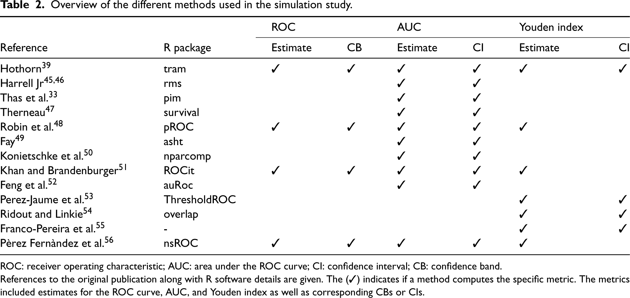
Overview of the different methods used in the simulation study.

		ROC		AUC		Youden index
Reference	R package	Estimate	CB	Estimate	CI	Estimate	CI
Hothorn 39	tram	$✓$	$✓$	$✓$	$✓$	$✓$	$✓$
Harrell Jr45,46	rms			$✓$	$✓$
Thas et al. 33	pim			$✓$	$✓$
Therneau 47	survival			$✓$	$✓$
Robin et al. 48	pROC	$✓$	$✓$	$✓$	$✓$	$✓$
Fay 49	asht			$✓$	$✓$
Konietschke et al. 50	nparcomp			$✓$	$✓$
Khan and Brandenburger 51	ROCit	$✓$	$✓$	$✓$	$✓$	$✓$
Feng et al. 52	auRoc			$✓$	$✓$
Perez-Jaume et al. 53	ThresholdROC					$✓$	$✓$
Ridout and Linkie 54	overlap					$✓$	$✓$
Franco-Pereira et al. 55	-					$✓$	$✓$
Pèrez Fernàndez et al. 56	nsROC	$✓$	$✓$	$✓$	$✓$	$✓$

ROC: receiver operating characteristic; AUC: area under the ROC curve; CI: confidence interval; CB: confidence band.

References to the original publication along with R software details are given. The ( $✓$ ) indicates if a method computes the specific metric. The metrics included estimates for the ROC curve, AUC, and Youden index as well as corresponding CBs or CIs.

We considered a data generating process (DGP) such that nondiseased test results followed a standard normal distribution $F_0(y)=\mathrm{\Phi }(y)$ and the diseased test results a distribution with the CDF $F_1(y)=F_{Z_{\text{DGP}}}(F_{Z_{\text{DGP}}}^{-1}(\mathrm{\Phi }(y))-\delta )$ . To obtain different shapes of the ROC curve, we chose three choices of $F_{Z_{\text{DGP}}}\in \{{\mathrm{probit}}^{-1},{\mathrm{logit}}^{-1},{\mathrm{cloglog}}^{-1}\}$ and varied $\delta$ such that the $\text{AUC}\in \{0.5,0.65,0.8,0.95\}$ or that $J\in \{0,0.25,0.5,0.8\}$ , leading to a variety of configurations. Under this simulation paramaterization, the true ROC curves followed the form of equation (5) and the true summary indices could be calculated as a function of $\delta$ from Table 1.

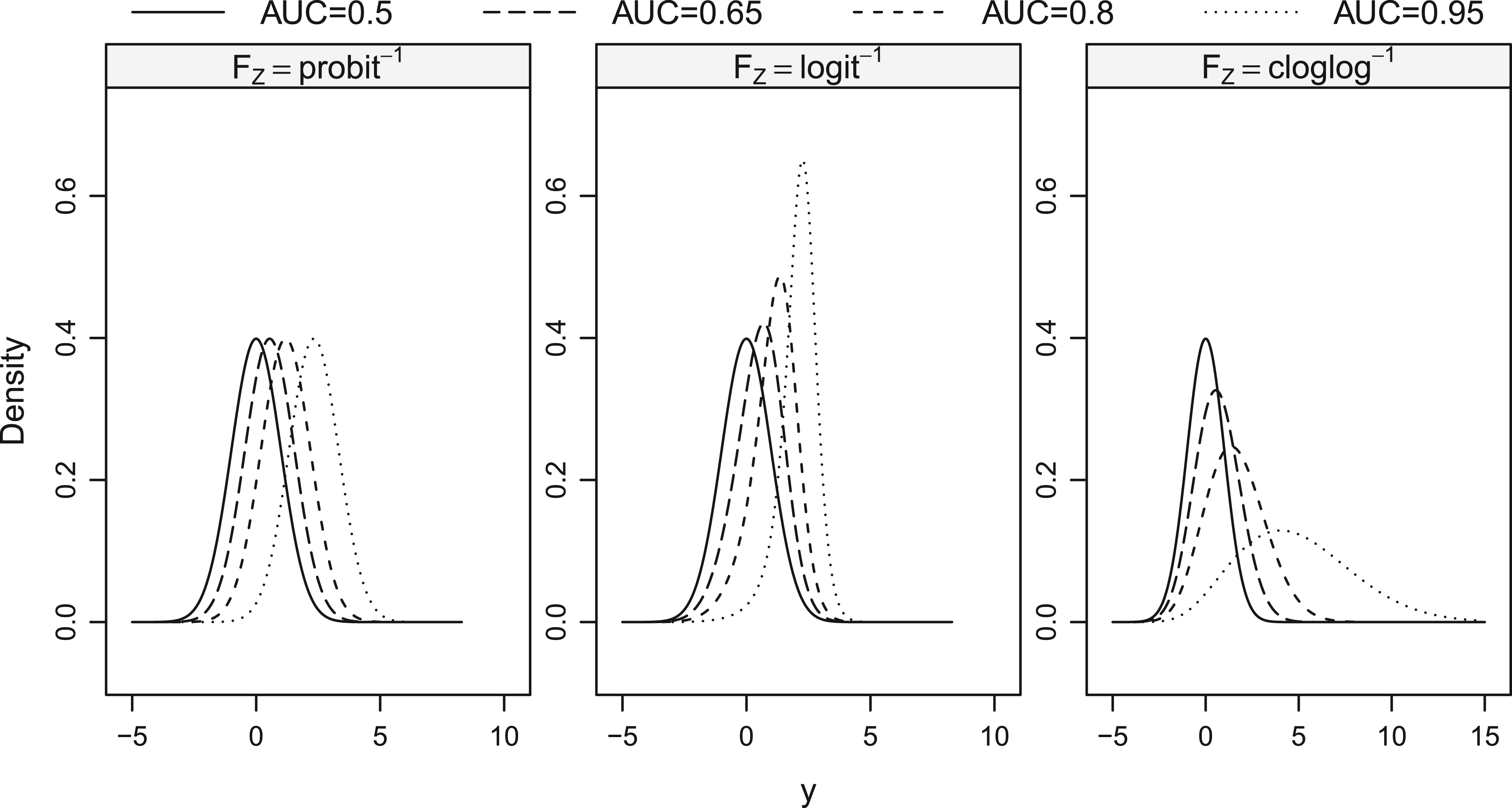
The conventional binormal model corresponded to $F_{Z_{\text{DGP}}}={\mathrm{probit}}^{-1}=\mathrm{\Phi }$ and induced proper binormal ROC curves. This was the only configuration where the test results for both groups were normally distributed. We included this configuration to ascertain the loss of power associated with our estimators when the standard binormal assumption held. For other choices of $F_{Z_{\text{DGP}}}$ with $\text{AUC}>0.5$ , the resulting distributions of the diseased test results were non-normal, with variances and higher moments differing between the two groups. Specifically, the configuration of $F_{Z_{\text{DGP}}}={\mathrm{logit}}^{-1}$ led to light tailed distributions for the diseased test results, while $F_{Z_{\text{DGP}}}={\mathrm{cloglog}}^{-1}$ led to skewed, heavy-tailed distributions. The corresponding density functions for the data generating model with selected AUC values are given in Figure 1.

Figure 1.

Density functions for the model used to generate the data for the simulations. The nondiseased test results followed a standard normal distribution corresponding to an $\text{AUC}=0.5$ . The diseased test results varied with three choices of $F_{Z_{\text{DGP}}}$ : ${\mathrm{probit}}^{-1}$ , ${\mathrm{logit}}^{-1}$ , and ${\mathrm{cloglog}}^{-1}$ each of which had an AUC of 0.5, 0.65, 0.8, and 0.95. DGP: data generating process; AUC: area under the receiver operating characteristic curve.

For 10,000 replications of each configuration, we generated balanced data sets with sample sizes $N_0=N_1\in \{25,50,100\}$ . The transformation models discussed in Section 2 were fitted to the simulated data sets assuming a parameterization of the transformation function given by a Bernstein basis polynomial of order $M=6$ (see Hothorn ³⁹ for a discussion on suitable choices for $M$ ). The true data-generating model had a nonlinear transformation function $h=F_{Z_{\text{DGP}}}^{-1}\circ \mathrm{\Phi }$ . Our model estimation procedure aimed to approximate this function alongside the shift parameter $\delta$ . The functions implementing transformation models for different choices of $F_Z$ are available from the tram add-on package. ³⁹ Note that the function $F_{Z_{\text{DGP}}}$ is for the data generating process in the simulation study and is distinct from $F_Z$ , the inverse link function used in the model. When $F_{Z_{\text{DGP}}}=F_Z$ , the model is correctly specified for the DGP.

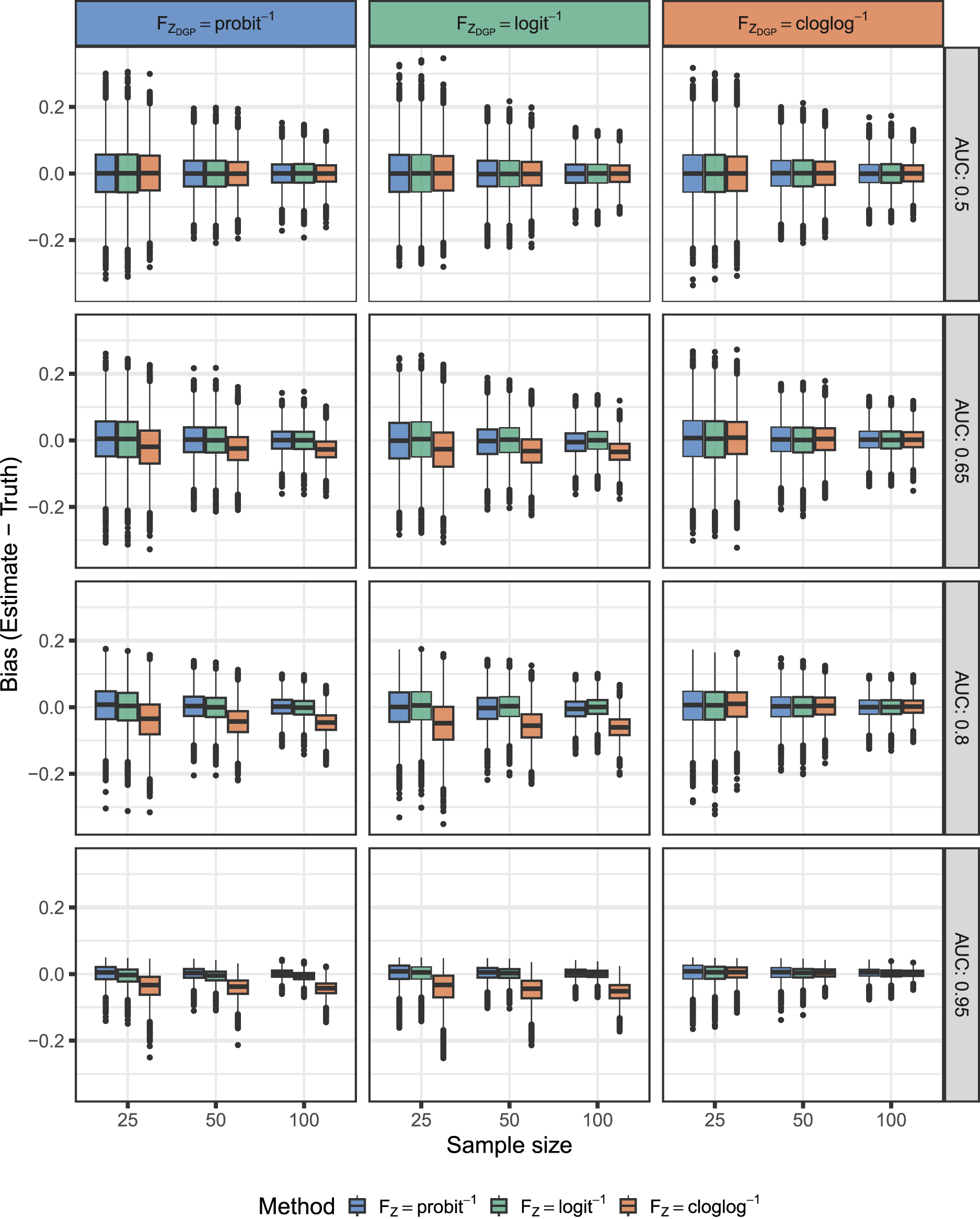
Figure 2 displays the distribution of bias for the AUC estimates using the proposed methods under the various simulation configurations. We found that all three methods had minimal bias for an $\text{AUC}=0.5$ , where the test results were unable to distinguish between the two groups. The models with $F_Z\in \{{\mathrm{probit}}^{-1},{\mathrm{logit}}^{-1}\}$ yielded approximately unbiased AUC estimates in all cases, even when they were misspecified for the true data generating process. However, estimates based on the proportional hazards model $F_Z={\mathrm{cloglog}}^{-1}$ , were biased for data generating processes other than where it was correctly specified.

Figure 2.

Distribution of bias from the simulation study for estimation of the AUC. The DGP for nondiseased results was $F_0(y)=\mathrm{\Phi }(y)$ and for diseased results $F_1(y)=F_{Z_{\text{DGP}}}(F_{Z_{\text{DGP}}}^{-1}(\mathrm{\Phi }(y))-\delta )$ . We varied $F_{Z_{\text{DGP}}}\in \{{\mathrm{probit}}^{-1}$ , ${\mathrm{logit}}^{-1}$ , ${\mathrm{cloglog}}^{-1}\}$ , AUC and sample size. The proposed methods also varied by the same inverse link functions. An alignment of colors in the column (DGP) and the fill of the box plot is indicative that the method is correctly specified for the DGP. DGP: data generating process; AUC: area under the receiver operating characteristic curve.

We compared our approaches to a set of alternative methods (see Table 2) for computing CIs for the AUC and Youden index. We detail the empirical coverage and average width of the CIs for the AUC in Supplemental Figures S1 and S2, respectively. Estimates based on transformation models (R packages tram, orm, pim) yielded coverage close to the nominal level and significantly outperformed the other methods when the model was correctly specified for the true data generating process. All other methods generally performed close to nominal levels for low to medium AUC values (0.5–0.8), but broke down for higher AUC values. In addition, the score CIs from the transformation model with $F_Z={\mathrm{logit}}^{-1}$ were accurate even when it was misspecified for the true data generating process. However, methods which used $F_Z={\mathrm{cloglog}}^{-1}$ gave CIs which were shorter in length (overconfident).

Analogously, Supplemental Figures S3 and S4 detail the coverage and length of the CIs for the Youden index. The methods which were based on the overlap coefficient failed to cover the configuration where $J=0$ because their lower limits were never below 0. Our methods estimated CIs for $\delta \in \mathbb{R}$ which naturally accounted for this scenario. The transformation model with $F_Z={\mathrm{logit}}^{-1}$ provided coverage at nominal levels for all simulation configurations with a relatively small CI width. The approach of Franco-Pereira et al. ⁵⁵ (FP) was also accurate under model misspecification but was more involved. Namely, it consisted of estimating Box-Cox transformation parameters under a binormal framework with bootstrap variance, all carried out on the logit scale and then back-transformed. In a setting with covariates, censoring or with $J=0$ this methodology would be limited.

Supplemental Figures S5 and S6 show the coverage and area of the confidence bands for the ROC curve. All the approaches based on transformation models covered the configuration with $\text{AUC}=0.5$ accurately. However, the other approaches did not yield coverage close to nominal levels in this configuration with the exception of Martínez-Camblor et al., ⁵⁷ whose confidence bands had a significantly larger area indicating lower power. For all other configurations, only transformation models which were correctly specified for the true data-generating model provided accurate results.

In addition to the simulations described above, we considered three other scenarios to evaluate the robustness of our proposed methods to model misspecification. The details for each of these scenarios are given in Supplemental Materials Section B. In terms of the AUC, we noticed that our models are generally robust to misspecification, but can break down in certain cases. However, the proportional hazard model with $F_Z={\mathrm{cloglog}}^{-1}$ resulted in poor performance under misspecified configurations, indicating that it should be used with caution.

4. Application

The prevalence of obesity has increased consistently for most countries in the recent decade and this trend is a serious global health concern. ⁵⁸ Obesity contributes directly to increased risk of cardiovascular disease (CVD) and its risk factors, including type 2 diabetes, hypertension, and dyslipidemia.^59,60 Metabolic syndrome (MetS) refers to the joint presence of several cardiovascular risk factors and is characterized by insulin resistance. ⁶¹ The National Cholesterol Education Program Adult Treatment Panel III (NCEP-ATP III) criteria is the most widely used definition for MetS, but it requires laboratory analysis of a blood sample. This has led to the search for non-invasive techniques which allow reliable and early detection of MetS.

Waist-to-height ratio (WHtR) is a well-known anthropometric index used to predict visceral obesity. Visceral obesity is an independent risk factor for development of MetS by means of the increased production of free fatty acids whose presence obstructs insulin activity. ⁶² This suggests that higher values of WHtR, reflecting obesity, and CVD risk factors, are more indicative of incident MetS. Several studies have found that WHtR is highly predictive of MetS.^63–65 However, as waist circumference changes with age and gender, ⁶⁶ it is also important to study whether or not the performance of WHtR at diagnosing MetS is impacted by these variables. Evaluation of WHtR as a predictor of MetS after adjusting for covariates is necessary so that more tailored interventions can be initiated to improve outcomes.

We illustrate the use of our methods to data from a cross sectional study designed to validate the use of WHtR and systolic blood pressure (SBP) as markers for early detection of MetS in a working population from the Balearic Islands (Spain). Detailed descriptions of the study methodology and population characteristics are reported in Romero-Saldaña et al. ⁶⁷ Briefly, data on 60 799 workers were collected during their work health periodic assessments between 2012 and 2016. Presence of MetS was determined by the NCEP-ATP III criteria and the sample consisted of 5487 workers with MetS.

4.1. Two-sample analysis

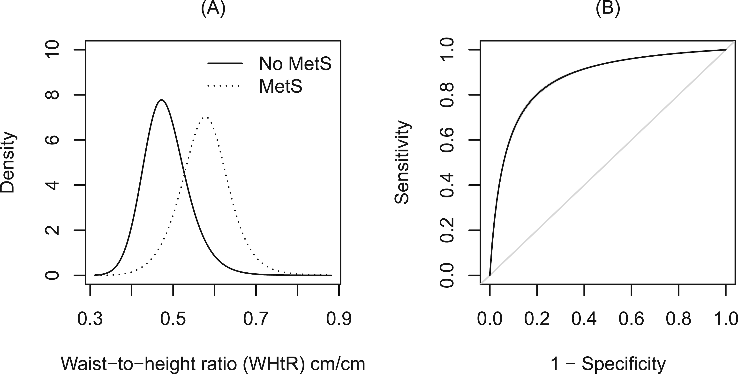
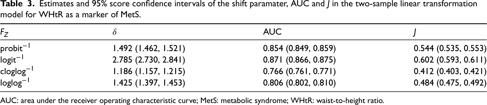
We first examined the unconditional performance of WHtR as a marker to diagnose MetS, denoted $Y$ and $D$ , respectively. We fitted a linear transformation model with corresponding ROC curve of the form in equation (5), where $\delta$ is the shift parameter, for various choices of the inverse link function $F_Z$ . Associated inference of the AUC and $J$ was calculated using the closed-form expressions from Table 1. The resulting estimates are presented in Table 3. The AUCs were consistently bounded away from $0.5$ indicating a good capacity of WHtR to discriminate between workers with and without MetS. This can also be seen from the estimated ROC curve plotted in Figure 3 which lies well above the diagonal line as well as the modeled densities which have a small degree of overlap. The CIs and uniform confidence bands were quite small due to the large sample size.

Figure 3.

Estimates from the linear transformation model with a single shift parameter, $h(Y)=\delta d+Z$ , where $Z$ is chosen to be a standard logistic distribution. (A) Density functions of WHtR for the workers who were diagnosed with MetS (dotted line) and those who were not (solid line). (B) ROC curve for WHtR as a marker of MetS with 95% uniform score confidence bands are represented by gray shaded areas. MetS: metabolic syndrome; WHtR: waist-to-height ratio.

Table 3.

Estimates and 95% score confidence intervals of the shift paramater, AUC and $J$ in the two-sample linear transformation model for WHtR as a marker of MetS.

$F_Z$	$\delta$	AUC	$J$
${\text{probit}}^{-1}$	1.492 (1.462, 1.521)	0.854 (0.849, 0.859)	0.544 (0.535, 0.553)
${\text{logit}}^{-1}$	2.785 (2.730, 2.841)	0.871 (0.866, 0.875)	0.602 (0.593, 0.611)
${\text{cloglog}}^{-1}$	1.186 (1.157, 1.215)	0.766 (0.761, 0.771)	0.412 (0.403, 0.421)
${\text{loglog}}^{-1}$	1.425 (1.397, 1.453)	0.806 (0.802, 0.810)	0.484 (0.475, 0.492)

AUC: area under the receiver operating characteristic curve; MetS: metabolic syndrome; WHtR: waist-to-height ratio.

4.2. Conditional ROC analysis

Next, we investigated if the discriminatory ability of WHtR in separating workers with and without MetS varies with covariates. We considered a transformation model that included the main effects of covariates plus interaction terms with the disease indicator, which leads to the ROC curve given by

$$\text{ROC}(p\mid \mathit{x})=1-F_Z(F_Z^{-1}(1-p)-(\delta +{\gamma }^{\mathrm{\top }}\mathit{x}))$$

where the covariates $\mathit{x}$ included age, gender, and tobacco consumption. The choice of $F_Z={\mathrm{logit}}^{-1}$ was made using repeated holdout validation. We describe this model selection procedure in Supplemental Material Section C and show the results for different model choices and parameterizations.

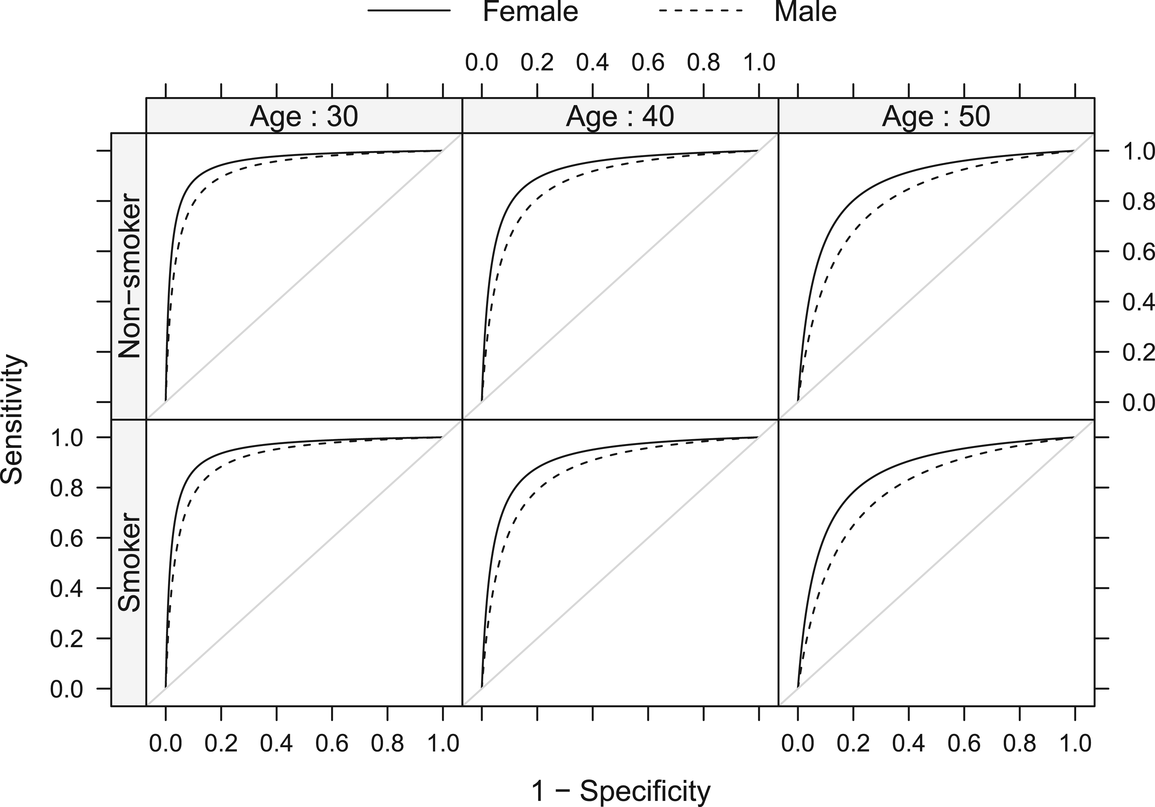
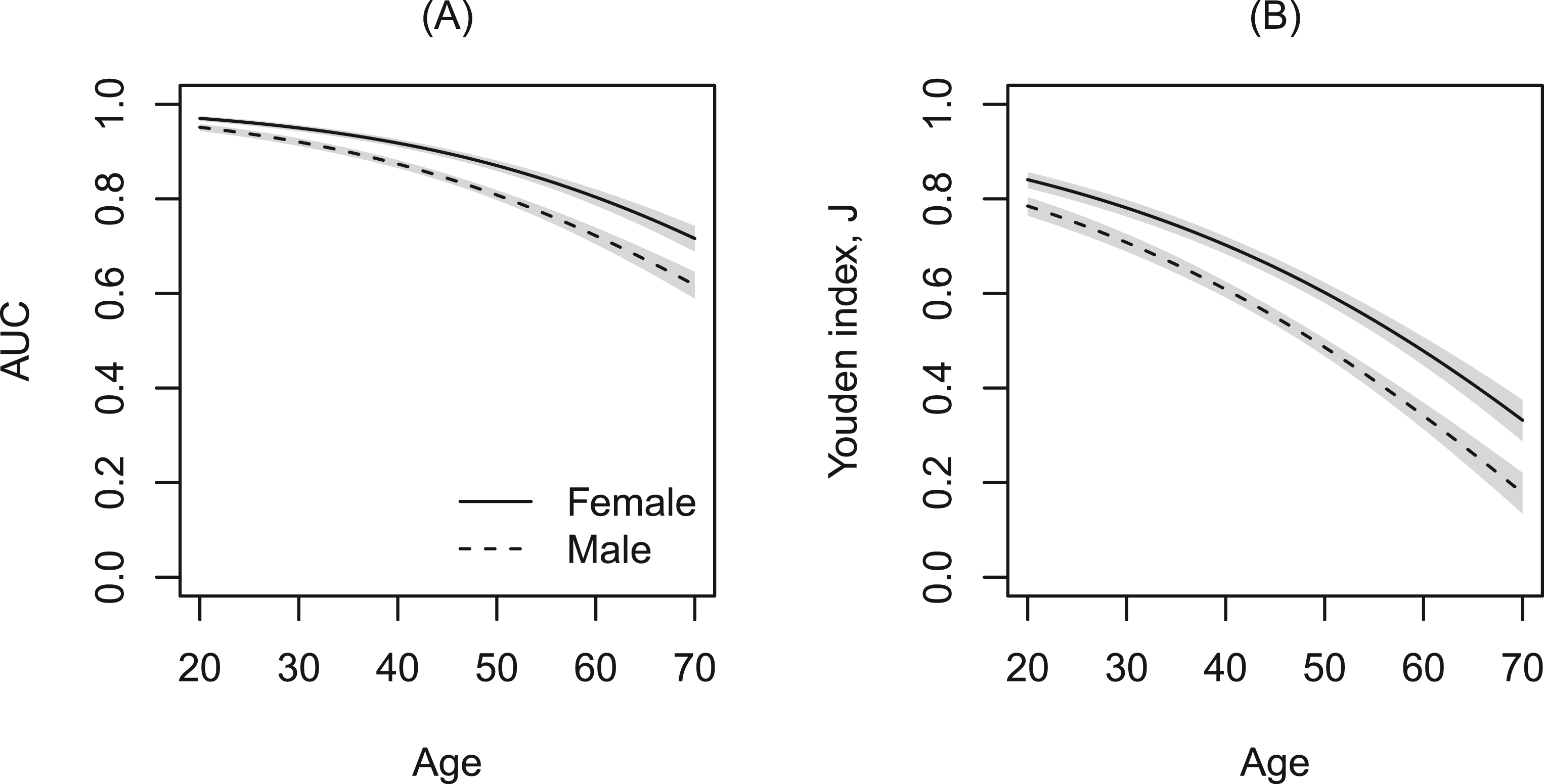
Figure 4 displays the covariate-specific ROC curves fitted to these data. The performance of WHtR appeared to be better for females compared to males and decreased with age. The effect of smoking, although significant in the model, does not seem to substantially alter the ROC curves given the other covariates are kept fixed. To inspect the covariate effect further, we calculated the age- and gender-specific AUCs and Youden indices from the model. Figure 5 clearly shows that the discriminatory capabilities of WHtR in distinguishing workers with MetS is consistently better for females and decreases with age.

Figure 4.

Estimated covariate-specific ROC curves for WHtR as a marker of MetS for female (solid line) and male workers (dashed line). Vertical panels represent a specific age (30, 40, 50) and horizontal panels smoking status. ROC: receiver operating characteristic; MetS: metabolic syndrome; WHtR: waist-to-height ratio.

Figure 5.

Age-based AUC and Youden indices where WHtR is used as a marker to detect MetS for non-smoking female (solid line) and male (dashed line) workers. 95% Wald pointwise confidence bands are represented by gray shaded areas. AUC: area under the receiver operating characteristic curve; MetS: metabolic syndrome; WHtR: waist-to-height ratio.

5. Discussion

This article presents a new modeling framework for ROC analysis that can be used to characterize the accuracy of medical diagnostic tests. Our model is based on estimating an unknown transformation function for the test results and yields a distribution-free yet model-based estimator for the ROC curve. Covariates that influence the diagnostic accuracy of tests can naturally be accommodated as regression parameters into the model and covariate-specific summary indices such as the AUC and Youden index are easily computed using closed-form expressions.

Our proposed approach has several features which distinguish it from contemporary methods of ROC analysis. Firstly, we employ maximum likelihood to jointly estimate all parameters defining the transformation function and regression coefficients. This implies the variation in the estimated transformation parameters is accounted for and appropriately propagated to inference for the ROC curve. In turn, asymptotic efficiency is guaranteed for our estimators and we avoid reliance on resampling procedures for the construction of CIs. Secondly, transformation models focus on estimating the conditional distribution function whose evaluation directly provides the likelihood contributions for interval, right-, and left-censored data that commonly arises due to instrument detection limits. Thirdly, no strong assumptions are made regarding the transformation function which results in a highly flexible model that retains interpretability of the regression coefficients. Lastly, software implementations for all the methods described in this article are available in the tram R add-on package (see Supplemental Material for example code), thus enabling a unified framework for ROC analysis.

In our simulation study, interestingly, we found that a model with $F_Z={\mathrm{logit}}^{-1}$ provided accurate results even when it was misspecified for the true data generating process. This model also behaves very similarly to the semiparametric cumulative probability model, ⁶⁸ both of which estimate a log-odds ratio $\delta$ . The equivalence of the transformation model’s odds ratio to the MWW test statistic has been well studied. ⁶⁹ The MWW statistic has a bounded influence function and is robust to contaminations of the specified model. ⁷⁰ Due to their equivalence, we hypothesize that the transformation model with $F_Z={\mathrm{logit}}^{-1}$ is also endowed with the same robustness properties as the MWW and thus can be chosen when no a priori model is known.

One aspect that warrants further investigation is model selection, specifically with regards to the choice of $F_Z$ . One strategy would be to define $F_Z$ tailored to a specific interpretation of the parameters $\delta$ , $\mathit{\beta }$ , and $\mathit{\gamma }$ , for example, as log-odds ratios with $F_Z={\mathrm{logit}}^{-1}$ or $F_Z={\mathrm{cloglog}}^{-1}$ for hazard ratios. ³⁴ A second option is to use some form of cross validation in combination with model assessment via the probability integral transform (PIT) (as discussed in Supplemental Materials Section C). Third, and in analogy to single index models, one could introduce parameters to $F_Z$ such that the shape of the inverse link function is estimated along with all other model parameters (McLain and Ghosh ⁷¹ discuss a family of link functions including the complementary log-log and logit). Finally, we could completely relax the assumption that the difference between the diseased and nondiseased distributions is described by a shift-term. In this case, separate transformation functions would be allowed in each of the two groups. Namely, consider a stratified model where the nondiseased results follow a distribution with the CDF $F_0(y)=F_Z(h_0(y))$ and the diseased with the CDF $F_1(y)=F_Z(h_1(y))$ . Defining a new transformation function $r=h_1\circ h_0^{-1}\circ F_Z^{-1}:[0,1]\mapsto \mathbb{R}$ , the smooth ROC curve with no shift assumptions is given by $\text{ROC}(p)=1-F_Z(r(1-p))$ . This model has more flexibility but sacrifices the properness property desirable for the ROC curves. Furthermore, care has to be taken in defining the correct likelihood contributions for accurate inference of this model as uncertainty enters from both transformation functions.

In future work, we plan to pursue various extensions of transformation models for ROC analysis to consider (1) penalty terms for high-dimensional covariates, ⁷² (2) mixed effects for clustered observations, ⁷³ and (3) covariate-dependent transformation functions through forest-based machine learning methods. ⁷⁴

Supplemental Material

sj-pdf-1-smm-10.1177_09622802231176030 - Supplemental material for Estimating transformationsfor evaluating diagnostic testswith covariate adjustment

Supplemental material, sj-pdf-1-smm-10.1177_09622802231176030 for Estimating transformationsfor evaluating diagnostic testswith covariate adjustment by Ainesh Sewak and Torsten Hothorn in Statistical Methods in Medical Research