
Abstract
Illness-death models are a class of stochastic models inside the multi-state framework. In those models, individuals are allowed to move over time between different states related to illness and death. They are of special interest when working with non-terminal diseases, as they not only consider the competing risk of death but also allow us to study the progression from illness to death. The intensity of each transition can be modelled including both fixed and random effects of covariates. In particular, spatially structured random effects or their multivariate versions can be used to assess spatial differences between regions and among transitions. We propose a Bayesian methodological framework based on an illness-death model with a multivariate Leroux prior for the random effects. We apply this model to a cohort study regarding progression after an osteoporotic hip fracture in elderly patients. From this spatial illness-death model, we assess the geographical variation in risks, cumulative incidences and transition probabilities related to recurrent hip fracture and death. Bayesian inference is done via the integrated nested Laplace approximation.
Keywords
Introduction
Multi-state models are stochastic models which generalise a wide class of survival scenarios, from unidimensional survival models to multi-event models such as competing risks models or repeated events.1,2 In the multi-state framework, events are the states of the process, and their respective occurrences are transitions between the state of departure and the state of interest. The uncertainty associated with transitions is modelled via transition probabilities or, equivalently, transition intensities. The latter are analogue to hazard functions in the field of survival analysis. Multi-state models are especially useful in medical research because they provide a natural setting for dealing with the natural history of complex diseases. 3
The so-called illness-death model 4 is one of the simplest and most studied multi-state models. It has three states: an initial state, an illness-related state and a death state. The process starts in the initial state from which it can progress to the illness transient state or to death, which is an absorbent state. Death is also accessible from the illness state. This model is particularly useful to the study of chronic diseases, 5 cancer progression 6 or cardiovascular diseases 7 in which there is a considerable risk of death over time.
The Cox proportional hazards model 8 is the most popular regression tool in the survival framework to model hazard functions associated with survival times. It expresses hazard functions as the product of a time-dependent baseline hazard function and the exponential of a regression term including covariates and latent elements. The popularity of this model is primarily due to two reasons. First, due to the interpretability of hazard ratios to evaluate differences in the risk of the event of interest among the different covariate levels. Second, because under the frequentist paradigm, that the objective does not require to make any assumptions about the baseline hazard function. From Bayesian reasoning, a model for the baseline risk function needs to be specified, 9 either parametrically or semi-parametrically. 10 In particular, when we work only with covariates and use a Weibull baseline risk function, the overall risk function will also be Weibull. This property is the basis of the correspondence between the Weibull Cox proportional hazards model and the Weibull accelerated failure time (AFT) regression model. 11
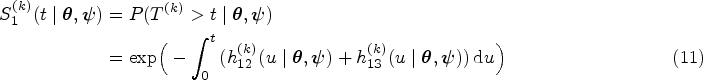
The Bayesian paradigm provides a flexible framework for statistical inferences and the generation of knowledge. Under this framework, any measure of interest is subject to uncertainty: not only random variables but also parameters, hypotheses, models, etc. On the other hand, the Bayesian inferential process via the Bayes’ theorem allows for sequentially updated previous knowledge of those measures using new information. The procedure is conceptually simple: the elicitation of a prior distribution for all uncertainties in the model, the computation of the likelihood function for the data obtained, and the estimation of the posterior distribution which updates the relevant knowledge. This posterior is the starting point to approximate the posterior distribution of any measure of interest, such as sojourn times, transition and occupation probabilities, and cumulative incidence functions.
Regression survival models can include not only covariates but also latent effects that account for some non-explained heterogeneity between groups of the target population. In particular, the existence of differences among spatial regions is especially common in epidemiological studies. Uncontrolled risk factors may be relevant to explain high or low risks of disease in some regions, leading to this heterogeneity. We focus in this article on lattice data, that is, data for a finite number of sub-regions of a larger one. Often neighbouring regions can be expected to be similar and thus random effects with a spatial correlation structure can be assumed.
There are a plenty of models for assessing spatial correlation in the statistical literature. Conditional autoregressive (CAR) models 12 and their variants based on a neighbourhood definition of the correlation have been widely used in disease mapping. In particular, the model proposed by Besag, York and Molliè (BYM) in 1991 13 has been postulated as the main choice over the past decades to deal with counts assuming a Poisson process. It is defined by means of two random effects, the first based on the neighbourhood structure and thus summarizing the spatial correlation between regions, and the second unstructured accounting for heterogeneity among regions. Leroux et al. 14 proposed an alternative specification for the precision matrix of the spatially distributed random effects that better distinguishes between spatial dependence and dispersion effects. Under this model, random effects are defined as a mixture of independent and spatially correlated scenarios. Some authors assessed the behaviour of spatial models inside the survival framework such as Banerjee, Wall and Carlin, 15 comparing different models without random effects (usually referred as frailties in the survival setting), with non-spatial frailties and with a CAR frailty.
Regarding illness-death models, not only spatial correlation can be modelled, but also a correlation between the three transitions, resulting in a multivariate model for random effects. In this regard, Carlin and Banerjee 16 proposed a multivariate CAR model for spatially correlated survival times. However, despite its interest, there are few studies considering spatial components in the illness-death model framework. The most remarkable research work in this direction is Nathoo and Dean 17 in which various structures for region-specific random effects are proposed, with special attention to the comparison of different baseline functions such as Weibull distributions, piecewise-exponential forms and cubic B-splines.
We propose a Bayesian methodological framework to deal with spatially correlated random effects within the illness-death scenario. In particular, a multivariate version of the Leroux model is used to jointly model that spatial correlation as well as the correlation between the transition survival times. The Bayesian procedure involving the approximation of the relevant posterior distribution is done via the integrated nested Laplace approximation (INLA), which in general provides accurate estimations and reduces the computational time compared to Markov chain Monte Carlo (MCMC) methods. In the context of the proposed methodological framework, the computation of posterior outcomes such as sojourn times, transition and occupation probabilities and cumulative incidence functions results in natural outcomes. Moreover, those quantities can be mapped providing rich information about the spatial distribution of illness and death in terms of probabilities that may have important clinical implications as interpreted by clinicians and epidemiologists. We apply this model to a real-world study involving recurrent hip fractures in old people. Data come from the PREV2FO cohort of patients from the Comunitat Valenciana (Spain) aged 65 and over who have been discharged from hospital after a hip fracture. They include individual baseline information of those patients and their progression over time. In addition to these individual characteristics, Health Areas where patients belong to are included to assess geographical differences in their corresponding risks and transition probabilities.
This article is structured as follows: illness-death model is presented in Section 2; the methodological framework regarding the proposed spatial illness-death model is described in Section 3, including the sampling model in Section 3.1, Bayesian inference and prior specification in Section 3.2, and some posterior outcomes in Section 3.3. Section 4 includes the analysis of the study of recurrent hip fracture, in particular, Section 4.1 presents the PREV2FO cohort, Section 4.2 includes some relevant results regarding posterior inference of the parameters of the model, and Section 4.3 includes the results regarding relevant measures of the process such as cumulative incidences and transition probabilities. Finally, we present a discussion in Section 5.
Illness-death models
Illness-death models are the most popular multi-state models.
4
In their simplest version they comprise three states: an initial state (1), an illness-related state (2) and a death state (3). The death state is absorbent and accessible directly from the initial state or through the intermediate and transient state defined by the illness. Figure 1 depicts the model, including transitions between the states.
Illness-death model with initial state (1), transient illness state (2) and death state (3). Arrows between the states represent the corresponding transitions.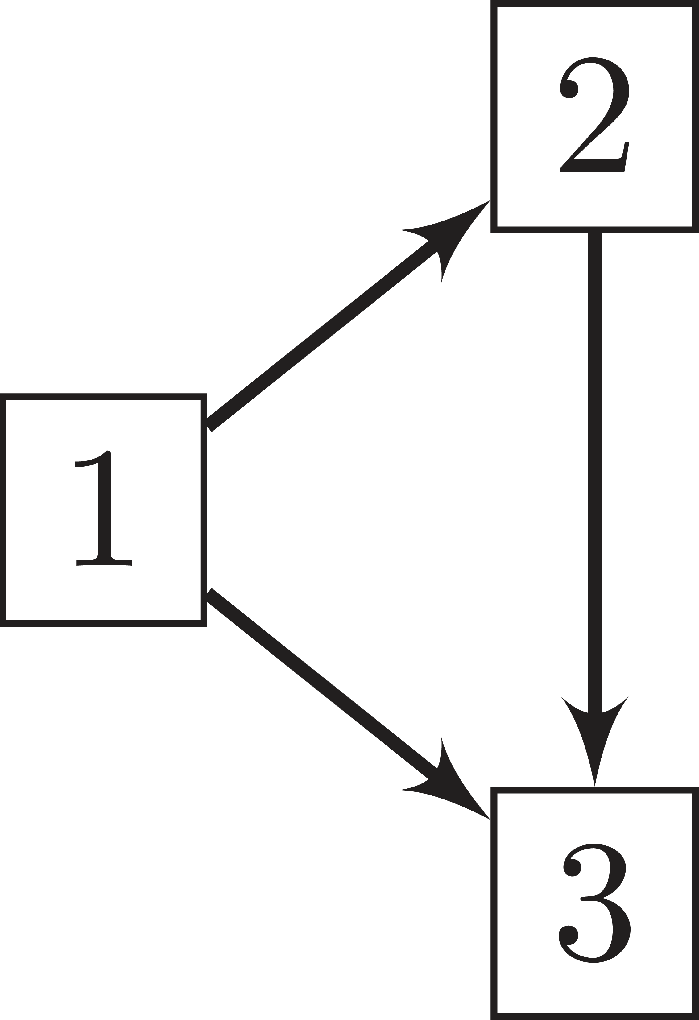
From a probabilistic framework, an illness-death model is defined as a stochastic process
The random behaviour of our illness-death model is determined by the initial distribution of the process,


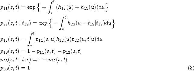
In the case of our illness-death model, transition probabilities are computed from transition intensities as indicated below.
6
In particular, note that

We propose a Bayesian spatial illness-death model for a finite spatial lattice data with a set of local neighbourhoods defined by geographic vicinity between the sites of the target region. This model includes the joint modelling of the three relevant survival times of the illness-death model associated with each site as well as a spatial structure, based on the Leroux model, 14 which connects the survival process of the different sites of the spatial domain. The notation of the Bayesian content that we will introduce from now on considers all probabilities and derived concepts to be conditional because all the parameters and hyperparameters on which they depend have probability distributions.
Sampling model
Let
Random effects
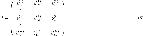

The structure of

Models for the spatial variability

We model the variance-covariance matrix

A Bayesian approach based on the integrated nested Laplace approximation (INLA)
21
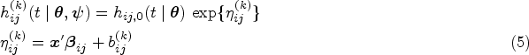
has been considered to estimate the posterior distribution of all the quantities of interest of the model. Bayesian inference combines prior knowledge of all unknown parameters and hyperparameters
As just discussed, we need to complete the Bayesian model with a prior distribution for all parameters and hyperparameters
The covariance matrix including the correlation between transitions,
A non-informative uniform prior,
Note that when working with INLA, the number of hyperparameters is an important element to take into consideration. INLA can deal with models with a large number of components in the latent field, including fixed effects for covariates and random effects. However, a small number of hyperparameters is a critical assumption required to ensure accuracy in the approximations and for computational reasons. Rue et al.
21
pointed out that a moderate amount of hyperparameters would be in the range of 6–12, while Rue et al.
32
set a maximum of 20 hyperparameters. In our analysis, we have hyperparameters from two different sources: the illness-death model and the spatial structure. As we assumed baseline risk Weibull distributions in the multistate model, we would have three
Posterior outcomes
The posterior distribution
It is worth mentioning that, by default, INLA provides approximate samples from the marginal posterior distributions and not from the joint posterior. In that sense, sampling from marginal information to infer about the outcomes of interest is not appropriate because it can produce misleading results that do not take into account the possible relationships between the components of the latent field. Fortunately, the INLA is also able to sample from the joint posterior distribution.30,35 That is what we have done in this article. In the following, we will introduce some of those outcomes discussed above and discuss their posterior estimation.
Sojourn times
Sojourn time in state
Transition probabilities depend on the parameters through the subsequent hazard functions according to (3). Therefore, their posterior distribution
Cumulative incidence functions
Cumulative incidence functions are more frequently used in competing risks environments, but they are also useful for illness-death models, specially when the illness is relevant by itself and not only as an intermediate state between the initial state and death. They can be defined equivalently to the competing scenario for survival times


Clinical settings involving the progression of non-terminal diseases, repeated events and populations with a considerable competing risk of death are the main scenarios where multi-state models can be applied. We illustrate here the application of the previous model on a study of recurrent hip fracture.
The PREV2FO cohort
We analyse the PREV2FO cohort, a population-based cohort comprising patients aged 65 years and older discharged after hospitalization for an osteoporotic hip fracture in the Valencia Region (Spain) from 1 January 2008 to 31 December 2015. 36 The Valencia Region is an autonomous community of Spain, with a population of roughly 5 million people (10% of the Spanish population). The region provides universal healthcare services through the Valencia Health System (VHS) which is an extensive network of public hospitals, primary care centres and other public resources managed autonomously by the regional government. It is divided into 24 Health Areas, each one corresponding to the administrative area of influence of a public hospital from the VHS.
Patients were followed after the index fracture until death or end of study (31 December 2016), accounting for recurrent hip fractures during the follow-up period. Figure 2 shows a diagram of this process as and illness-death model with an initial state of discharge after a first hip fracture (F), an intermediate state that accounts for discharge after a refracture (R) and the state of death (D). Transition times between states were right-censored only due to end of study or death (see Supplemental Table 1 for specific information about the number of patients that progresses between states by sex and Health Area).
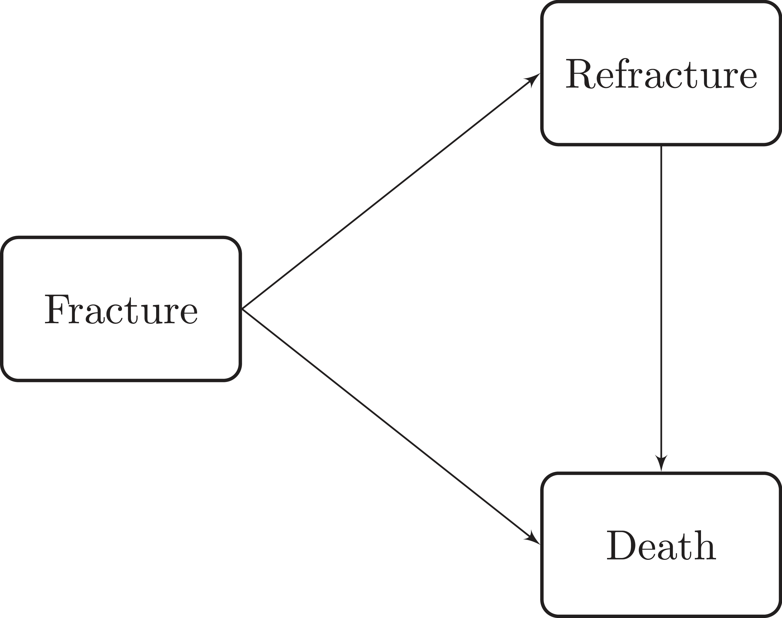
Illness-death model with an initial state of hip fracture, a recurrent hip fracture state and a death state.
From a clinical point of view, there is a possibility of more than one refracture. We have dismissed this possibility because in our study only a reduced number of the patients suffered from them. In particular, we have 2532 patients with a refracture, only 26 of them with a second refracture and only one with a third. Due to the complexity of the model and the limited information regarding more than one refracture, we decided not to include this in the model and therefore, the exact definition of our refracture state would be thus ‘having at least one refracture’. Moreover, note that our model is easily generalizable and in case we had a higher number of patients with second or third refractures, we could add the corresponding states to represent those additional transitions.
In order to define a basic patient profile we have considered sex, age at the discharge and the Health Area in which patients were hospitalised as covariates. The study involved 34491 patients discharged alive after hip fracture, 25807 (74.8
Survival times from state
We present the approximated posterior distribution sequentially, first the parameters, then the hyperparameters and finally, the random effects. Table 1 summarises the approximate posterior marginal distribution of all parameters of the model. Estimations of the shape parameters of the baseline risk functions,
Summary of the approximate posterior distribution of the parameters from an illness-death model with a multivariate-Leroux model for random effects. Transition-related parameters: shape of Weibull distribution and regression coefficients.
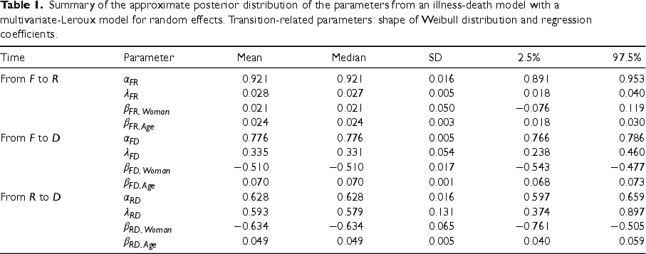
Summary of the approximate posterior distribution of the parameters from an illness-death model with a multivariate-Leroux model for random effects. Transition-related parameters: shape of Weibull distribution and regression coefficients.
Figure 3 shows the posterior expectation of the baseline hazard function associated to each of the three survival times. Note that the risks of death after recurrent hip fracture are higher than those of death without refracture. Transition intensity from fracture to refracture is notably lower than transitions to death. Note that baseline hazard functions are indeed the hazard functions for the reference values of predictors: average-aged men from a Health Area with a random effect equal to 0. Baseline functions suggest higher hazards during the first year, including the hazard of refracture, despite it cannot be appreciated graphically. It results in a sharper increase in the cumulative incidence of those events, as well as greater increases or decreases in the transition probabilities during the initial follow-up.
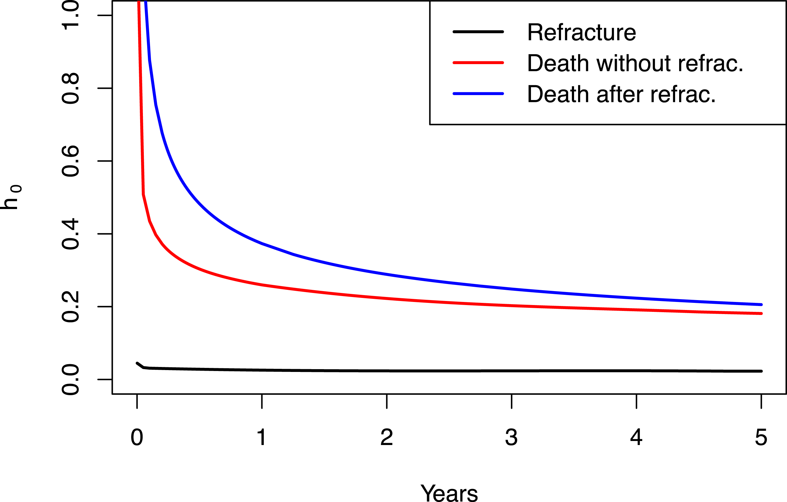
Posterior mean of the baseline hazard function for each survival transition: from
Table 2 presents a summary of the approximate posterior marginal distribution of the hyperparameters of the spatial illness-death model, all them associated with the variability between the transition survival times and within the different Health Areas in the Valencia Region. The estimation of the parameter
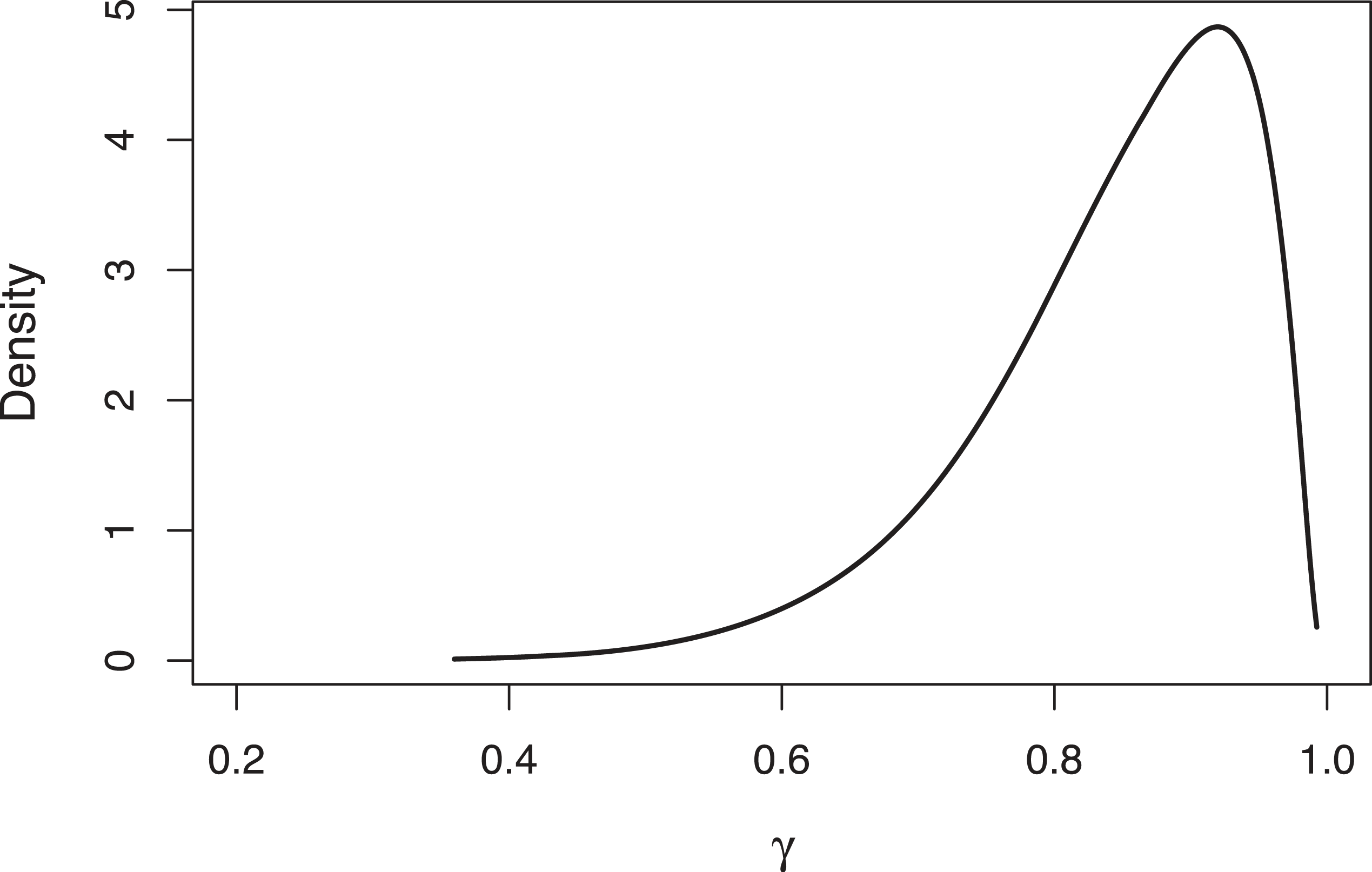
Approximated posterior distribution of the
Summary of the approximate posterior distribution of the hyperparameters from the illness-death model estimated with a multivariate-Leroux model for the spatial random effects.
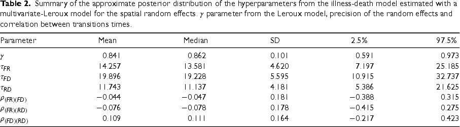
Figure 5 displays the posterior mean of the random effects associated with each transition time and Health Area of the Valencia Region. Health Areas coloured red indicate a higher risk of experiencing the event of interest compared to the overall average for all areas. Areas shaded in yellow indicate the opposite. The random effects associated with the three survival times of the illness model from the same Health Area do not always behave the same. We can observe some areas with positive random effects in the three survival times considered, but also some cases where the effects show negative relationships. There are some particular areas with a particular spatial pattern. This is the case of Requena-Utiel (the most western Health Area) and Denia (located at the cape in the east of the Valencia Region). The first shows a lower risk of recurrent hip fracture and a higher risks of death without and after refracture. The latter shows the opposite scenario, higher risk of refracture and lower mortality. Both cases illustrate a negative association between the risk of refracture and mortality, whilst a positive association between both risks of death.
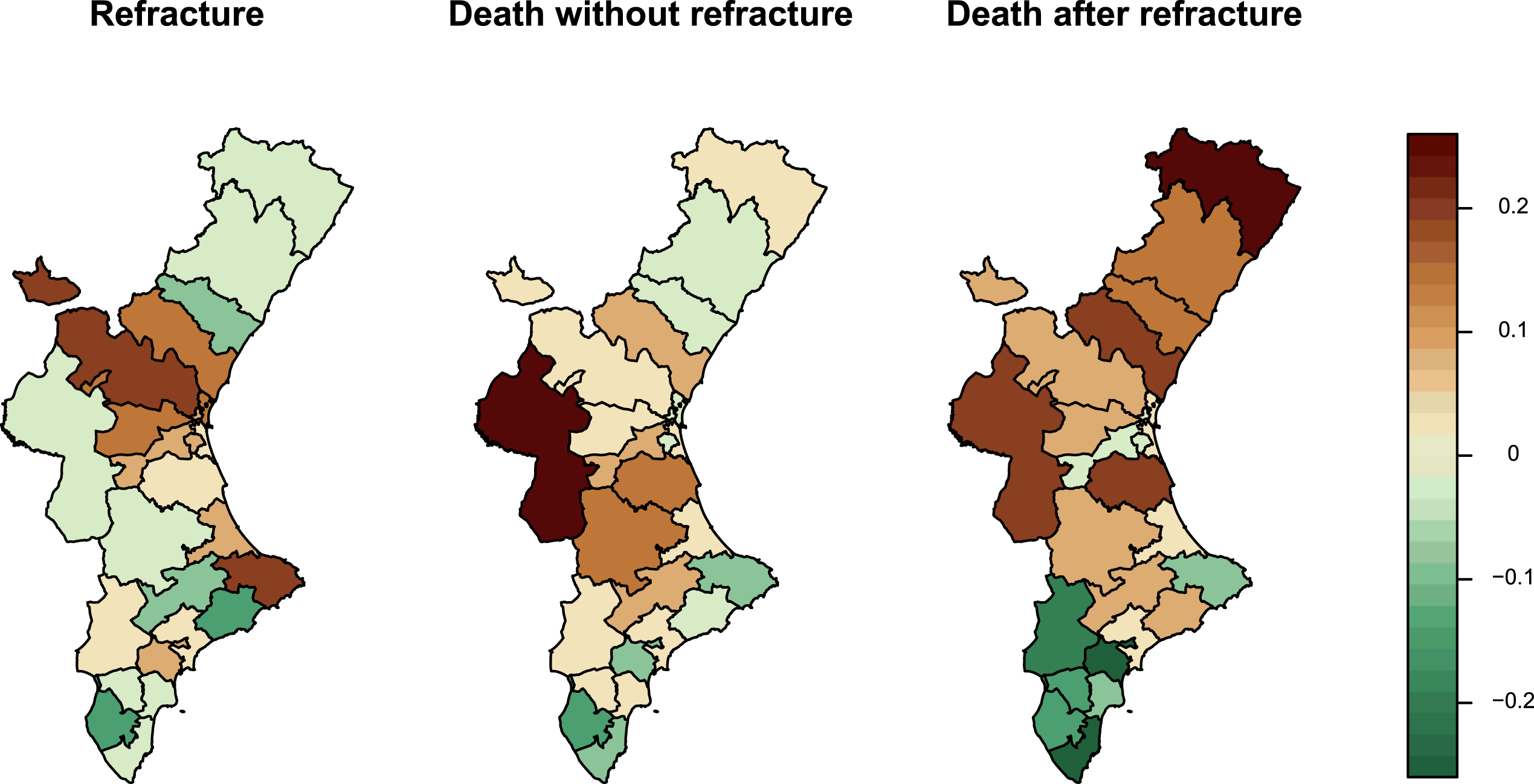
Posterior mean of the region-specific random effects by Health Area of the Valencia Region, from an illness-death model with multivariate-Leroux random effects.
The examination of the raw estimations provided by the posterior distribution
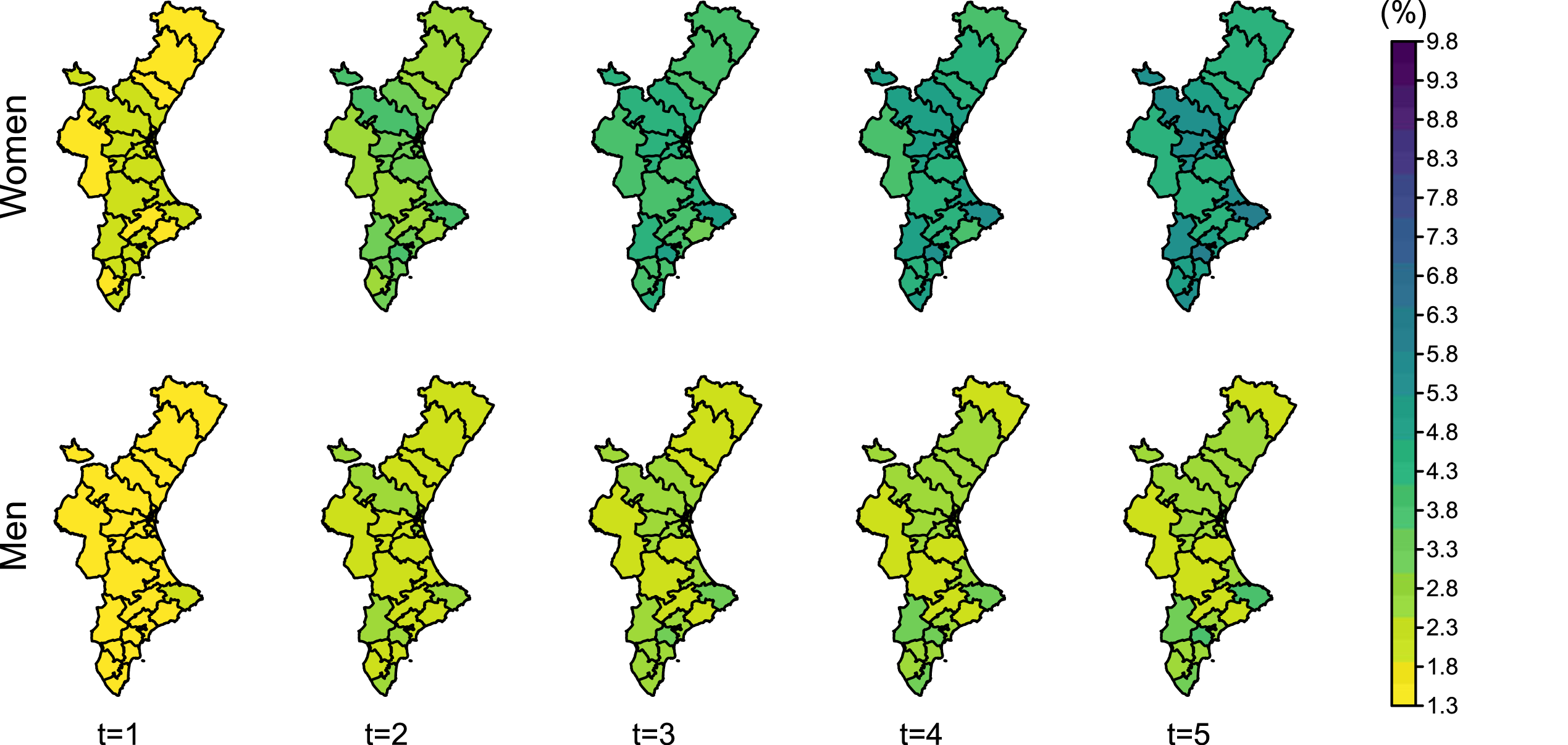
The cumulative incidence of a hip refracture at time
Posterior mean of the cumulative incidence of refracture in 80-year-old women and men at
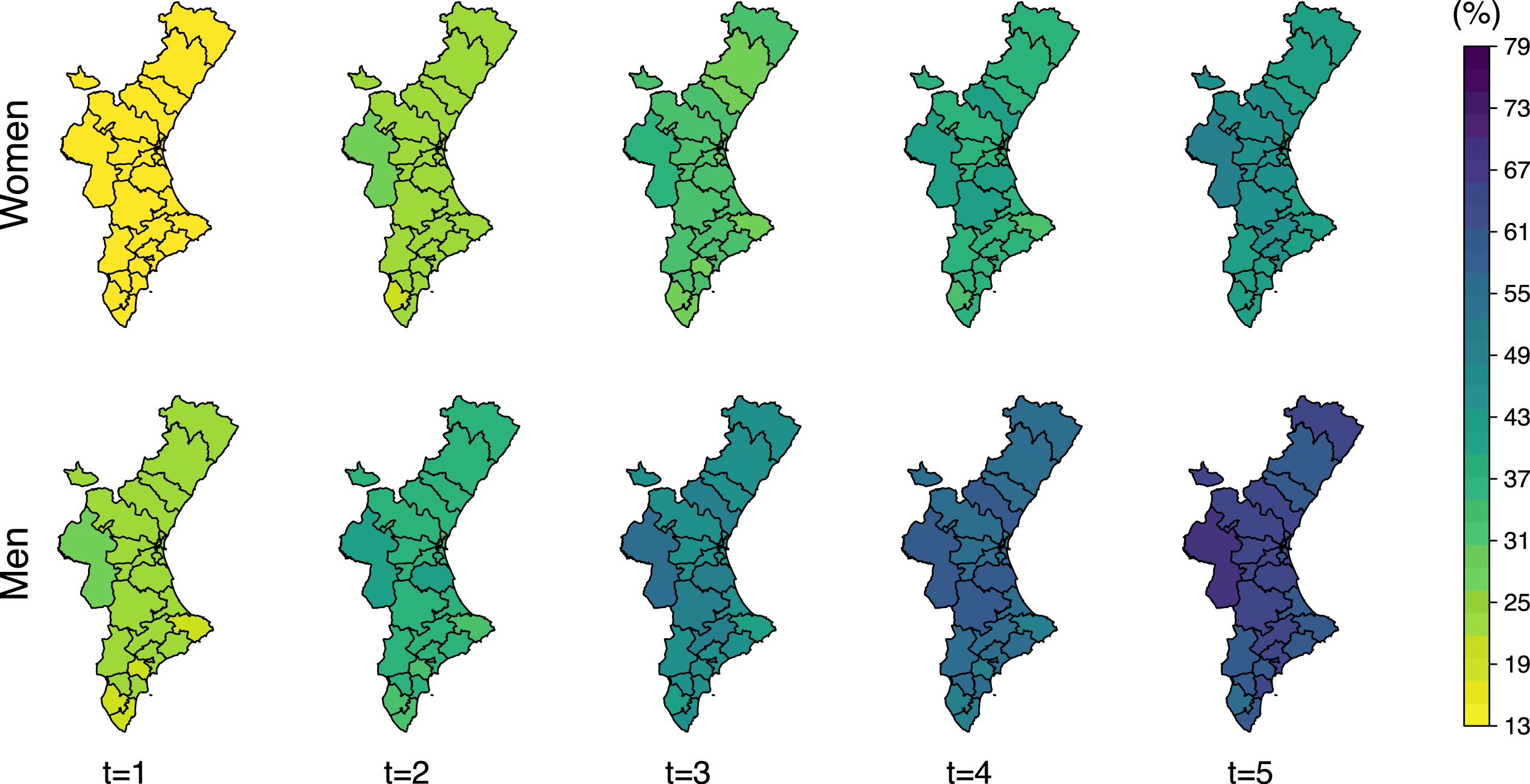
Regarding transition probabilities from fracture to refracture (Figure 7), they are also higher for women, as they are more likely to experience a refracture than men. It shows an increasing trend during 2 and 4 years from the initial fracture for men and women, respectively. After this time, the probability of being refractured and alive remains stable, as the number of patients at risk of refracture decreases and the mortality after refracture offsets the number of new refractures.
Posterior mean of the transition probability from fracture to refracture (
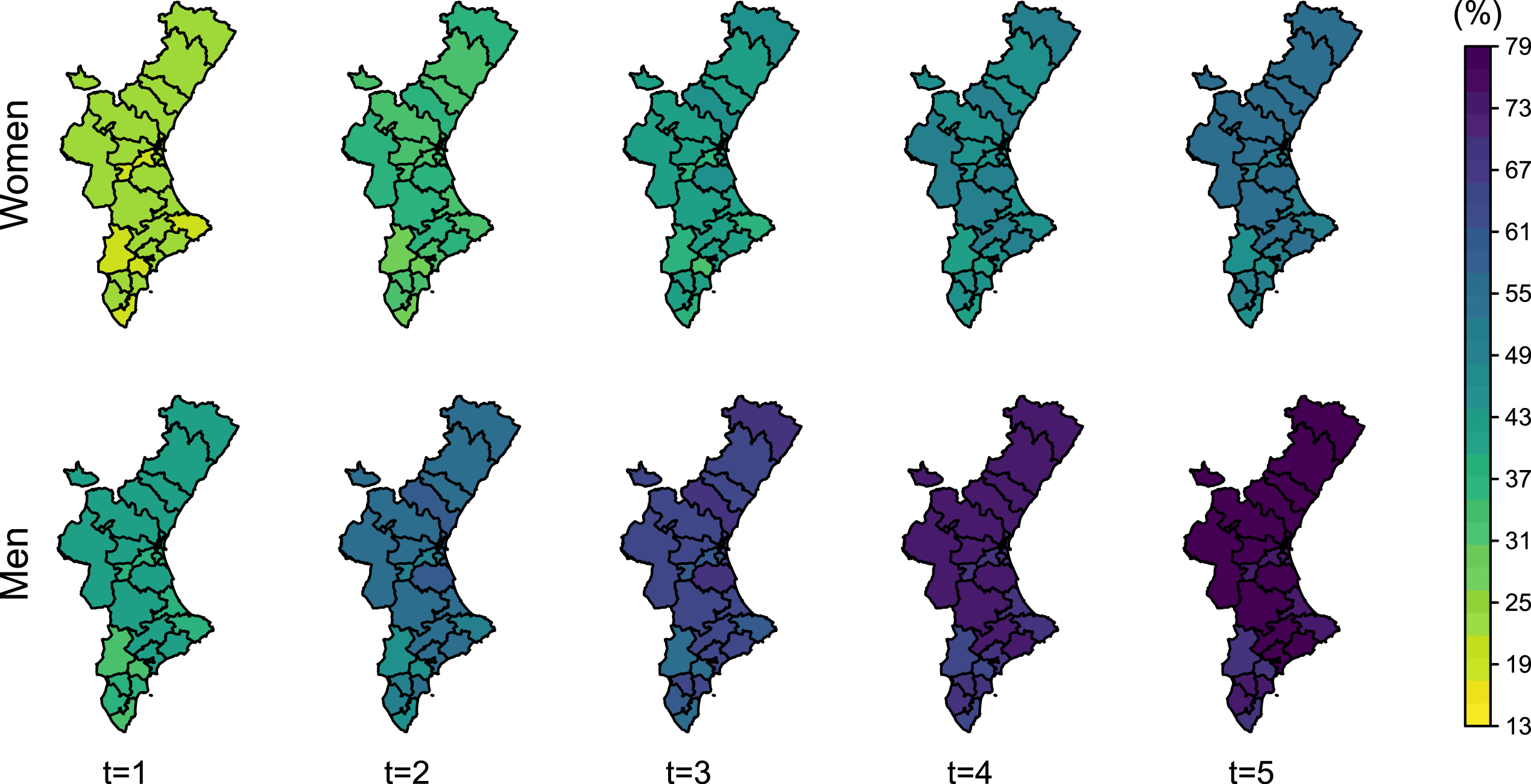
Mortality is higher in men for both, total mortality and after recurrent hip fracture, only. Women approximately reach at 4 years the same mortality than men at 2 years (Figure 8). This difference is even higher for death after a refracture. Women reach at 5 years after refracture the same mortality rates than men only 2 years after a refracture (Figure 9).
Posterior mean of the total-death probability (

Posterior mean of the probability of death after refracture (
The number of patients who die after a refracture represents a low fraction of the total mortality. Cumulative incidence of refracture indicates that less than 10% of women experience a refracture 5 years after the initial fracture (even lower in men). Thus, the spatial pattern of the total-death probability (Figure 8) is similar to that showed by the random effects on the risk of death without refracture (Figure 5).
The probability of death is higher for those patients with a recurrent hip fracture. Mortality one year after refracture is similar to that expected two years after the initial fracture. Its spatial pattern is also different with respect to that shown by total-mortality, and is identical to that shown by the respective random effects on the transition from refracture to death in Figure 5. This is due to the fact that the probability of death after refracture is the only one which depends exclusively on one transition intensity, in particular, the transition intensity from refracture to death.
The stability of posterior inferences to the specification of the different elements of the Bayesian model is an important issue in Bayesian analysis. 39 In this section, we only intend to take a brief look at the subject by analysing, in a non-exhaustive way, the sensitivity of the posterior results to the prior specification of some of the elements of the model. Obviously, these analyses do not demonstrate the robustness of the model, but they do show evidence in its favour. Likewise, and as the comparison between MCMC and INLA methods is always interesting, we have worked with a simpler model and compared the results provided by the INLA and those obtained through MCMC using JAGS.
We start focusing on the posterior inferences carried out by modifying the prior information on some hyperparameters of the spatial precision matrix. We assessed both differences in the estimations of the random effects as well as parameters and hyperparameters. Firstly, we considered the
For the comparison between MCMC methods, via JAGS, and INLA we worked with a less complex Bayesian illness-death model and reduced the space to a group of five neighbouring Health Areas. The model (see Supplemental File 1) includes Gaussian random effects with between-transition correlation, but without spatial correlation. A post-sweeping has been applied to random effects obtained from JAGS, leading to identifiable intercepts and random effects.37,38 Convergence was assessed graphically and via Gelman and Rubin’s
On the other hand, we estimated Monte Carlo Standard Errors (MCSEs)
40
for the samples of the posterior outcomes (Figures 6 to 9). Note that we first simulated values of the parameters from the joint posterior distribution with INLA, and then we obtained samples of cumulative incidences and transition probabilities. They are thus susceptible to Monte Carlo uncertainty, and we should provide the MCSE of those samples, analogously to what is done when simulating from MCMC or other methods which work with random draws. We calculated those errors for each Health Area,
Discussion
The potential and usefulness of illness-death models are highly increased after combining them with spatial information modelled by multivariate random effects associated with a set of spatial units. Differences among regions can be studied under this joint framework, in addition to the progression of individuals over time. Despite the correlation between transitions was not observed to be relevant in our real-world study, the possibility of modelling it jointly with the spatial correlation from a model based on a neighbourhood structure, such as the Leroux model, defines an extensive number of options depending on the needs of the clinical framework. Moreover, one might be interested in using more complex multi-state models with additional states and transitions. It would be analogous as the concept throughout our work regarding how random effects are included in transition intensities is quite general and, thus, it is not restricted to illness-death models.
Some extensions of our work regarding censoring and truncation 41 could be implemented without much difficulty. Patients with a hip fracture require hospitalization and, therefore, we exactly know when events occur. As a result, we had no other censoring than administrative censoring (i.e. due to end of study) or death. Note, however, that interval-censoring could arise in many survival health applications in which visits are the only way to know patients’ status. 42 A patient could reach an illness state (state 2) between two consecutive visits and thus we would only know the time interval in which the event of interest occurred. On the other hand, we have considered time since fracture as the timescale of our analysis. Patients enter the process at that time and are followed up thereafter. An alternative study of the process according to a time scale marked by the age of the patient, 43 with time zero determined by the age of 65 years, would generate left-truncated data. They would correspond to those patients who made their debut in the study, leaving the hospital already healed from the first fracture, at ages over 65 years. INLA functions for Weibull survival models can deal with right censored data, as in our case, but also interval-censored and left-truncated.
The assumption of Weibull hazard functions in the study appears to be quite consistent. Weibull hazards can only be either increasing or decreasing (as in our study). For instance, regarding recurrent hip fracture and death, decreasing hazards seem reasonable as it is known that the occurrence of those events is particularly high during the first year after a fracture. However, after some time, the risk of death might be expected to increase, showing a smooth U-shaped curve, which is not possible assuming Weibull distributions. Flexible specifications, such as those based on piecewise functions or cubic splines functions, 10 could be a good alternative to explore in future work.
The usage of the INLA is another strong point of our work. Computational time is highly reduced compared to MCMC methods, and the introduction of Gaussian random effects in the regression terms is something natural in the INLA. However, it is not a popular choice when assessing multi-state models yet, although this in the near future might change given its benefits. Multi-state modelling in INLA remains unexplored and further work regarding this issue would be of high interest.
Finally, assessing transition probabilities and cumulative incidences instead of only analysing the estimations of random effects on transition intensities provides a deeper understanding of the clinical or epidemiological problem. In fact, the risk assessment alone seldom provides predictive information regarding the prognostic of a patient given some specific characteristics. Meanwhile, trajectories expressed in terms of probabilities are dynamic and interpretable outcomes which are essential to reach an individualised care and that can be determinant to clinicians and policy makers.
Supplemental Material
sj-pdf-1-smm-10.1177_09622802231172034 - Supplemental material for A Bayesian multivariate spatial approach for illness-death survival models
Supplemental material, sj-pdf-1-smm-10.1177_09622802231172034 for A Bayesian multivariate spatial approach for illness-death survival models by Fran Llopis-Cardona, Carmen Armero and Gabriel Sanfélix-Gimeno in Statistical Methods in Medical Research
Footnotes
Acknowledgements
We thank the editor and reviewers for their thorough comments and suggestions which have substantially improved our manuscript.
Declaration of conflicting interests
The author(s) declared no potential conflicts of interest with respect to the research, authorship, and/or publication of this article.
Funding
The author(s) disclosed receipt of the following financial support for the research, authorship, and/or publication of this article: This work has been funded by Instituto de Salud Carlos III (ISCIII) through the projects [PI14/00993, PI18/01675], ‘RD16/0001/0011 – Red Temática de Servicios de Salud Orientados a Enfermedades Crónicas (REDISSEC)’, and ‘RD21/0016/0006 – Red de Investigación en Cronicidad, Atención Primaria y Promoción de la Salud (RICAPPS)’, and co-funded by the European Union. FLC was funded by Instituto de Salud Carlos III (ISCIII) [grant number FI19/00190], and co-funded by the European Union. CA was partially funded by Ministerio de Ciencia e Innovación (MCI, Spain) [grant number PID2019-106341GB-I00].
References
Supplementary Material
Please find the following supplemental material available below.
For Open Access articles published under a Creative Commons License, all supplemental material carries the same license as the article it is associated with.
For non-Open Access articles published, all supplemental material carries a non-exclusive license, and permission requests for re-use of supplemental material or any part of supplemental material shall be sent directly to the copyright owner as specified in the copyright notice associated with the article.