Copula modeling for the estimation of measures of marker classification and predictiveness performance with survival outcomes

Abstract

The discriminative and predictive power of a continuous-valued marker for survival outcomes can be summarized using the receiver operating characteristic and predictiveness curves, respectively. In this paper, fully parametric and semi-parametric copula-based constructions of the joint model of the marker and the survival time are developed for characterizing, plotting, and analyzing both curves along with other underlying performance measures. The formulations require a copula function, a parametric specification for the margin of the marker, and either a parametric distribution or a non-parametric estimator for the margin of the time to event, to respectively characterize the fully parametric and semi-parametric joint models. Estimation is carried out using maximum likelihood and a two-stage procedure for the parametric and semi-parametric models, respectively. Resampling-based methods are used for computing standard errors and confidence bounds for the various parameters, curves, and associated measures. Graphical inspection of residuals from each conditional distribution is employed as a guide for choosing a copula from a set of candidates. The performance of the estimators of various classification and predictiveness measures is assessed in simulation studies, assuming different copula and censoring scenarios. The methods are illustrated with the analysis of two markers using the familiar primary biliary cirrhosis data set.

Introduction

Marker development is a major research topic for supporting medical decision-making in the prognosis and timely treatment of progressive diseases. Consequently, the development and estimation of marker performance and decision-analytic measures are crucial topics in medical research. Important aspects of measurement include discrimination and prediction, which can be quantified by the receiver operating characteristic (ROC) and the predictiveness curves, respectively. For time-to-event data, both curves can be obtained when considering the status of a survival outcome at a certain time of the follow-up study, in order to both assess the performance of the marker and identify subjects that are at high risk of experiencing the outcome.

Previously proposed methodologies for studying time-varying performance measures have mainly addressed the estimation of a specific type of ROC curve only by employing non-parametric and semi-parametric (SP) techniques ¹ ; also, the estimation of the time-varying area under the ROC curve, which is a measure that describes the discriminatory value of the marker, has been an ongoing research focus, with existing smoothing methods proving to be cumbersome when it comes to implementation. ² Furthermore, the estimates of the ROC curve and its summaries when employing kernel smoothing methods are not transformation invariant; that is, monotone transformations to either the marker or the survival time, or both, may lead to different estimates for the ROC curve and its summaries. ³ This is exacerbated by the fact that there is no methodology that brings both curves and their summaries together under a common framework, with a partial estimation of the predictiveness curve being the best scenario when a parametric ROC model is provided. ⁴

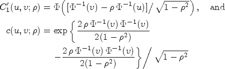
Since employing different techniques to separately estimate measures from each curve may potentially result in misleading inferences, the correct representation of the joint model of the continuous-valued marker $M$ and the survival time $T$ should both enable the characterization of both curves and lead to coherent estimates. In this paper, two copula-based approaches are proposed to characterize such joint model. The first model is an extension of the model for cross-sectional data in Escarela et al., ⁵ which is conveniently constructed by customizing and linking with a copula a parametric marginal continuous cumulative distribution function (CDF) for $M$ and a parametric marginal survival distribution function for $T$ , leading to a fully parametric (FP) formulation. Such construction is appealing since the copula that characterizes the joint behavior of monotone increasing transforms of $M$ and $T$ is exactly the same copula as for the original pair $(M,T)$ ; that is, the unique copula associated with $(M,T)$ is invariant under monotone increasing transformations of the margins, ⁶ which clearly benefits both the modeling and the inference process.

The second model represents the joint density function of the marker and the survival time by applying a latent variable transformation to the margin of the survival time in the aforementioned parametric copula model, in such a way that the transformed model allows for the marginal survival distribution of the time to event to be specified as discrete, resulting in a SP specification that is particularly useful when the parametric margin of $T$ does not appear to be adequate, or when the survival data are either discrete or subject to interval-censoring. Expressions of the ROC and predictiveness curves along with their summaries are then obtained in terms of the resulting joint models. Residual-based diagnostics are proposed to criticize the fit of the two joint models and, thus, to help in the choice of a copula. Simulation studies are carried out to assess the performance of the procedures under different copula and censoring scenarios. As an illustration, the performance of two markers for survival outcomes of the Mayo Clinic Primary Biliary Cholangitis (PBC) follow-up is studied.

Methods

Background: Marker performance measures

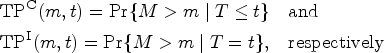
Define the dynamic false positive rate at cut-point $m$ and time $t$ as $\mathrm{FP}(m,t)=Pr\{M>m\mid T>t\}$ , and define the cumulative true positive and incident true positive rates at cut-point $m$ and time $t$ as

$$\begin{array}{rl}{\mathrm{TP}}^{\mathrm{C}}(m,t)=Pr\{M>m\mid T\le t\}& \mathrm{and}\\ {\mathrm{TP}}^{\mathrm{I}}(m,t)=Pr\{M>m\mid T=t\},& \mathrm{respectively}\end{array}$$

Two main definitions of the ROC curve have been proposed for measuring the time-dependent discriminating ability of the marker. The Cumulative/Dynamic ROC curve at time $t$ , ${\mathrm{ROC}}^{\mathrm{C}/\mathrm{D}}(q,t)$ , is defined as the plot of $\{[\mathrm{FP}(c,t),{\mathrm{TP}}^{\mathrm{C}}(c,t)];c\in \mathbb{R}\}$ , where $\mathbb{R}$ is the real line; that is

$${\mathrm{ROC}}^{\mathrm{C}/\mathrm{D}}(q,t)={\mathrm{TP}}^{\mathrm{C}}[{\mathrm{FP}}^{-1}(q,t),t]$$

(1)

where ${\mathrm{FP}}^{-1}(q,t)=\underset{c}{inf}\{c:\mathrm{FP}(q,t)\le q\}$ , for $q\in [0,1]$ . The Incident/Dynamic ROC curve at time $t$ , ${\mathrm{ROC}}^{\mathrm{I}/\mathrm{D}}(q,t)$ , is defined as the plot of $\{[\mathrm{FP}(c,t),{\mathrm{TP}}^{\mathrm{I}}(c,t)];c\in \mathbb{R}\}$ ; that is

$${\mathrm{ROC}}^{\mathrm{I}/\mathrm{D}}(q,t)={\mathrm{TP}}^{\mathrm{I}}[{\mathrm{FP}}^{-1}(q,t),t],q\in [0,1]$$

(2)

Common measures of marker discrimination effectiveness at a specific time $t$ are the areas under the ROC curve ${\mathrm{AUC}}^{\mathrm{C}/\mathrm{D}}(t)={\int }_0^1{\mathrm{ROC}}^{\mathrm{C}/\mathrm{D}}(x,t)\mathrm{d}x$ and ${\mathrm{AUC}}^{\mathrm{I}/\mathrm{D}}(t)={\int }_0^1{\mathrm{ROC}}^{\mathrm{I}/\mathrm{D}}(x,t)\mathrm{d}x$ ; here, ${\mathrm{AUC}}^{\mathrm{C}/\mathrm{D}}(t)$ is equal to the probability that the marker will assign a higher value to a randomly chosen subject who has died by time $t$ than to a randomly chosen subject who is still alive by time $t$ , whereas ${\mathrm{AUC}}^{\mathrm{I}/\mathrm{D}}(t)$ is the probability that the marker will assign a higher value to a randomly chosen subject who dies at time $t$ than to a randomly chosen subject who is still alive by time $t$ . ${\mathrm{AUC}}^{\mathrm{C}/\mathrm{D}}(t)$ is useful in a setting where discrimination accuracy of short-term survival has to be assessed, and ${\mathrm{AUC}}^{\mathrm{I}/\mathrm{D}}(t)$ is a summary that indicates time-varying performance with no need to select a specific time-frame. ¹

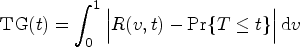
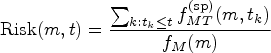
The risk function at time $t$ is defined as $\mathrm{Risk}(m,t)=Pr\{T\le t\mid M=m\}$ . If $\mathrm{Risk}(m,t)$ is monotonous increasing in $m$ at time $t$ , the time-dependent predictiveness curve is defined as

$$R(v,t)=Pr\{T\le t\mid M=F_M^{-1}(v)\}$$

(3)

where $F_M^{-1}(\cdot )$ is the quantile function corresponding to the marginal CDF of $M$ , denoted here by $F_M(\cdot )$ . The predictiveness function in equation (3) is the plot of $\{[F_M(m),\mathrm{Risk}(m,t)];m\in \mathbb{R}\}$ . For a fixed time $t$ , $R(v,t)$ displays the distribution of the predicted risk of the event occurring within time $t$ , and its inverse is the CDF of the risk function; that is, $R^{-1}(u,t)=Pr\{\mathrm{Risk}(M,t)\le u\}$ , for $u\in (0,1)$ . In clinical decision-making, pre-specified percentiles of $R^{-1}$ are used as thresholds for clustering subjects who share similar risks; for instance, if $p_U$ is the percentile for the high-risk group according to a prespecified criterion, then $1-R^{-1}(p_U,t)$ is the proportion of the population deemed to be at high risk. A summary measure of time-dependent risk prediction is the total gain, which is defined as

$$\mathrm{TG}(t)={\int }_0^1|R(v,t)-Pr\{T\le t\}|\mathrm{d}v$$

High values of total gain are obtained when the predictiveness curve is steep, which is a consequence of a useful predictive marker, reaching a maximum at time $t$ equal to $2S(t)[1-S_T(t)]$ . ⁷ An alternative summary quantification of predictiveness is the time-varying standardized total gain, which is defined as $\mathrm{STG}(t)=\mathrm{TG}(\mathrm{t})/\{2S(t)[1-S_T(t)]\}$ , and provides a time-dependent measure that allows for comparisons across different studies.

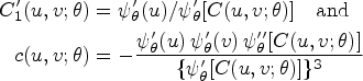
A global measure of marker usefulness can be established using a measure of concordance between the marker and the outcome such as the C-index, whose definition for survival outcomes is given by the probability that an individual who died at an earlier time $T_j$ than another individual’s $T_k$ has a larger value of the marker; that is ⁸ :

$$\text{C-index}=Pr\{M_j>M_k\mid T_j<T_k\}$$

(4)

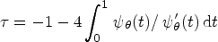
Extending the results in Liu et al., ⁹ it can be shown that the C-index can be expressed in terms of a linear combination of Kendall’s tau; namely, $\text{C-index}=(1-\tau )/2$ , where $\tau$ is Kendall’s tau, defined by

$$\begin{array}{rl}\tau & =Pr\{(M_j-M_k)(T_j-T_k)>0\}\\ & -Pr\{(M_j-M_k)(T_j-T_k)<0\}\end{array}$$

(5)

with $(M_j,T_j)$ and $(M_k,T_k)$ being independent copies of $(M,T)$ . Markers whose association with the time to event lies between that of countermonotonicity, where $\text{C-index}=1$ and $\tau =-1$ , and that of independence, where $\text{C-index}=1/2$ and $\tau =0$ , are expected to exhibit useful discriminative and predictive properties.

Copula modeling

A strategy for constructing a joint model for the continuous random vector $(M,T)$ is provided by the copula function, which is defined as a bivariate distribution function whose margins are uniform on $[0,1]$ . In the usual setting, given continuous CDF’s $F_X(x)=Pr\{X\le x\}$ and $F_Y(y)=Pr\{Y\le y\}$ of $X$ and $Y$ , respectively, Sklar’s theorem indicates that there is a unique copula $C(\cdot ,\cdot )$ such that the joint CDF of $(X,Y)$ can be defined as $F_{XY}(x,y)\equiv C[F_X(x),F_Y(y)]$ . Since some popular copulas mainly represent dependence structures whose association, as measured by Kendall’s tau, mainly cover the positive range for $F_{XY}(x,y)$ , this study instead adopts the following joint representation:

$$\begin{array}{rl}{H}_{MT}(m,t)& =Pr\{M\le m,T>t\}\\ & \equiv C[F_M(m),S_T(t)]\end{array}$$

(6)

The formulation in equation (6) is known as the semi-survival copula and the association between $M$ and $T$ is the negative of that obtained when $C$ enters the model as in the joint CDF of $(M,T)$ , ¹⁰ , thus allowing popular copula families, whose association range mainly cover the interval (0,1), to model useful discriminative and predictive markers.

Define $C_j^{\mathrm{\prime }}(u,v)=\mathrm{\partial }C(x_1,x_2)/\mathrm{\partial }{x}_j{|}_{(x_1,x_2)=(u,v)}$ , for $j=1,2$ . It can be shown that

$$\begin{array}{rl}\mathrm{FP}(m,t)& =1-H_{MT}(m,t)/S_T(t)\\ {\mathrm{TP}}^{\mathrm{C}}(m,t)& =\frac{H_{MT}(m,t)-F_M(m)-S_T(t)+1}{1-S_T(t)}\\ {\mathrm{TP}}^{\mathrm{I}}(m,t)& =1-C_2^{\mathrm{\prime }}[F_M(m),S_T(t)]\mathrm{and}\\ \mathrm{Risk}(m,t)& =1-C_1^{\mathrm{\prime }}[F_M(m),S_T(t)]\end{array}$$

Also, in the semi-survival copula setting given by equation (6), it can be shown that the corresponding Kendall’s tau can be expressed in terms of the underlying copula as Nelsen ¹¹ $\tau =1-4\int {\int }_{[0,1{]}^2}C(u,v)\mathrm{d}C(u,v)$ , which is free of marginal effects.

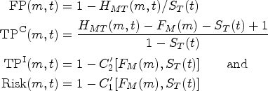
When $T$ follows a non-parametric distribution in the form of a step-wise function, with jumps at times $t_1<t_2<\cdots <t_r$ , it is possible to adopt the latent variable strategy described in de Leon and Wu ¹² in order to construct the joint model for $(M,T)$ . Assume that the random couple $(M,Y)$ is continuous, with $Y$ taking values in the positive reals, and let $T=t_k{I}_{(t_{k-1},t_k]}(Y)$ , where $I_{\mathit{A}}(x)=1$ if $x\in \mathit{A}$ and $I_{\mathit{A}}(x)=0$ otherwise, $t_0=0$ and $k=1,2,\dots r$ , then

$$\begin{array}{rl}Pr\{M\le m,T=t_k\}& =Pr\{M\le m,Y>t_{k-1}\}\\ & -Pr\{M\le m,Y>t_k\}\end{array}$$

(7)

The joint density function $f_{MT}^{(\mathrm{sp})}(m,t)$ of $(M,T)$ is obtained by differentiating equation (7) with respect to $m$ , and can be written in terms of the copula representation in equation (6) as follows:

$$\begin{array}{rl}{f}_{MT}^{(\mathrm{sp})}(m,t_k)& =f_M(m)\{C_1^{\mathrm{\prime }}[F_M(m),S_T^{(\mathrm{np})}(t_{k-1})]\\ & -C_1^{\mathrm{\prime }}[F_M(m),S_T^{(\mathrm{np})}(t_k)]\}\end{array}$$

(8)

for $k=1,2,\dots ,r$ and $m\in \mathbb{R}$ ; here, and $S_T^{(\mathrm{np})}(t)=Pr\{T>t\}$ is an ordinal discrete survival distribution, with $S_T^{(\mathrm{np})}(t)=S_T^{(\mathrm{np})}(t_k)$ for $t\in [t_k,t_{k+1})$ . The corresponding joint CDF, defined as $F_{MT}^{(\mathrm{np})}(m,t)=Pr\{M\le m,T\le t\}$ , can be computed as:

$$F_{MT}^{(\mathrm{sp})}(m,t)={\int }_{-\mathrm{\infty }}^m\sum _{k:t_k\le t}{f}_{MT}^{(\mathrm{sp})}(x,t_k)\mathrm{d}x$$

(9)

It follows that

$$\begin{array}{rl}\mathrm{FP}(m,t)& =1-\frac{F_M(m)-F_{MT}^{(\mathrm{sp})}(m,t)}{S_T^{(\mathrm{np})}(t)}\\ {\mathrm{TP}}^{\mathrm{C}}(m,t)& =1-\frac{F_{MT}^{(\mathrm{sp})}(m,t)}{1-S_T^{(\mathrm{np})}(t)}\\ {\mathrm{TP}}^{\mathrm{I}}(m,t)& =1-\frac{{\int }_{-\mathrm{\infty }}^m{f}_{MT}^{(\mathrm{sp})}(x,t)\mathrm{d}x}{S_T^{(\mathrm{np})}(t_{k-1})-S_T^{(\mathrm{np})}(t_k)}\end{array}$$

for $t\in (t_{k-1},t_k]$ , and

$$\mathrm{Risk}(m,t)=\frac{\sum _{k:t_k\le t}{f}_{MT}^{(\mathrm{sp})}(m,t_k)}{f_M(m)}$$

Inference

Estimation

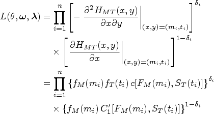
Consider the pair of marker and survival time $(M_i,T_i)$ , and let $D_i$ denote an independent right-censoring time for independent subjects $i=1,\dots ,n$ . Let $m_i$ be the observed value of $M_i$ , and let $t_i$ be the observed survival time of $min(T_i,D_i)$ and let ${\delta }_i$ be the corresponding censoring status $I(T_i=t_i)$ , where $I(\cdot )$ is an indicator function. For the FP model in equation (6), the observed likelihood function is given by

$$\begin{array}{rl}L(\theta ,\mathit{\omega },\mathit{\lambda })& =\prod _{i=1}^n{[-{\frac{{\mathrm{\partial }}^2{H}_{MT}(x,y)}{\mathrm{\partial }x\mathrm{\partial }y}|}_{(x,y)=(m_i,t_i)}]}^{{\delta }_i}\\ & \times {\left[{\frac{\mathrm{\partial }{H}_{MT}(x,y)}{\mathrm{\partial }x}|}_{(x,y)=(m_i,t_i)}\right]}^{1-{\delta }_i}\\ & =\prod _{i=1}^n{\{f_M(m_i)f_T(t_i)c[F_M(m_i),S_T(t_i)]\}}^{{\delta }_i}\\ & \times {\{f_M(m_i)C_1^{\mathrm{\prime }}[F_M(m_i),S_T(t_i)]\}}^{1-{\delta }_i}\end{array}$$

where $\theta$ is the dependence parameter of the copula function, $\mathit{\omega }$ and $\mathit{\lambda }$ are the vector of parameters of $F_M(m)$ and $S_T(t)$ , respectively, $f_M(m)=\mathrm{d}{F}_M(m)/\mathrm{d}m$ , and $c(u,v)={\mathrm{\partial }}^{2}C(u,v)/\mathrm{\partial }u\mathrm{\partial }v$ . In this study, the function nlm of the R language was employed to find the optimum of $-\log L(\theta ,\mathit{\omega },\mathit{\lambda })$ , and the corresponding Hessian. Standard errors (SEs) for the parameters can be computed as the squared root of the diagonal entries in the inverse of the observed information matrix.

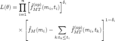
For the SP model in equation (8), a two-stage estimation procedure was adopted. The first stage involves the estimation of both margins $F_M(m)$ and $S_T^{(\mathrm{np})}(t)$ under the independence working assumption; here, maximum likelihood is used to estimate $\mathit{\omega }$ , and the Kaplan–Meier estimator is used for $S_T^{(\mathrm{np})}(t)$ . The second stage involves maximum likelihood of the dependence parameter $\theta$ with the margins held fixed from the first stage; that is, by maximizing the following likelihood function:

$$\begin{array}{rl}L(\theta )& =\prod _{i=1}^n{[{\hat{f}}_{MT}^{(\mathrm{sp})}(m_i,t_i)]}^{{\delta }_i}\\ & \times {[{\hat{f}}_M(m_i)-\sum _{k:t_k\le t_i}{\hat{f}}_{MT}^{(\mathrm{sp})}(m_i,t_k)]}^{1-{\delta }_i}\end{array}$$

where ${\hat{f}}_M(m)$ and ${\hat{f}}_{MT}^{(\mathrm{sp})}(m,t)$ are the estimators of $f_M(m)$ and $f_{MT}^{(\mathrm{sp})}(m,t)$ , respectively.

SE’s and confidence intervals (CI’s) for the various parameters and quantities can be obtained by extending the conditional bootstrap for univariate censored data in Karrison ¹³ . The resulting procedure is in fact a specialization of the non-parametric bootstrap for a copula model with censoring presented in Lawless and Yilmaz ¹⁴ , and is described as follows:

First, obtain the estimates of $\theta$ and $\mathit{\omega }$ , and of either $\mathit{\lambda }$ or $S_T^{(np)}(t)$ depending on the model specification. These are then employed to characterize the populations from which the pairs of marker and survival time are sampled.

Generate random pairs ${\mathbf{U}}^{*}=\{(u_i^{*},v_i^{*});i=1,\dots ,n\}$ from the fitted copula model $C(u,v;\hat{\theta })$ , and then obtain $m_i^{*}={\hat{F}}_M^{-1}(u_i^{*})$ and $y_i^{*}={\hat{F}}_T^{-1}(1-v_i^{*})$ , for $i=1,\dots ,n$ .

Simulate censoring times $\{d_i^{*};i=1,\dots n\}$ from an estimated censoring distribution, which can be obtained from the Kaplan–Meier estimate of $\{(t_i,1-{\delta }_i);i=1,\dots ,n\}$ , and then let $t_i^{*}=min(y_i^{*},d_i^{*})$ and ${\delta }_i^{*}=I(T_i^{*}=t_i^{*})$ .

Obtain the estimates ${\hat{\theta }}^{*}$ , ${\hat{\mathit{\omega }}}^{*}$ , ${\hat{\mathit{\lambda }}}^{*}$ for the bootstrap dataset $\{(m_i^{*},t_i^{*},{\delta }_i^{*});i=1,\dots n\}$ .

Compute the statistic of interest ${\hat{s}}^{*}=s({\hat{\theta }}^{*},{\hat{\mathit{\omega }}}^{*},{\hat{\mathit{\lambda }}}^{*})$ .

Repeat steps 2–5 $B$ number of times.

With the sequence of bootstrap estimates ${\hat{s}}^{*}$ , the corresponding standard deviation is estimated by computing the standard deviation of the estimates. Also, a $100(1-\alpha )\mathrm{\%}$ for $s$ can be estimated using the pivotal method, ¹⁵ which is computed as $(2\hat{s}-{\tilde{F}}_{{\hat{s}}^{*}}^{-1}(\alpha /2),2\hat{s}-{\tilde{F}}_{{\hat{s}}^{*}}^{-1}(1-\alpha /2))$ , where $\hat{s}$ is the point estimator of $s$ from the observed dataset, and ${\tilde{F}}_{{\hat{s}}^{*}}^{-1}(\cdot )$ is the empirical quantile function corresponding to the CDF of the bootstrap estimates ${\hat{s}}^{*}$ . In this study, the R package $\mathtt{c}\mathtt{o}\mathtt{p}\mathtt{u}\mathtt{l}\mathtt{a}$ was employed to obtain ${\mathbf{U}}^{*}$ from each copula family described below. In the illustration below, the implementation of the bootstrap procedure did not appear to be computationally demanding.

A strategy for copula selection from a given set can be performed using model diagnostics for each conditional distribution of each copula model, as both conditional distributions uniquely determine the joint model. Model criticism for the conditional distribution of $T$ given $M$ can be borrowed from the survival analysis literature because the marker $M$ is assumed to be always observed. Let ${\hat{\mathrm{\Lambda }}}_i=-\log [{\hat{S}}_{T\mid M}(t_i\mid M=m_i)]$ be the estimated conditional cumulative hazard at time $t_i$ given that $M=m_i$ , with ${\hat{S}}_{T\mid M}(t\mid M=m)$ being the estimate of $Pr\{T>t\mid M=m\}$ and computed as the estimate of $1-\mathrm{Risk}(m,t)$ . If ${\hat{S}}_{\mathrm{\Lambda }}(\mathrm{\Lambda })$ denotes the Kaplan–Meier for $\{({\hat{\mathrm{\Lambda }}}_i,{\delta }_i);i=1,\dots ,n\}$ and the conditional distribution of $T$ given $M$ is correct, then the plot of $\log [-\log {\hat{S}}_{\mathrm{\Lambda }}({\hat{\mathrm{\Lambda }}}_i)]$ vs $\log ({\hat{\mathrm{\Lambda }}}_i)$ for $i=1,\dots ,n$ , should roughly yield a straight line with slope $1$ .

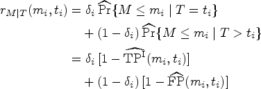
Residuals for assessing the distribution of $M$ given $T$ can be obtained by modifying Dunn and Smyth’s ¹⁶ normalized quantile residuals for a univariate continuous CDF $F_X(x)$ . If $(x_1,x_2,\dots ,x_n)$ denotes the observed random sample, such quantile residuals are defined as $r_i={\mathrm{\Phi }}^{-1}({\hat{F}}_X(x_i))$ , where ${\hat{F}}_X(x_i)$ denotes the fitted distribution function of $X$ for the $i$ -th subject. If $F_X(x)$ is correct, the residuals are independent and exactly normal, and thus usual graphic inspections, such as the quantile-quantile plot, can be employed for the assessment; in the current conditional context, however, such residuals $r_{M\mid T}(m_i,t_i)$ must be defined according to the censoring status as either the estimate of the conditional CDF of $M$ given that $T$ has been observed, or the conditional CDF of $M$ given that $T$ exceeds the censoring time; that is,

$$\begin{array}{rl}{r}_{M\mid T}(m_i,t_i)& ={\delta }_i\widehat{Pr}\{M\le m_i\mid T=t_i\}\\ & +(1-{\delta }_i)\widehat{Pr}\{M\le m_i\mid T>t_i\}\\ & ={\delta }_i[1-\widehat{{\mathrm{TP}}^{\mathrm{I}}}(m_i,t_i)]\\ & +(1-{\delta }_i)[1-\widehat{\mathrm{FP}}(m_i,t_i)]\end{array}$$

Families of copulas and margins

This study employed the four most commonly applied copula families, including the Gaussian which is defined as $C(u,v;\rho )={\mathrm{\Phi }}_2[{\mathrm{\Phi }}^{-1}(u),{\mathrm{\Phi }}^{-1}(v);\rho ]$ , where ${\mathrm{\Phi }}_2(\cdot ,\cdot ;\rho )$ is the joint CDF of the bivariate Gaussian distribution with the vector of means equal to $(0,0{)}^T$ , and the covariance matrix equal to a $2\times 2$ non-singular matrix with $1$ in each diagonal entry and the dependence parameter $\rho$ in each off-diagonal entry, $\rho \in [-1,1]$ , and ${\mathrm{\Phi }}^{-1}(\cdot )$ is the inverse of the standard normal CDF $\mathrm{\Phi }(\cdot )$ . The corresponding conditional copula and the copula density functions are ¹⁷

$$\begin{array}{rl}{C}_1^{\mathrm{\prime }}(u,v;\rho )& =\mathrm{\Phi }\left([{\mathrm{\Phi }}^{-1}(v)-\rho {\mathrm{\Phi }}^{-1}(u)]/\sqrt{1-{\rho }^2}\right),\text{and}\\ c(u,v;\rho )& =\exp \{\frac{2\rho {\mathrm{\Phi }}^{-1}(v){\mathrm{\Phi }}^{-1}(v)}{2(1-{\rho }^2)}\\ & -\frac{2\rho {\mathrm{\Phi }}^{-1}(v){\mathrm{\Phi }}^{-1}(v)}{2(1-{\rho }^2)}\}/\sqrt{1-{\rho }^2}\end{array}$$

respectively; also, it can be verified ¹⁸ that Kendall’s tau for $H(m,t)$ is given by $\tau =-(2/\pi )\arcsin (\rho )$ , implying that the range of useful markers corresponds to $\rho \in (0,1)$ . In the estimation, this study adopted an arctanh-link (Fisher’s transformation) for $\rho$ , so that $\rho$ takes values in $[-1,1]$ .

Three popular copulas belonging to the Archimedean class were also employed in this study. The Archimedean class considered here is represented as $C(u,v;\theta )={\psi }_{\theta }^{-1}[{\psi }_{\theta }(u)+{\psi }_{\theta }(v)]$ , where ${\psi }_{\theta }(\cdot )$ is a convex decreasing generating function with parameter $\theta$ that satisfy ${\psi }_{\theta }(0)=\mathrm{\infty }$ and ${\psi }_{\theta }(1)=0$ . It can be shown that the conditional copula and the copula density functions can be written in terms of the generating function and its derivatives as ¹⁹ :

$$\begin{array}{rl}{C}_1^{\mathrm{\prime }}(u,v;\theta )& ={\psi }_{\theta }^{\mathrm{\prime }}(u)/{\psi }_{\theta }^{\mathrm{\prime }}[C(u,v;\theta )]\text{and}\\ c(u,v;\theta )& =-\frac{{\psi }_{\theta }^{\mathrm{\prime }}(u){\psi }_{\theta }^{\mathrm{\prime }}(v){\psi }_{\theta }^{\mathrm{″}}[C(u,v;\theta )]}{\{{\psi }_{\theta }^{\mathrm{\prime }}[C(u,v;\theta )]{\}}^3}\end{array}$$

respectively, and that Kendall’s tau for $H(m,t)$ is given by ²⁰ :

$$\tau =-1-4{\int }_0^1{\psi }_{\theta }(t)/{\psi }_{\theta }^{\mathrm{\prime }}(t)\mathrm{d}t$$

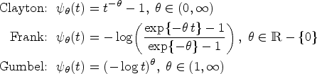
This study adopted the following Archimedean copulas, which are characterized by their generating functions:

$$\begin{array}{rl}\text{Clayton: ,}& {\psi }_{\theta }(t)=t^{-\theta }-1,\theta \in (0,\mathrm{\infty })\\ \text{Frank: ,}& {\psi }_{\theta }(t)=-\log \left(\frac{\exp \{-\theta t\}-1}{\exp \{-\theta \}-1}\right),\theta \in \mathbb{R}-\{0\}\\ \text{Gumbel: ,}& {\psi }_{\theta }(t)=(-\log t{)}^{\theta },\theta \in (1,\mathrm{\infty })\end{array}$$

In the estimation procedures described above, the dependence parameter of the Clayton and Gumbel copulas were parameterized as $\theta =\exp (\kappa )$ and $\theta =\exp (\kappa )+1$ , respectively, so that the parameter space is bounded accordingly while the parameter $\kappa$ takes values in the real line.

Since biomarkers are often skewed, ²¹ this study adopted the skewed-normal distribution for the marginal distribution of $M$ , whose probability density function (PDF) is characterized by ²² :

$$f_M(m;\mathit{\omega })=\frac{2}{{\omega }_2}\varphi \left(\frac{m-{\omega }_1}{{\omega }_2}\right)\mathrm{\Phi }\left[{\omega }_3\left(\frac{m-{\omega }_1}{{\omega }_2}\right)\right]$$

(10)

where $m\in \mathbb{R}$ , $\mathit{\omega }=({\omega }_1,{\omega }_2,{\omega }_3)$ , with ${\omega }_1\in (-\mathrm{\infty },\mathrm{\infty })$ , ${\omega }_2\in (0,\mathrm{\infty })$ and ${\omega }_3\in (-\mathrm{\infty },\mathrm{\infty })$ being the location, scale and shape parameters, respectively, and $\varphi (\cdot )$ denotes the standard normal PDF. For the parametric model, it was assumed that the marginal distribution of the survival time is Weibull, with the corresponding CDF given by:

$$F_T(t;{\lambda }_1,{\lambda }_2)=1-\exp \{-{\left(\frac{t}{\lambda {}_2}\right)}^{{\lambda }_1}\}$$

(11)

where $t\in (0,\mathrm{\infty })$ , and ${\lambda }_1\in (0,\mathrm{\infty })$ and ${\lambda }_2\in (0,\mathrm{\infty })$ are the shape and scale parameters, respectively. In the estimation process, this study employed a log-link for the parameters whose parameter-space is $(0,\mathrm{\infty })$ .

Simulation studies

To evaluate and investigate the performance of the approaches developed here, datasets under the Frank and Gumbel copula models with an assumed association corresponding to $\tau =-0.5$ , and two censoring scenarios were generated and then fitted using the FP and SP models. $F_M(m)$ was taken as the skewed-normal distribution characterized in equation (10), with ${\omega }_1=0$ , ${\omega }_2=1$ and ${\omega }_3=2$ , and $F_T(t)$ was taken as the Weibull represented in equation (11), with ${\lambda }_1=1.5$ and ${\lambda }_2=1$ . The censoring times were generated from a uniform distribution over $[0,b]$ , where $b$ was determined according to a predetermined proportion of censored times $Pr\{T>D\}$ . Under the assumed families of distributions for $D$ and $T$ , it can be shown that if $D$ and $T$ are independent

$$Pr\{T>D\}=\frac{{\lambda }_2}{b{\lambda }_1}\{{\mathrm{\Gamma }}^{(\mathrm{upper})}[\frac{1}{{\lambda }_1},{\left(\frac{b}{{\lambda }_2}\right)}^{{\lambda }_1}]-\mathrm{\Gamma }\left(\frac{1}{{\lambda }_1}\right)\}$$

where ${\mathrm{\Gamma }}^{(\mathrm{upper})}(\cdot ,\cdot )$ is the upper incomplete gamma function and $\mathrm{\Gamma }(\cdot )$ is the gamma function; thus, for the $40\mathrm{\%}$ and $60\mathrm{\%}$ of censored times considered in the simulations below, $b=2.2189$ and $b=1.3207$ , respectively.

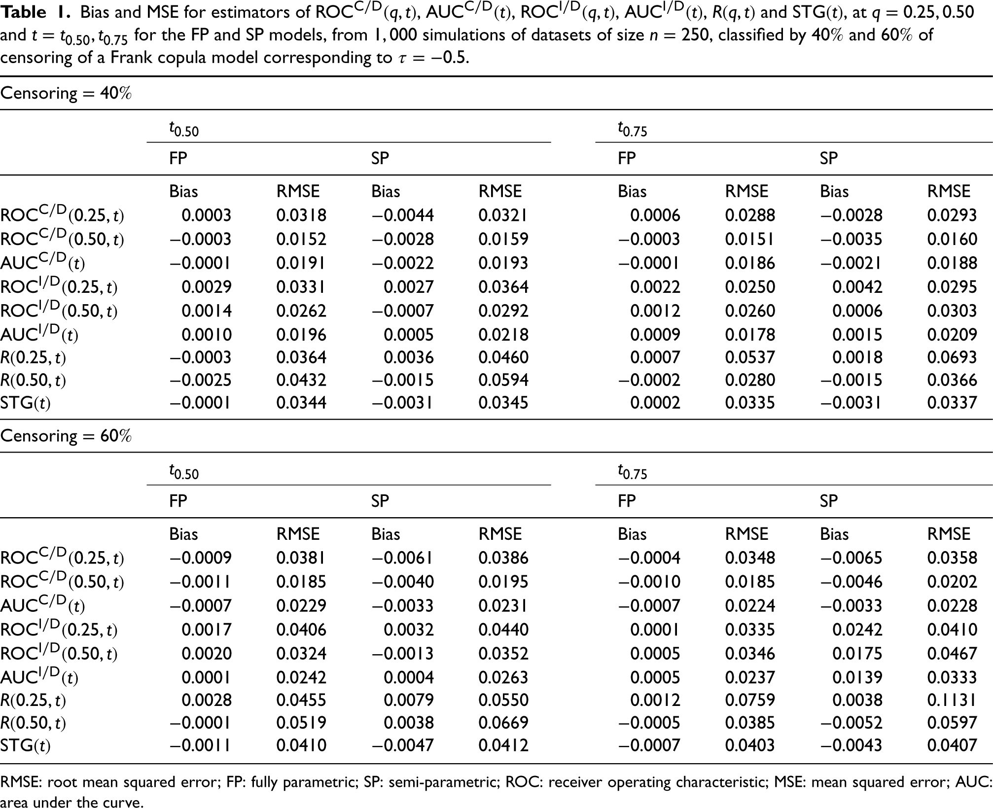
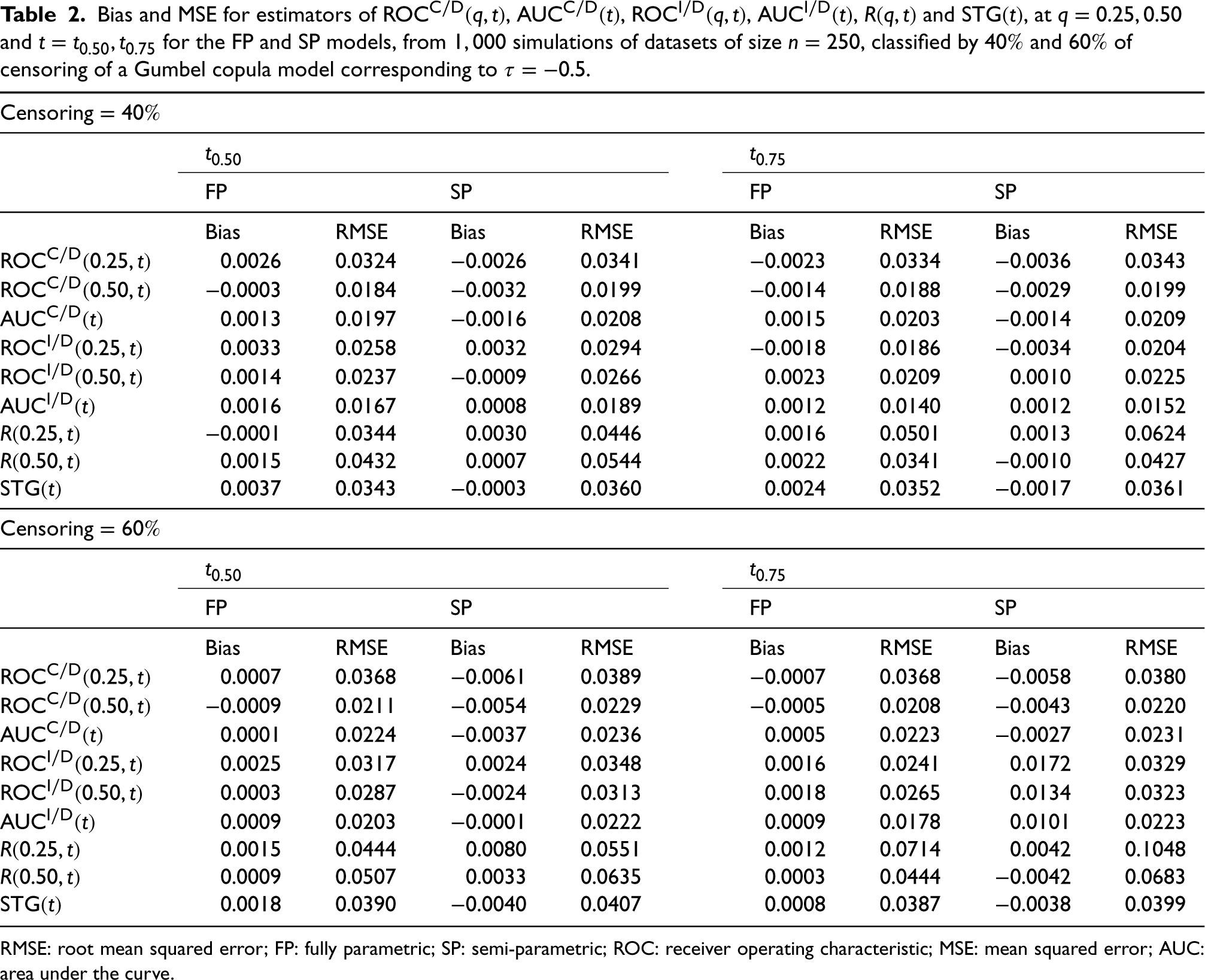
In this study, 1000 datasets of independent vectors $\{(u_i,v_i);i=1,\dots ,250\}$ from the Gumbel copula with uniform margins on $[0,1]$ were generated. The marker and actual survival time were computed as $m_i={\hat{F}}_M^{-1}(u_i)$ and $y_i={\hat{F}}_T^{-1}(1-v_i)$ , respectively. For each dataset, censoring times $\{d_i;i=1,\dots n\}$ from a uniform distribution over $[0,b]$ were generated, and the survival time and the corresponding censoring indicator were computed as $t_i=min(y_i,d_i)$ and ${\delta }_i=I(T_i=t_i)$ , respectively. The FP and SP models were then fitted to the resulting dataset, given by $\{(m_i,t_i,{\delta }_i);i=1,\dots n\}$ ; here, the parametric families were correctly specified in the corresponding components to construct both models. Results of bias and root mean squared error (RMSE) of the estimators from the FP and SP models for ${\mathrm{ROC}}^{\mathrm{C}/\mathrm{D}}(q,t)$ , ${\mathrm{AUC}}^{\mathrm{C}/\mathrm{D}}(t)$ , ${\mathrm{ROC}}^{\mathrm{I}/\mathrm{D}}(q,t)$ , ${\mathrm{AUC}}^{\mathrm{I}/\mathrm{D}}(t)$ , $R(q,t)$ and $\mathrm{STG}(t)$ , for $q=0.25$ , and $q=0.50$ at the median $t_{0.50}$ and third quartile $t_{0.75}$ of $T$ , classified by $40\mathrm{\%}$ and $60\mathrm{\%}$ of censored times, for the Frank and Gumbel copula models are shown, respectively, in Tables (1) and (2).

Table 1.

Bias and MSE for estimators of ${\mathrm{ROC}}^{\mathrm{C}/\mathrm{D}}(q,t)$ , ${\mathrm{AUC}}^{\mathrm{C}/\mathrm{D}}(t)$ , ${\mathrm{ROC}}^{\mathrm{I}/\mathrm{D}}(q,t)$ , ${\mathrm{AUC}}^{\mathrm{I}/\mathrm{D}}(t)$ , $R(q,t)$ and $\mathrm{STG}(t)$ , at $q=0.25,0.50$ and $t=t_{0.50},t_{0.75}$ for the FP and SP models, from $1,000$ simulations of datasets of size $n=250$ , classified by $40\mathrm{\%}$ and $60\mathrm{\%}$ of censoring of a Frank copula model corresponding to $\tau =-0.5$ .

$\mathrm{Censoring}=40\mathrm{\%}$
	$t_{0.50}$		$t_{0.75}$
	FP	SP		FP	SP
	Bias	RMSE	Bias	RMSE		Bias	RMSE	Bias	RMSE
${\mathrm{ROC}}^{\mathrm{C}/\mathrm{D}}(0.25,t)$	$0.0003$	$0.0318$	− $0.0044$	$0.0321$		$0.0006$	$0.0288$	− $0.0028$	$0.0293$
${\mathrm{ROC}}^{\mathrm{C}/\mathrm{D}}(0.50,t)$	− $0.0003$	$0.0152$	− $0.0028$	$0.0159$		− $0.0003$	$0.0151$	− $0.0035$	$0.0160$
${\mathrm{AUC}}^{\mathrm{C}/\mathrm{D}}(t)$	− $0.0001$	$0.0191$	− $0.0022$	$0.0193$		− $0.0001$	$0.0186$	− $0.0021$	$0.0188$
${\mathrm{ROC}}^{\mathrm{I}/\mathrm{D}}(0.25,t)$	$0.0029$	$0.0331$	$0.0027$	$0.0364$		$0.0022$	$0.0250$	$0.0042$	$0.0295$
${\mathrm{ROC}}^{\mathrm{I}/\mathrm{D}}(0.50,t)$	$0.0014$	$0.0262$	− $0.0007$	$0.0292$		$0.0012$	$0.0260$	$0.0006$	$0.0303$
${\mathrm{AUC}}^{\mathrm{I}/\mathrm{D}}(t)$	$0.0010$	$0.0196$	$0.0005$	$0.0218$		$0.0009$	$0.0178$	$0.0015$	$0.0209$
$R(0.25,t)$	− $0.0003$	$0.0364$	$0.0036$	$0.0460$		$0.0007$	$0.0537$	$0.0018$	$0.0693$
$R(0.50,t)$	− $0.0025$	$0.0432$	− $0.0015$	$0.0594$		− $0.0002$	$0.0280$	− $0.0015$	$0.0366$
$\mathrm{STG}(t)$	− $0.0001$	$0.0344$	− $0.0031$	$0.0345$		$0.0002$	$0.0335$	− $0.0031$	$0.0337$
$\mathrm{Censoring}=60\mathrm{\%}$
	$t_{0.50}$		$t_{0.75}$
	FP	SP		FP	SP
	Bias	RMSE	Bias	RMSE		Bias	RMSE	Bias	RMSE
${\mathrm{ROC}}^{\mathrm{C}/\mathrm{D}}(0.25,t)$	− $0.0009$	$0.0381$	− $0.0061$	$0.0386$		− $0.0004$	$0.0348$	− $0.0065$	$0.0358$
${\mathrm{ROC}}^{\mathrm{C}/\mathrm{D}}(0.50,t)$	− $0.0011$	$0.0185$	− $0.0040$	$0.0195$		− $0.0010$	$0.0185$	− $0.0046$	$0.0202$
${\mathrm{AUC}}^{\mathrm{C}/\mathrm{D}}(t)$	− $0.0007$	$0.0229$	− $0.0033$	$0.0231$		− $0.0007$	$0.0224$	− $0.0033$	$0.0228$
${\mathrm{ROC}}^{\mathrm{I}/\mathrm{D}}(0.25,t)$	$0.0017$	$0.0406$	$0.0032$	$0.0440$		$0.0001$	$0.0335$	$0.0242$	$0.0410$
${\mathrm{ROC}}^{\mathrm{I}/\mathrm{D}}(0.50,t)$	$0.0020$	$0.0324$	− $0.0013$	$0.0352$		$0.0005$	$0.0346$	$0.0175$	$0.0467$
${\mathrm{AUC}}^{\mathrm{I}/\mathrm{D}}(t)$	$0.0001$	$0.0242$	$0.0004$	$0.0263$		$0.0005$	$0.0237$	$0.0139$	$0.0333$
$R(0.25,t)$	$0.0028$	$0.0455$	$0.0079$	$0.0550$		$0.0012$	$0.0759$	$0.0038$	$0.1131$
$R(0.50,t)$	− $0.0001$	$0.0519$	$0.0038$	$0.0669$		− $0.0005$	$0.0385$	− $0.0052$	$0.0597$
$\mathrm{STG}(t)$	− $0.0011$	$0.0410$	− $0.0047$	$0.0412$		− $0.0007$	$0.0403$	− $0.0043$	$0.0407$

RMSE: root mean squared error; FP: fully parametric; SP: semi-parametric; ROC: receiver operating characteristic; MSE: mean squared error; AUC: area under the curve.

Table 2.

Bias and MSE for estimators of ${\mathrm{ROC}}^{\mathrm{C}/\mathrm{D}}(q,t)$ , ${\mathrm{AUC}}^{\mathrm{C}/\mathrm{D}}(t)$ , ${\mathrm{ROC}}^{\mathrm{I}/\mathrm{D}}(q,t)$ , ${\mathrm{AUC}}^{\mathrm{I}/\mathrm{D}}(t)$ , $R(q,t)$ and $\mathrm{STG}(t)$ , at $q=0.25,0.50$ and $t=t_{0.50},t_{0.75}$ for the FP and SP models, from $1,000$ simulations of datasets of size $n=250$ , classified by $40\mathrm{\%}$ and $60\mathrm{\%}$ of censoring of a Gumbel copula model corresponding to $\tau =-0.5$ .

$\mathrm{Censoring}=40\mathrm{\%}$
	$t_{0.50}$		$t_{0.75}$
	FP	SP		FP	SP
	Bias	RMSE	Bias	RMSE		Bias	RMSE	Bias	RMSE
${\mathrm{ROC}}^{\mathrm{C}/\mathrm{D}}(0.25,t)$	$0.0026$	$0.0324$	− $0.0026$	$0.0341$		− $0.0023$	$0.0334$	− $0.0036$	$0.0343$
${\mathrm{ROC}}^{\mathrm{C}/\mathrm{D}}(0.50,t)$	− $0.0003$	$0.0184$	− $0.0032$	$0.0199$		− $0.0014$	$0.0188$	− $0.0029$	$0.0199$
${\mathrm{AUC}}^{\mathrm{C}/\mathrm{D}}(t)$	$0.0013$	$0.0197$	− $0.0016$	$0.0208$		$0.0015$	$0.0203$	− $0.0014$	$0.0209$
${\mathrm{ROC}}^{\mathrm{I}/\mathrm{D}}(0.25,t)$	$0.0033$	$0.0258$	$0.0032$	$0.0294$		− $0.0018$	$0.0186$	− $0.0034$	$0.0204$
${\mathrm{ROC}}^{\mathrm{I}/\mathrm{D}}(0.50,t)$	$0.0014$	$0.0237$	− $0.0009$	$0.0266$		$0.0023$	$0.0209$	$0.0010$	$0.0225$
${\mathrm{AUC}}^{\mathrm{I}/\mathrm{D}}(t)$	$0.0016$	$0.0167$	$0.0008$	$0.0189$		$0.0012$	$0.0140$	$0.0012$	$0.0152$
$R(0.25,t)$	− $0.0001$	$0.0344$	$0.0030$	$0.0446$		$0.0016$	$0.0501$	$0.0013$	$0.0624$
$R(0.50,t)$	$0.0015$	$0.0432$	$0.0007$	$0.0544$		$0.0022$	$0.0341$	− $0.0010$	$0.0427$
$\mathrm{STG}(t)$	$0.0037$	$0.0343$	− $0.0003$	$0.0360$		$0.0024$	$0.0352$	− $0.0017$	$0.0361$
$\mathrm{Censoring}=60\mathrm{\%}$
	$t_{0.50}$		$t_{0.75}$
	FP	SP		FP	SP
	Bias	RMSE	Bias	RMSE		Bias	RMSE	Bias	RMSE
${\mathrm{ROC}}^{\mathrm{C}/\mathrm{D}}(0.25,t)$	$0.0007$	$0.0368$	− $0.0061$	$0.0389$		− $0.0007$	$0.0368$	− $0.0058$	$0.0380$
${\mathrm{ROC}}^{\mathrm{C}/\mathrm{D}}(0.50,t)$	− $0.0009$	$0.0211$	− $0.0054$	$0.0229$		− $0.0005$	$0.0208$	− $0.0043$	$0.0220$
${\mathrm{AUC}}^{\mathrm{C}/\mathrm{D}}(t)$	$0.0001$	$0.0224$	− $0.0037$	$0.0236$		$0.0005$	$0.0223$	− $0.0027$	$0.0231$
${\mathrm{ROC}}^{\mathrm{I}/\mathrm{D}}(0.25,t)$	$0.0025$	$0.0317$	$0.0024$	$0.0348$		$0.0016$	$0.0241$	$0.0172$	$0.0329$
${\mathrm{ROC}}^{\mathrm{I}/\mathrm{D}}(0.50,t)$	$0.0003$	$0.0287$	− $0.0024$	$0.0313$		$0.0018$	$0.0265$	$0.0134$	$0.0323$
${\mathrm{AUC}}^{\mathrm{I}/\mathrm{D}}(t)$	$0.0009$	$0.0203$	− $0.0001$	$0.0222$		$0.0009$	$0.0178$	$0.0101$	$0.0223$
$R(0.25,t)$	$0.0015$	$0.0444$	$0.0080$	$0.0551$		$0.0012$	$0.0714$	$0.0042$	$0.1048$
$R(0.50,t)$	$0.0009$	$0.0507$	$0.0033$	$0.0635$		$0.0003$	$0.0444$	− $0.0042$	$0.0683$
$\mathrm{STG}(t)$	$0.0018$	$0.0390$	− $0.0040$	$0.0407$		$0.0008$	$0.0387$	− $0.0038$	$0.0399$

RMSE: root mean squared error; FP: fully parametric; SP: semi-parametric; ROC: receiver operating characteristic; MSE: mean squared error; AUC: area under the curve.

Both Tables show similar results, with the FP model tending to exhibit smaller biases and RMSE’s than the estimators of the SP model, more notably when censoring is $60\mathrm{\%}$ . Discrepancies between the two estimators do not appear to be relevant for all scenarios, and there are no noticeable differences or trends when varying $q$ and $t$ . In general, all estimators perform well, showing relatively small biases and RMSE’s.

Illustration: Application to the PBC dataset

The methods presented in this study are illustrated using data from the Mayo Clinic trial in PBC conducted between 1974 and 1984, which is available in the survival package of the R program. PBC is an autoimmune disease in which the bile ducts in the liver are slowly destroyed, leading to irreversible scarring of liver tissue (cirrhosis), and eventually liver decompensation and, consequently, premature death. ²³ Patients with PBC who are at high risk of death can potentially benefit from a liver transplant, the only curative treatment for PBC ²⁴ ; therefore, identifying such high-risk group with a marker is crucial for medical decision making.

The dataset considered here consisted of a cohort of 312 patients with PBC. There were 125 (40%) deaths and 19 liver transplant recipients during the follow-up. The main goal of the study was to assess the time-varying discriminative and predictive power of a marker in mortality outcomes after registration, and thus the time to transplantation was taken as a censored time. Similar to the illustration in Bansal and Heagerty, ²⁵ this study analyzed the performance of the following two markers, which were computed as the linear predictor obtained from the usual Cox regression model: (a) 4-cov, from the model that includes orthogonal polynomials of degree 1 of albumin and age, natural logarithm of prothobin time and edema status (two levels: Edema despite diuretic therapy and otherwise); and (b) mayo, from adding the natural logarithm of bilirubin to the set of covariates in 4-cov, thus emulating the Mayo marker. ²⁶

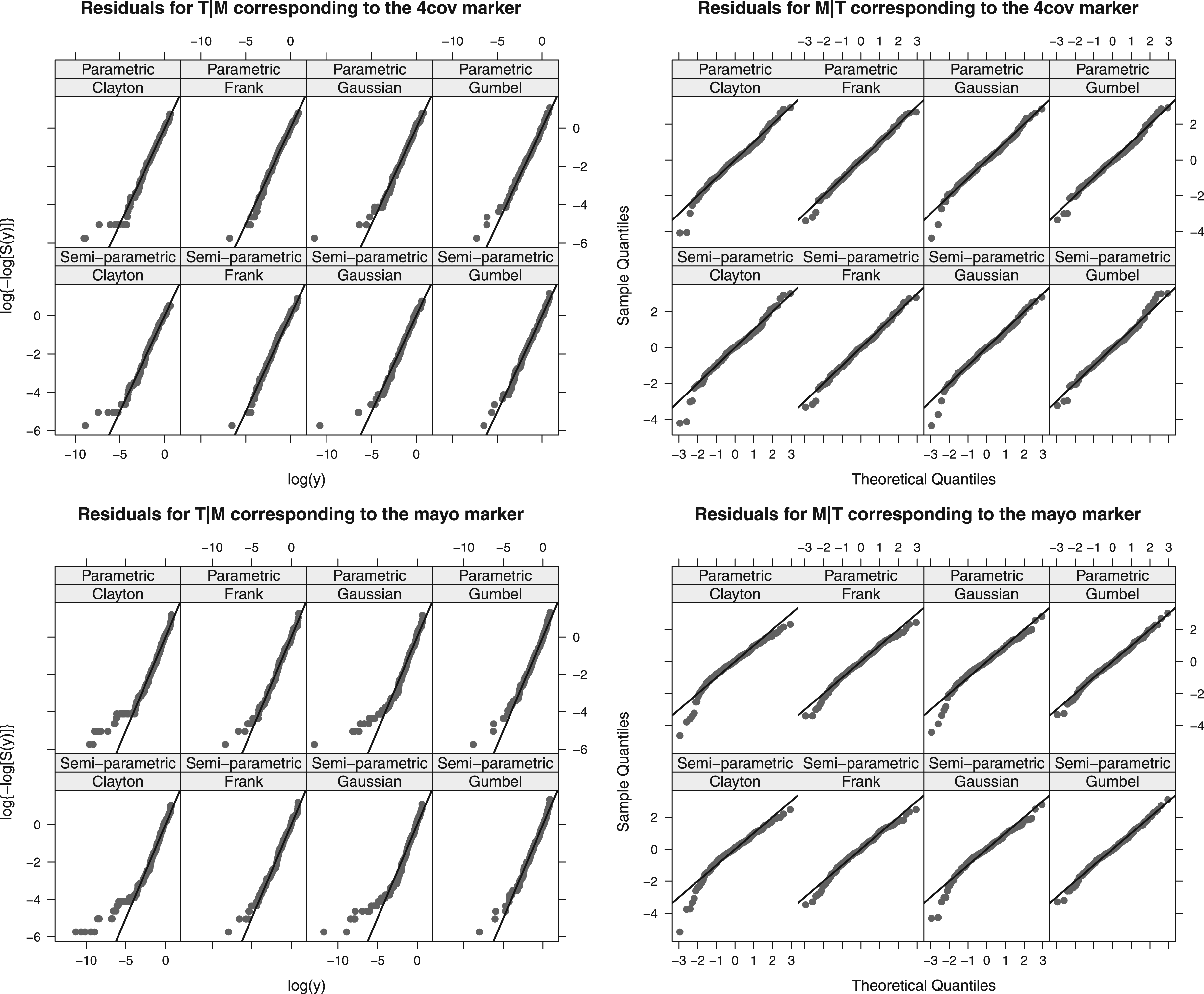
Figure 1 displays conditional residual plots for $T$ given $M$ and $M$ given $T$ of FP and SP models constructed with the Clayton, Frank, Gaussian and Gumbel copulas. The Clayton and Gaussian copulas yield the worst fits, whereas the Frank and Gumbel copulas appear to give reasonable fits to the 4-cov and mayo markers, respectively. The plots show negligible discrepancies when comparing the residuals of the FP and SP models for each copula and marker. Accordingly, this study adopted the Frank and Gumbel copulas for the 4-cov and mayo markers, respectively, in both the FP and SP models.

Figure 1.

Conditional residual plots from the fully parametric and semi-parametric model fits to the markers 4-cov and mayo using the Clayton, Frank, Gaussian and Gumbel copulas.

For the FP Frank copula model of 4-cov, it was found that the parameter $\log {\lambda }_1$ of the Weibull distribution was non-significant ( $p\text{-value}=0.55$ ), and then it was set to $0$ in order to obtain the best-fitting model; that is, an exponential distribution was used for the margin of $T$ . The maximum likelihood estimators (MLE’s) of the resulting model were: $\hat{\theta }=5.498$ (SE $0.560$ ), ${\hat{\omega }}_1=8.841$ (SE $0.490$ ), ${\widehat{\log \omega }}_2=0.490$ (SE $0.050$ ), ${\hat{\omega }}_3=4.503$ (SE $0.825$ ) and ${\widehat{\log \lambda }}_2=8.398$ (SE $0.081$ ); here, the corresponding Kendall’s tau was estimated as $\hat{\tau }=-0.487$ , with its 95% bootstrap CI computed as $(-0.535,-0.421)$ . The two-stage estimates of the SP Frank copula model for 4-cov were: $\hat{\theta }=5.061$ (SE $0.544$ ), ${\hat{\omega }}_1=8.825$ (SE $0.067$ ), ${\widehat{\log \omega }}_2=0.462$ (SE $0.051$ ) and ${\hat{\omega }}_3=4.561$ (SE $1.101$ ), with $\hat{\tau }=-0.420$ and its 95% bootstrap CI computed as $(-0.519,-0.389)$ .

For the FP Gumbel model of mayo, the parameter $\kappa$ that is linked to the dependence parameter as $\theta =\exp (\kappa )+1$ turned out not to be significant ( $p\text{-value}=0.69$ ), and then it was set to $0$ , and therefore $\theta$ was set to $2$ , which corresponds to $\tau =-0.5$ . The resulting parsimonious model yielded the following MLE’s: ${\hat{\omega }}_1=5.988$ (SE $0.077$ ), ${\widehat{\log \omega }}_2=0.842$ (SE $0.040$ ), ${\hat{\omega }}_3=6.301$ (SE $1.289$ ), ${\widehat{\log \lambda }}_1=0.136$ (SE $0.063$ ) and ${\widehat{\log \lambda }}_2=8.422$ (SE $0.082$ ). The two-stage estimation for the SP Gumbel copula model of mayo yielded $\hat{\theta }=2.022$ , with the corresponding 95% bootstrap CI computed as $(1.802,2.350)$ ; consequently, $\theta$ was set to $2$ as well, obtaining then the following estimates: ${\hat{\omega }}_1=5.975$ (SE $0.083$ ), ${\widehat{\log \omega }}_2=0.841$ (SE $0.049$ ) and ${\hat{\omega }}_3=6.595$ (SE $2.235$ ).

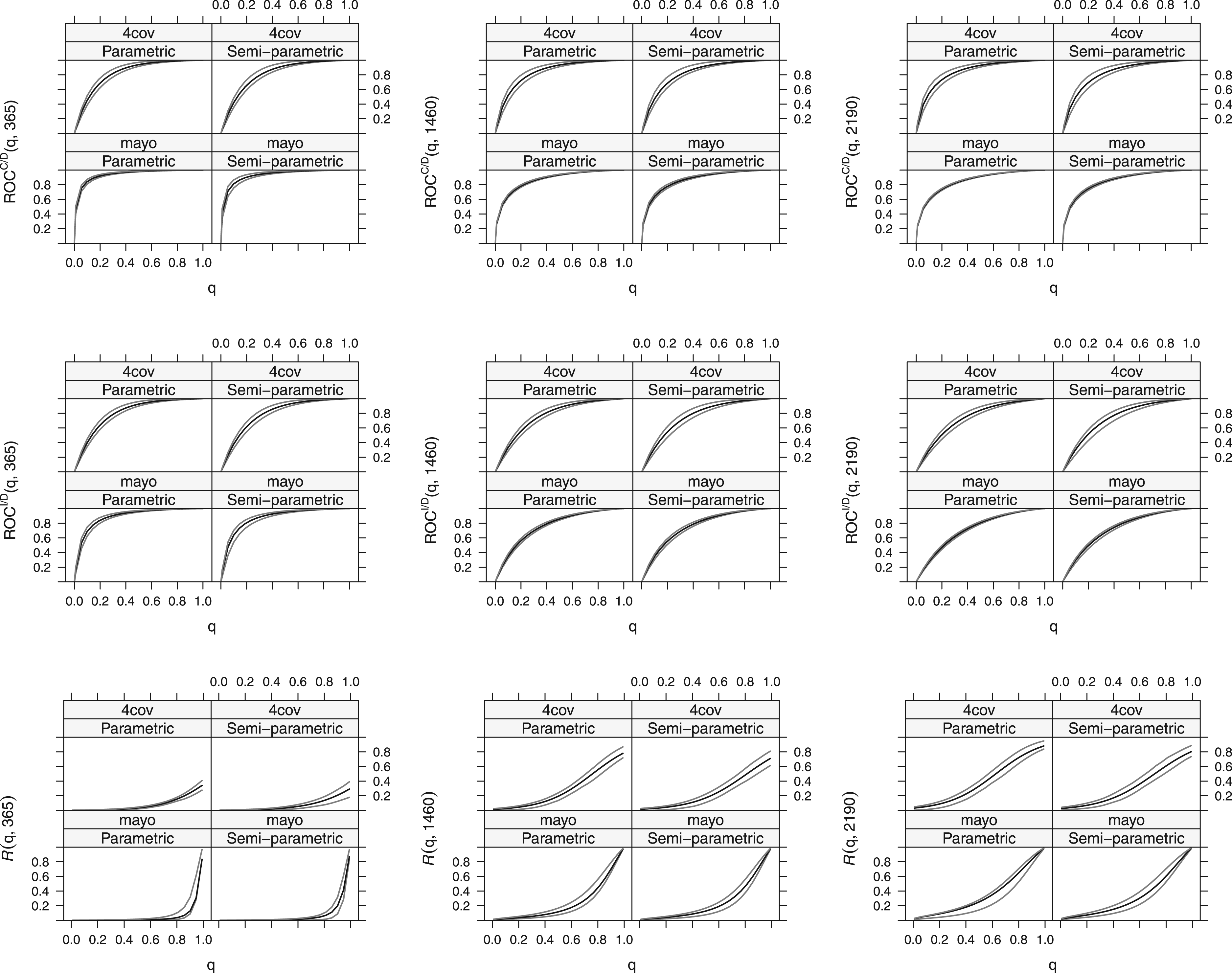
Figure 2 shows estimates and 95% confidence bounds of ${\mathrm{ROC}}^{\mathrm{C}/\mathrm{D}}(q,t)$ , ${\mathrm{ROC}}^{\mathrm{I}/\mathrm{D}}(q,t)$ and $R(q,t)$ for both markers at year 1, 4 and 6 from both the FP and SP copula models; here, the confidence bounds were constructed by joining pointwise CIs for each curve at various cut points of the marker quantile $q$ . It is clear that both models yield very similar fitted curves, with the confidence bounds being slightly wider for the SP model. All ROC curves indicate that both markers provide useful discriminating power for either outcome; in addition, the shapes of the confidence bounds of the ROC curves suggest that the corresponding population curves are at least approximately convex, which is a crucial feature for rational decision making, ²⁷ that implies that larger values of the marker are associated with a higher likelihood of outcome presence (e.g. Lloyd ²⁸ ). When it comes to comparing the discriminatory power of the two markers, mayo outperforms 4-cov since the corresponding ROC curves show estimates closer to the point $(0,1)$ , particularly for years 1 and 4; also, the three predictiveness curves of mayo appear to be steeper and closer to the point $(1,1)$ , allowing for better election of marker thresholds, which indicates that mayo provides higher predictive accuracy.

Figure 2.

Parametric and semi-parametric estimates, along with 95% confidence bounds, of receiver operating characteristic (ROC) ${}^{\mathrm{C}/\mathrm{D}}(q,t)$ , ${\mathrm{ROC}}^{\mathrm{I}/\mathrm{D}}(q,t)$ and $R(q,t)$ for markers 4-cov and mayo at times $t=365$ , $t=1460$ and $t=2190$ (days after registration).

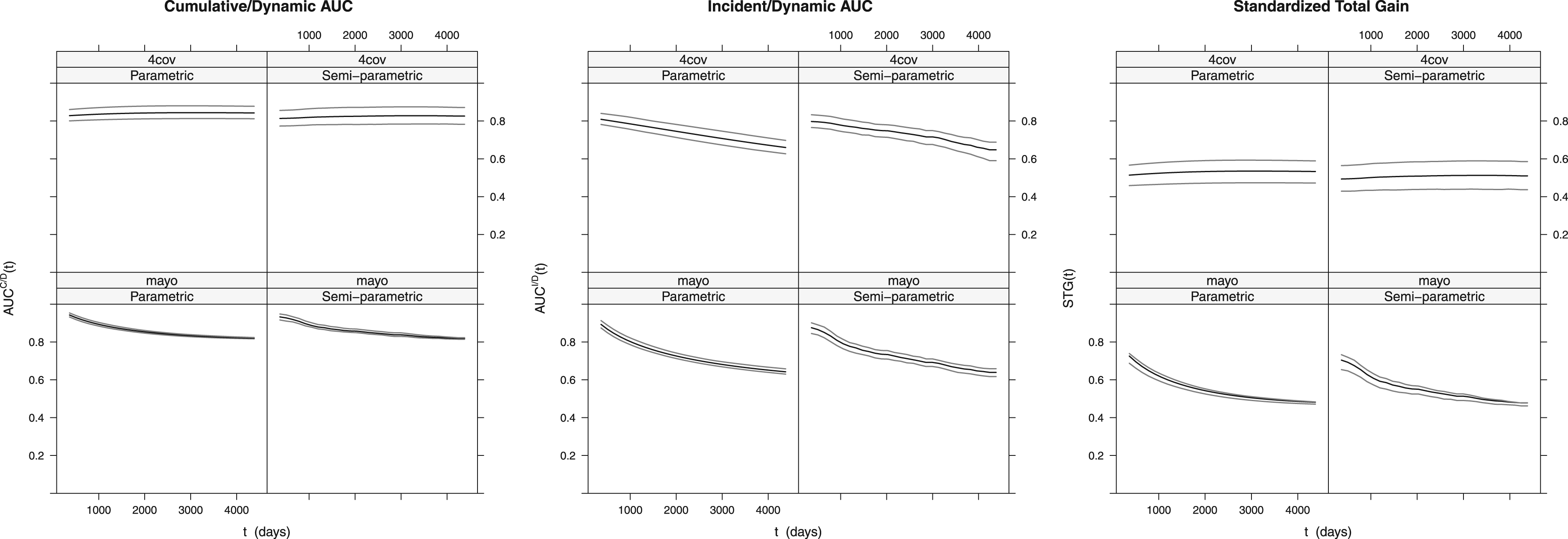
Figure 3 depicts estimates and 95% confidence bounds of ${\mathrm{AUC}}^{\mathrm{C}/\mathrm{D}}(t)$ , ${\mathrm{AUC}}^{\mathrm{I}/\mathrm{D}}(t)$ and $\mathrm{STG}(t)$ , for $t$ greater than one year, for 4-cov and mayo from the parametric and SP models; here, the confidence bounds were drawn by joining the pointwise CIs for each measure at different time points. The estimated functions appear somehow similar for both models, with the SP approach estimating wider confidence bounds, particulary for 4-cov. The cumulative/dynamic plots indicate that 4-cov keeps a fairly constant discriminatory rate for the status of the event occurring within time $t$ at around 0.8, and that the corresponding discriminatory rate of mayo decreases steadily with time to $0.8$ . The cumulative/dynamic plots show that the rate for discriminating the status of the event instantaneously occurring at time $t$ decreases steadily with time to 0.6 using either marker, with both markers yielding estimates of the AUC that exceed $0.75$ in the first 2000 days of the follow-up. More marked differences between both markers can be noticed in the plots of $\mathrm{STG}(t)$ , where the estimate for 4-cov appears fairly constant over time at around 0.5, whereas the estimate for mayo decreases steadily from around 0.7 to around 0.5, which supports the predictiveness superiority of mayo.

Figure 3.

Parametric and semi-parametric estimates, along with 95% confidence bounds, for area under the curve (AUC) ${}^{\mathrm{C}/\mathrm{D}}(t)$ , ${\mathrm{AUC}}^{\mathrm{I}/\mathrm{D}}(t)$ and $\mathrm{STG}(t)$ corresponding to markers 4-cov and mayo.

Discussion

In this paper, two new copula-based approaches to the representation of the joint model of marker and time to event were proposed, leading to parametric and SP characterizations of marker classification and predictivenes performance measures for survival outcomes. While the parametric representation of the model allows for the independent customization of each margin, such tailored specification is only required for the margin of the marker in the SP formulation, with the margin of the survival time being provided by a non-parametric estimator. In both models, the copula function encodes the dependence structure between the two random variables.

Maximum likelihood and a two-stage procedure were employed to obtain estimates in the parametric and SP specifications, respectively, and bootstrapping was performed for both approaches to obtain SEs and CIs. A strategy for choosing a copula from a set of candidates was based on assessing diagnostics plots for each conditional distribution. Simulation studies, which considered bias and RMSE for the assessment of the point estimators corresponding to classification and predictiveness measures, showed that both approaches performed well under different dependence and censoring scenarios.

The analysis of two markers from the PBC Mayo Clinic data illustrated the modeling process of the proposed methods, with both approaches producing similar results. This is the first study that displays ROC and predictiveness curves under the same framework. Meticulous investigation of the copula choice was necessary, and residuals plots for the conditional distributions offered a useful tool for the identification of the copula class with best fit for each marker. Unlike previous studies, where the methodologies were focused on point estimators mainly, the displays of the time-varying curves are by no means erratic (see e.g. Bansal and Heagerty, ¹ Kamarudin et al., ²⁹ and Viallon and Latouche ³⁰ ); in addition, the curves estimated here and their summaries showed CIs that are relatively narrow. Therefore, the methods developed in this paper provided an enhancement in the understanding of the classification and predictiveness characteristics of each marker.

The quantities that are used to compute a marker are registered at the beginning of the follow-up and tend to be fully observed, with the resulting observations being relatively easy to model parametrically by employing valid transformations, similar to the modeling of the usual parametric ROC analysis (e.g. Hanley ³¹ ). Linking a FP model for the marker with a non-parametric survival distribution for the time to event via the copula, in order to obtain the SP joint model, represents a convenient extension of the parametric joint model when univariate parametric models fail to give satisfactory fits to the survival margin, or when the survival time is subject to sampling schemes that lead to complex incomplete data structures such as interval censoring, which are difficult to model parametrically in the bivariate setting.

Although the copula-based methods do not lead to closed-form estimates of marker performance measures, they are appealing alternatives since the estimation procedures are for all measures within the same framework, and they consider all marker values and all failure and censoring times, with no information appearing to be lost. Previously proposed methods for estimating ${\mathrm{AUC}}^{\mathrm{I}/\mathrm{D}}(t)$ only, for instance, have mainly been based on smoothing techniques, and have proved to be highly influenced by data corresponding to earlier time points than $t$ , which can be considered a drawback since the focus is on assessing the prospective performance of a marker, not the retrospective. ²

While the copula-based methods presented in this study represent a convenient way to model the dependence between the marker and the survival time, they were formulated using four copula families only. Various bivariate models have been defined in terms of finite mixtures of copulas, leading to rich classes of joint models that can be employed to study complex dependencies^32,33; however, with the adoption of such mixture models, new problems arise, including the customization of the margins in each component, which might not be easy to address, particularly because the survival time is subject to various types of censoring.

In the cross-sectional data context, there has been interest in comparing ROC curves corresponding to two correlated markers. The three main comparison scenarios include ³⁴ : (a) Testing whether the two ROC curves are equal for all marker quantiles $q$ , (b) Testing whether the two AUC’s are equal, and (c) Testing whether the two ROC curves are equal at a particular marker quantile. In the survival outcome setting, Zhang and Shao ³⁵ developed vine copula-based algorithms to generate multivariate data for correlated markers, focusing mainly on the simulation for given concordance indexes. It is fair to say that extensions of the characterizations presented in this paper can be used in the three-dimensional framework by using vine copulas, to then elaborate the corresponding hypothesis tests for the various comparison scenarios. This, of course, warrants further research.