
Abstract
The distribution of time-to-event outcomes is usually right-skewed. While for symmetric and moderately skewed data the mean and median are appropriate location measures, the mode is preferable for heavily skewed data as it better represents the center of the distribution. Mode regression has been introduced for uncensored data to model the relationship between covariates and the mode of the outcome. Starting from nonparametric kernel density based mode regression, we examine the use of inverse probability of censoring weights to extend mode regression to handle right-censored data. We add a semiparametric predictor to add further flexibility to the model and we construct a pseudo Akaike’s information criterion to select the bandwidth and smoothing parameters. We use simulations to evaluate the performance of our proposed approach. We demonstrate the benefit of adding mode regression to one’s toolbox for analyzing survival data on a pancreatic cancer data set from a prospectively maintained cancer registry.
Keywords
Introduction
Mode regression (or modal regression) can be used to predict the mode of a continuous outcome conditional on covariates. The mode is of particular interest for highly skewed and multimodal data, where the mean and even the median can be unlikely values in a region of low density. They can be far away from the highest density region in the sense of Hyndman, 1 which we intuitively think of as the center of the distribution. In contrast, the mode can be seen as a more typical observation, an interpretation that might be rather appealing for applied scientists.
In this article, we extend mode regression to right-censored data. We imagine mode regression being a useful tool in analyzing time-to-event data with heavy skewness or multimodal data. In our application, we used the method to analyze survival times of pancreatic cancer patients. Pancreatic cancer is a highly fatal disease. It is often detected late and many patients die within the first year after diagnosis. In 2016, the one-year survival rate in Germany was 33% relative to survival in the general population. 2 While the underlying mechanisms are still unclear, some patients can have long survival times. The five-year survival rate in Germany was 9%. Overall survival was therefore expected to be right-skewed and results from mode regression were of interest.
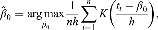
Existing approaches to mode regression are often based on kernel density estimation. Other approaches include direct derivative estimation and obtaining the mode via quantile regression among others.3,4 A summary of kernel density based mode regression methods can be found in a review by Chen. 5 Mode regression can be categorized into global and local mode regression. Local mode regression aims to model the relationship between covariates and multiple local maxima of the conditional density. This can be done by estimating the joint density of outcome and regressors with multivariate kernel density estimation and maximization of the density for fixed covariate values. 6 Continuous covariates are modeled without the need to specify an explicit functional form. This flexibility, however, also leads to reduced interpretability, since covariate effects cannot be summarized in a few numerical estimates, but rather have to be inspected visually. Global mode regression, on the other hand, is concerned with the relationship between covariates and the global maxima of the conditional density. Common approaches are based on minimizing expected loss. 7 Our method is based on Kemp and Santos Silva, 8 who proposed minimizing empirical loss by maximizing a one-dimensional kernel density estimator. Covariate effects were included with a linear predictor, which simplified interpretability in comparison to smooth modeling of covariate effects. Still, flexible modeling as an option is desirable in many situations, which is why we aim to include flexible modeling in our approach.
Mode regression falls into the class of distributional regression methods that have been developed in the last decades to analyze different measures than just the conditional mean in the regression setting. While methods like quantile regression, 9 expectile regression 10 and Generalized Additive Models for Location, Scale and Shape (GAMLSS) 11 can be used to analyze tail behavior and are particularly useful in heteroscedastic settings, mode regression is an alternative method to quantify effects on the center of the distribution. Mode regression is a useful alternative if the data or context imply that the expectation and the median are not estimands of interest.
The approach taken in this paper starts from linear mode regression proposed by Kemp and Santos Silva 8 and adds useful extensions. The first extension is the inclusion of semiparametric predictors, allowing for the flexible modeling of spatial and temporal information as well as nonlinear effects of continuous covariates. We use penalized splines (P-splines), as made popular by Eilers and Marx, 12 for inclusion of nonlinear effects in mode regression. By using the normal kernel, computation of the estimator given in Kemp and Santos Silva reduces to a weighted least squares problem, which allows direct inclusion of least squares methods like P-splines.
The second important component of our model is the inclusion of right-censored data with inverse probability of censoring (IPC) weights, which has been examined, for example, for local mode regression 13 and expectile regression. 14 The weights lead to an exclusion of every censored event time, while every uncensored event time is used with an increased weight in estimation.
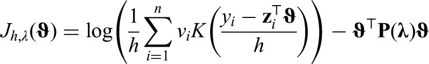
Kernel density estimation requires specification of the so-called bandwidth parameter, that controls smoothness of the estimated density. A bandwidth that is too small leads to an estimate with high variability, large bandwidths lead to smooth estimates with high bias. The importance of bandwidth selection for univariate kernel density estimation is often emphasized, and considerable research has been conducted to find an optimal selection method. 15 Specification of a bandwidth is also needed for kernel density based mode regression. Minimizing the asymptotic MSE has been proposed to choose the bandwidth for linear mode regression. 16 We examine the use of a pseudo Akaike’s information criterion (AIC) approach for selection beyond linear mode regression and uncensored data. We use the pseudo AIC to select both the bandwidth and the smoothness parameters of the penalized effects. Further, it can also be used as a model selection criterion.
In this article, we introduce and evaluate an extended mode regression model for right-censored data and use it to analyze pancreatic cancer data. In the section on “Method development,” we first summarize global mode regression based on kernel density estimation. We then extend the model to include semiparametric predictors and right-censored data. In the section concerning the “Analysis of overall survival of pancreatic cancer patients,” we present an analysis of survival times of pancreatic cancer patients, showing the potential benefits of using mode regression for survival analysis. In the section on “Numerical studies,” we show results from a simulation study, evaluating performance of our approach in comparison with GAMLSS.
Method development
Mode estimation and mode regression
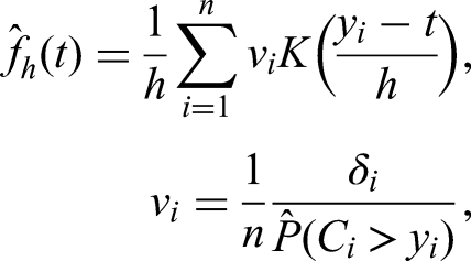
The (global) mode of a continuous random variable

There are various ways to estimate the mode, see for example Chacon
17
for an overview. Parzen
18
already considered mode estimation in his first publication on kernel density estimation. It turns out that simply maximizing the kernel density leads to a consistent estimator of the mode. For independent observations
Kemp and Santos Silva
8
as well as Yao and Li
16
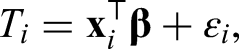
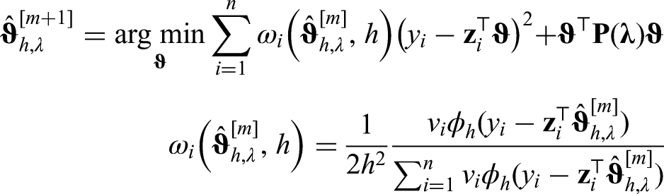
extended estimation of the mode to the regression setting. The framework is similar to usual linear least squares regression. Let

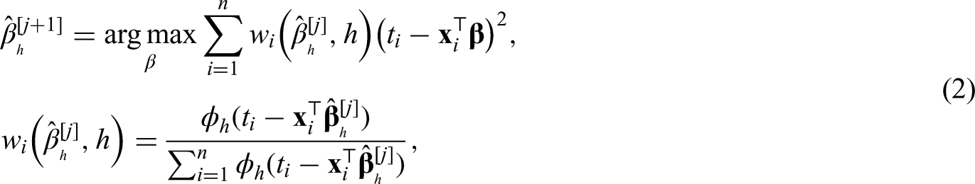
We propose two extensions to the regression approach formulated in equation (1). First, we allow right-censored data by adding IPC weights. Second, since iteratively weighted least squares are used, we can incorporate semiparametric predictors like P-splines, Gaussian Markov random fields and other flexibly modeled effects.
In the case of right-censored time-to-event data, estimation of the survival function is typically done with the Kaplan-Meier estimator.
19
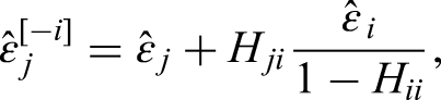
The estimator has many desirable properties like strong consistency and can be viewed as a nonparametric maximum-likelihood estimator.20,21 On the other hand, the Kaplan-Meier estimator is always a step function, even for continuous event times, which is an undesirable property. To remedy this, smoothing of the Kaplan-Meier estimator has been proposed, using Bezier curves or kernel smoothing among others.22,23 Kernel smoothing uses the step sizes of the Kaplan-Meier estimator

The weights
A potential problem that is encountered in using IPC is that some weights are lost if the longest observation(s) are censored. For mean regression, Zhou 25 added the lost weights to the longest observation to remedy this. In our experience, this problem is not as relevant for mode regression and a correction is not necessary, since the longest observations are usually far enough away from the mode of the distribution to have little to no effect on the estimates.
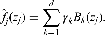
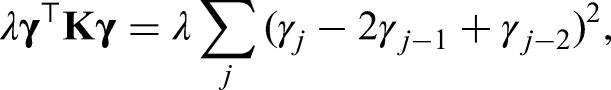
For the models in the previous sections, effects that could be modeled by simple and known functions were assumed. We prefer a more flexible approach by including a semiparametric predictor. A structured additive model as proposed in Fahrmeir et al.
26
allows us to capture effects more broadly. It is generally defined as

Hyperparameter selection
While the bandwidth

We implemented mode regression with the software R.
29
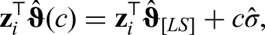
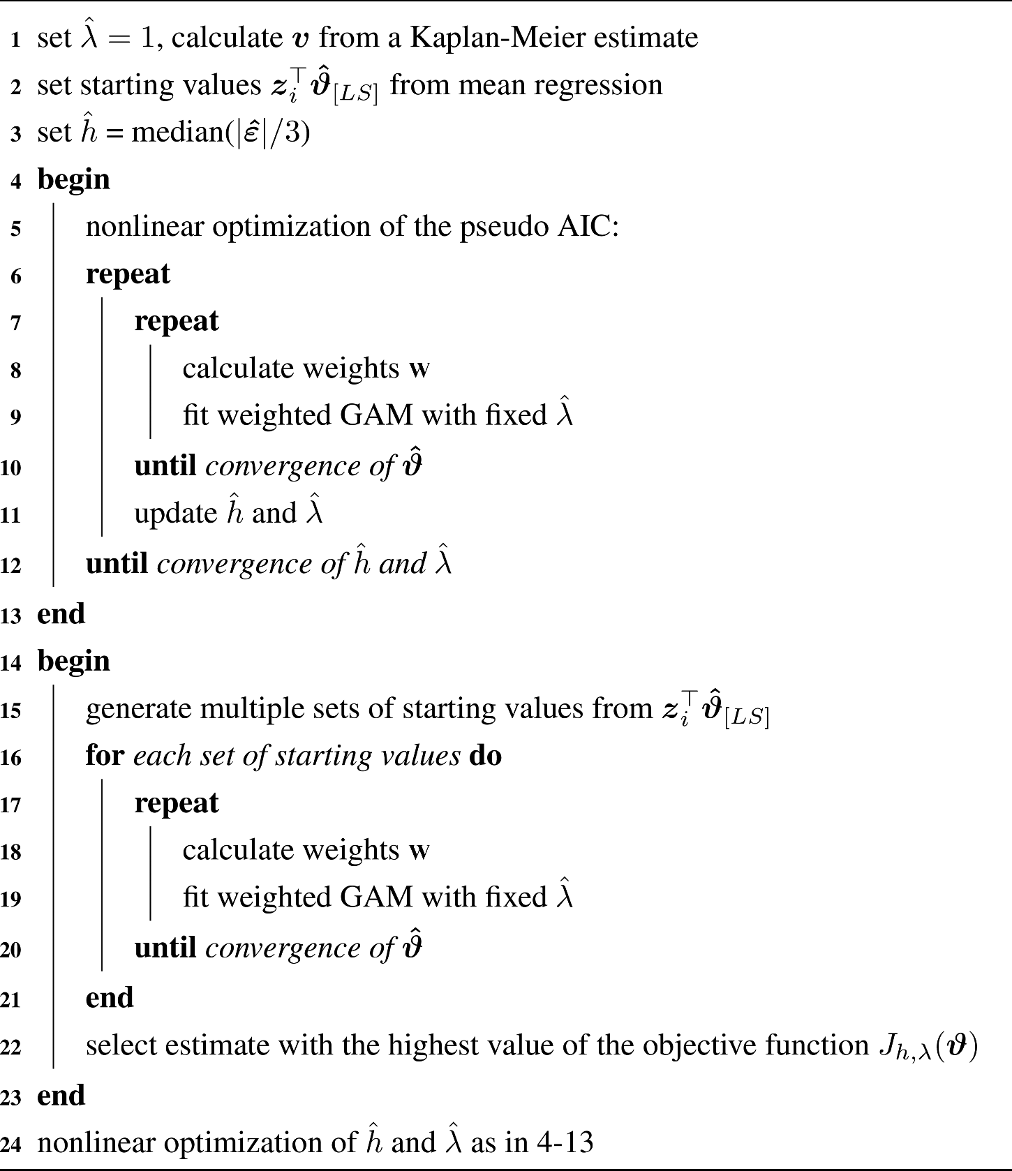
A summary of our algorithm is given in Algorithm 1. As a first step, starting values for hyperparameters and the mode are chosen. An arbitrary starting value of one is chosen for
Next, hyperparameters are selected. We use nonlinear optimization algorithms from the R package ”nloptr”.
30
After every update of the hyperparameters, the iteratively weighted GAM is refitted and the pseudo-likelihood is recalculated. After selection of hyperparameters, we calculate multiple starting values for the mode, since estimates can be sensitive to the initial values. We use 10 different sets of starting values in our simulations. Since for unimodal distributions, the difference between mean and mode is at most
We tested the computation time of the algorithm on our test system (CPU: AMD Ryzen 5 3600). Without P-splines, median computation time was 2.0 s (Q1: 1.7, Q3: 2.5) for 200 observations, 7.4 s (6.8, 8.2) for 1000 observations and 91.0 s (85.8, 96.4) for 5000 observations. With P-splines, median computation time was 6.8 s (5.2, 9.8) for 200 observations, 21.6 s (17.9, 28.4) for 1000 observations and 201.1 s (174.3, 355.6) for 5000 observations. More details can be found in the Appendix.
The computationally most demanding step was the optimization of hyperparameters. We found the number of optimization steps to be right-skewed and in some cases the number of required steps was quite large. In the interest of computational efficiency, we stopped maximization after 200 iterations. Details on the number of required steps can also be found in the Appendix.
Pseudo code of the implementation
Pseudo code of the implementation
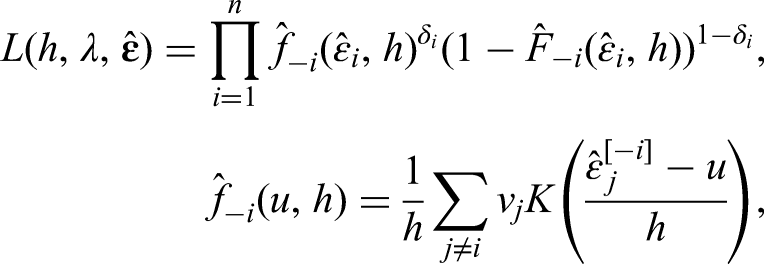
For the calculation of confidence intervals, we propose a nonparametric residual bootstrap. 32 It consists of the following steps in the case of uncensored data:
(1) Fit the mode regression model and calculate predictions
(2) Sample n times from the residuals with replacement, such that 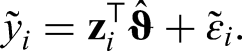
(4) Steps (2) and (3) are repeated k times and bootstrap estimates
(5) Bounds of the
We propose the following modification in the censored case: Since IPC weights indicate that an observation represents multiple unobserved event times, we use the IPC weights for sampling 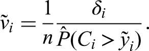
Analysis of overall survival of pancreatic cancer patients
We performed a retrospective exploratory analysis of overall survival and associated variables for pancreatic cancer patients. The goal of the analysis was a comparison of estimated regression coefficients between mode regression and parametric accelerated failure time (AFT) models.
Data source
The analyzed data set consisted of pancreatic cancer patients treated at the certified transregional pancreatic cancer center of the University Clinic for Visceral Surgery of the Pius Hospital Oldenburg. The Pius Hospital is an acute care hospital in the north-west of Germany and the University Clinic for Visceral Surgery performs a total of about 3000 inpatient and about 500 outpatient surgeries annually. The university clinic maintains a registry with prospective data collection, where the analyzed data originated from. The pancreatic cancer database lists 542 patients treated between 2010 and 2020, 158 of whom were included. We included patients with pancreatic adenocarcinoma as a histologic diagnosis who underwent surgical resection. Adjuvant therapy, that is, as supportive treatment after surgery, was given in accordance with standard guidelines. 33
The data that support the findings of this analysis are available on request from the corresponding author. The data are not publicly available due to privacy/ethical restrictions. The Pius-Hospital is an institution of the Catholic Church. In accordance with the Law on Data Protection of the Catholic Church in Germany, no ethics approval is needed for the retrospective analysis of anonymized data. Patients gave their informed consent for their data to be entered into the prospectively maintained cancer registry database of the Pius-Hospital Oldenburg, and for their data to be used in retrospective analyzes.
Variables
The endpoint was overall survival measured since diagnosis. Chemotherapy was dichotomized (yes/no). Contraindications (yes/no) prevented some patients from receiving chemotherapy. pT, pN, pM, and R status were determined from pathological analysis of tissue removed during surgery. The UICC classification 34 of pancreatic cancer was used to classify the tumors in stages I-IV. Lymph node ratio (LNR) is defined as the number of affected lymph nodes divided by the total number of examined lymph nodes. R status refers to the presence of residual tumor after surgery. Microscopic or macroscopic residual tumor at the edge of the resection is classified as R1 and R2, respectively. R0 (no residual tumor) can be further grouped by the distance between the resection margin and the tumor tissue. The circumferential resection margin (CRM) is negative if the distance is more than 1mm and positive else. Finally, patients who already suffered from other cancers at some point in their lives are described as having pre-existing cancer.
Descriptive statistics
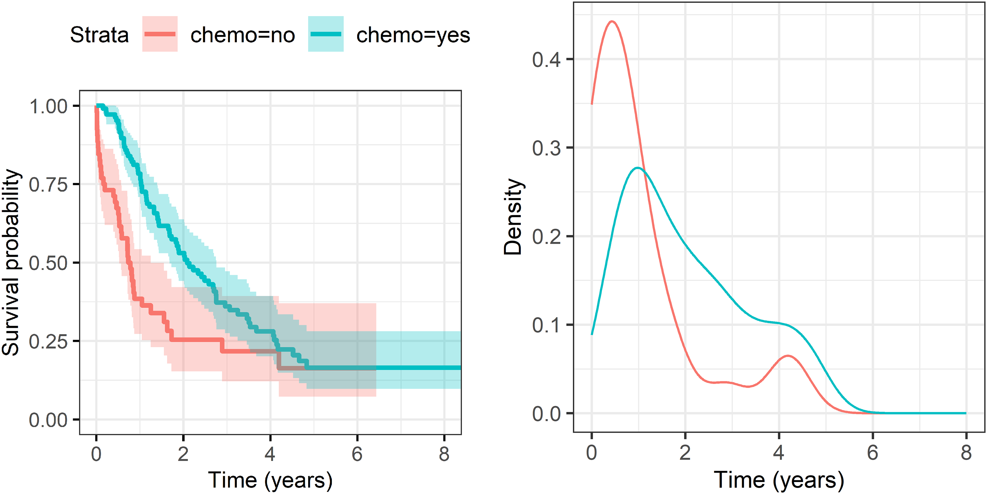
Baseline characteristics are shown in Table 1. Around two-thirds of patients received chemotherapy, in nine cases (6%) combined with radiotherapy. Most patients (113, 71.5%) had stage II pancreatic cancer. Survival times were censored in 43 cases (27%). Using reverse Kaplan-Meier estimation 35 (potential follow-up is censored by death), median potential follow-up was estimated to be 4.4 years (Q1: 2.8, Q3: 5.7). The Kaplan-Meier estimates of the survival times stratified by chemotherapy and the kernel smoothed densities based on the Kaplan-Meier estimates are shown in Figure 1. The bivariate analysis showed a positive association between chemotherapy and overall survival. Median survival was estimated at around 2.2 years (1.1, 4.1) for patients with chemotherapy treatment and 0.9 years (0.3, 2.5) without. The positive association with chemotherapy was particularly evident during the first year. Also, many patients died within the first year: estimated one-year survival was 77% with chemotherapy and 45% without. However, some patients survived a long time, the longest survival time was censored at 7.9 years. The density functions on the right side of Figure 1 show moderate and heavy skewness (1.1 with chemotherapy, 3.5 without), as well as signs of a second mode after 4 years of survival. Thus, there might be meaningful differences between results from mean, median and mode regression, suggesting practical relevance of mode regression for this group of patients.
Kaplan-Meier estimates stratified by chemotherapy with pointwise confidence interval (left) and smoothed density estimates (right) of survival times.
Descriptive statistics of the study population. Numbers are absolute (relative) frequencies, unless stated otherwise.
We fit a mode regression model and, for comparison, an AFT model assuming a parametric distribution as well as identically distributed residuals.
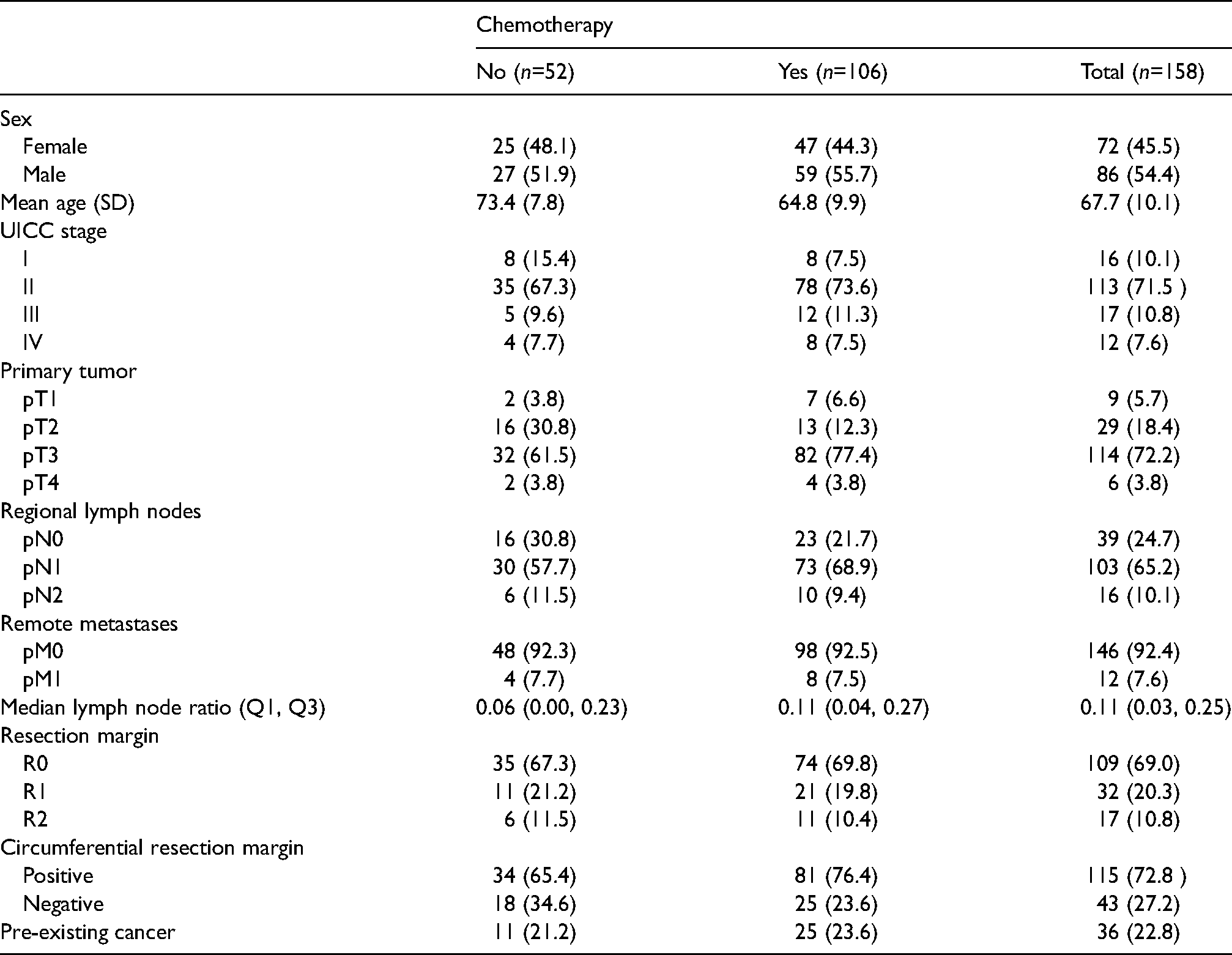
We began variable selection by including chemotherapy and LNR in our model, as they have been found to be the best predictors for long-term survival for pancreatic ductal adenocarcinoma. 36 It should be noted that for our observational data, the association between survival times and chemotherapy should be interpreted with care since treatment with chemotherapy might be subject to channeling bias. Treatment recommendations are usually given through an interdisciplinary tumor board. Various factors like expected survival chances, success of surgery, contraindications, general health and age might be considered. Boxplots for age in relation to chemotherapy and R status are depicted in Figure 2. 75% of patients without chemotherapy were 70 or older, while it were only 37% of patients with chemotherapy. Because of the potential confounding effect of age, we included it in our model as well and examined an interaction term after variable selection. In 16 cases, chemotherapy was not used because of contraindications. The S3 guidelines of the Association of the Scientific Medical Societies 33 define these as, for example, limited autonomy (ECOG score of 3 or higher), uncontrolled infections, cirrhosis of the liver (Child-Pugh score B or C) or severe coronary heart disease. Patients with contraindications were included in the analysis.
Boxplots of patients age seperated by chemotherapy and R status.
Inclusion of all other variables was determined by a best subset selection approach using the pseudo AIC defined in equation (4) as criterion. The model with the lowest pseudo AIC included an R status (residual tumor after surgery) in addition to chemotherapy, age and LNR. After variable selection, we added an interaction term between chemotherapy and age, but elected not to include the term in the final model due to fairly high standard errors for both the mode regression and AFT model. At this point, we compared the linear model with models using P-splines for age and LNR. The model with linear associations had the lowest pseudo AIC. However, we also show results from a model using P-splines to estimate the association with age to illustrate our method in more detail.
Parameter estimates from the fitted models can be found in Table 2, along with estimates from a parametric AFT model, using the same variables. The Weibull distribution was assumed since it showed the best parametric fit (determined by graphical inspection of residuals). The estimated nonlinear association between age and survival is shown in Figure 3.
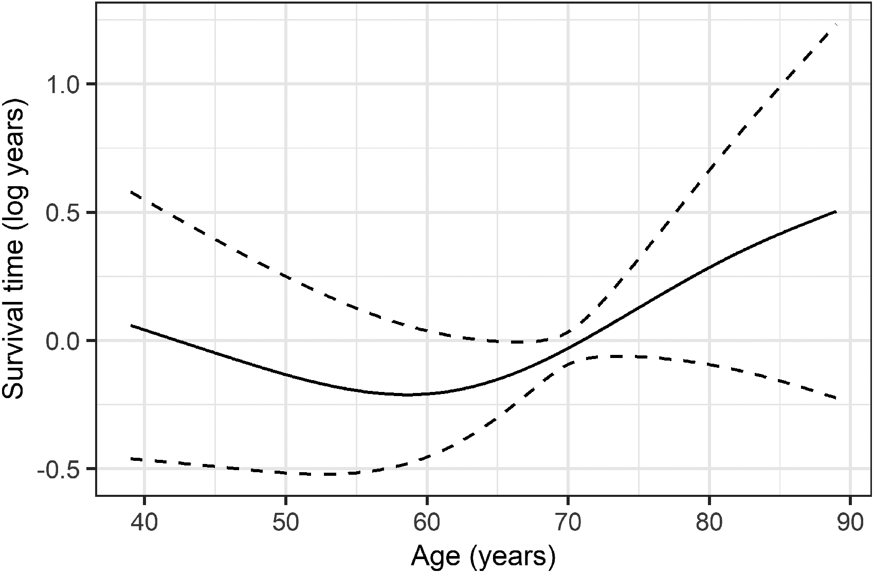
Estimate (solid line) and 95% confidence interval (dashed lines) for the relationship between age and mode of the log survival time.
Linear parameter estimates (95% confidence intervals) for mode regression and the Weibull model.
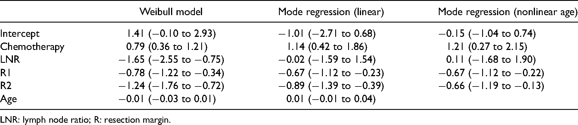
LNR: lymph node ratio; R: resection margin.
The estimated association between chemotherapy and the log survival time was positive and smaller for the Weibull model (0.79, 95% CI: 0.36–1.21) in comparison to linear mode regression (1.14, 0.99–2.37). Point estimates of the linear mode regression model were fairly close to the estimates for the nonlinear model for all variables except age. Microscopic and macroscopic residues (R Status) were found to be associated with shorter survival time for all models, but more so for the Weibull model. The nonlinear association between age and log survival time was slightly negative up to 59 years and positive after. In comparison, no association was estimated between age and log survival time for linear mode regression. LNR had a negative association with survival for the AFT model, but no association was found between survival and LNR for mode regression.
As shown in this analysis, the estimates from mode regression and AFT models can differ substantially. However, differing estimates are not too surprising, first, because the survival time might be multimodal and violate the Weibull assumption and, second, the estimated parameters have different interpretations. For mode regression, the estimates relate to changes of the modal log survival time. Receiving chemotherapy was estimated to increase the modal log survival time by 1.14 log years. For the AFT model, chemotherapy was estimated to increase the log survival time by 0.79 log years. The AFT model estimate can be interpreted as a location shift for the whole distribution. The differing estimates for chemotherapy are also in line with the bivariate Kaplan-Meier estimates, showing a stronger association for patients dying within the first year and a weaker association for patients with longer survival times. While a constant location shift is assumed for the AFT model, mode regression is able to detect associations that are specific for a patient dying within the first year.
Simulation setup
We compared our proposed mode regression method with AFT and GAMLSS models as well as our bandwidth selection with the plug-in bandwidth approach in a simulation study. We aimed to study the properties of our estimator in realistic finite sample scenarios. We started with a base scenario derived from the data and results of the analysis of pancreatic cancer patients and generated different scenarios through modifications of the base case, like the amount of censoring, signal-to-noise ratios and choice of event-time distributions.
The base scenario was developed using AFT models of our pancreatic cancer data as starting points. For the censoring time of overall survival, we found the log-logistic AFT model to be the best parametric fit (determined by graphical inspection of residuals). The censoring time was estimated with log(T) was Gumbel distributed with a scale of 0.97. The signal-to-noise ratio was 30%.
We chose one binary and one metric nonlinear covariate for the base model. Coefficients were chosen in agreement with the observed signal-to-noise ratio. An intercept was chosen such that the share of censoring was 27%, as observed in the pancreatic cancer data. Finally, we also added heteroscedasticity, such that the scale was increased or decreased by up to one-third, depending on the values of the covariates. The resulting event time model was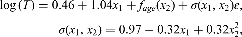
In addition to the base scenario, we simulated several scenarios with variations from the base case. An overview is given in Table 3. Share of censoring was varied (50% and uncensored data), as well as the signal-to-noise ratio (15% and 60%). Covariate influence on C was introduced, violating an assumption of our model. Linear trends were used instead of nonlinear trends. We also replaced the Gumbel distribution with a logistic distribution while retaining the variance. Each scenario was simulated with 200 and 500 observations and 200 repetitions.
Summary of the simulation setup and variations.
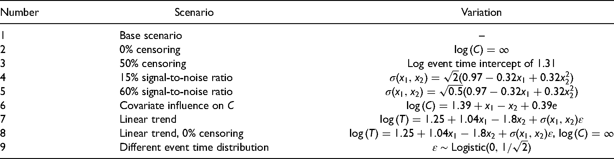
Summary of the simulation setup and variations.
We compared our proposed mode regression approach with mode regression using plug-in bandwidth selection described in Yao and Li 16 (only for uncensored data), with two GAMLSS and one parametric AFT model. In short, GAMLSS is a parametric model which allows modeling parameters other than just the location. In this case, the GAMLSS models assumed covariate influence on the variance, while for the AFT model a constant variance was assumed. For the first GAMLSS model, we assumed a Weibull distribution for the event time (only correct for scenarios 1–8), the second incorrectly assumed a log-normal distribution. A Weibull distribution was also used for the AFT model. All models assumed the proper linear relationships in scenarios 8 and 9 and used P-splines in all appropriate cases (nonlinear trends in scenarios 1–7, estimation of the scale).
To evaluate point estimates, predictions were made for observations on a regular grid with 100 points between zero and one for 
We used the software R 4.0.2 29 for all simulations. The package GAMLSS 11 was used for the parametric models. Our implementation of mode regression has been published in a dedicated R package, 37 our simulation code is available on request. Random seeds were used to generate pseudo random numbers and saved to allow reproducibility.
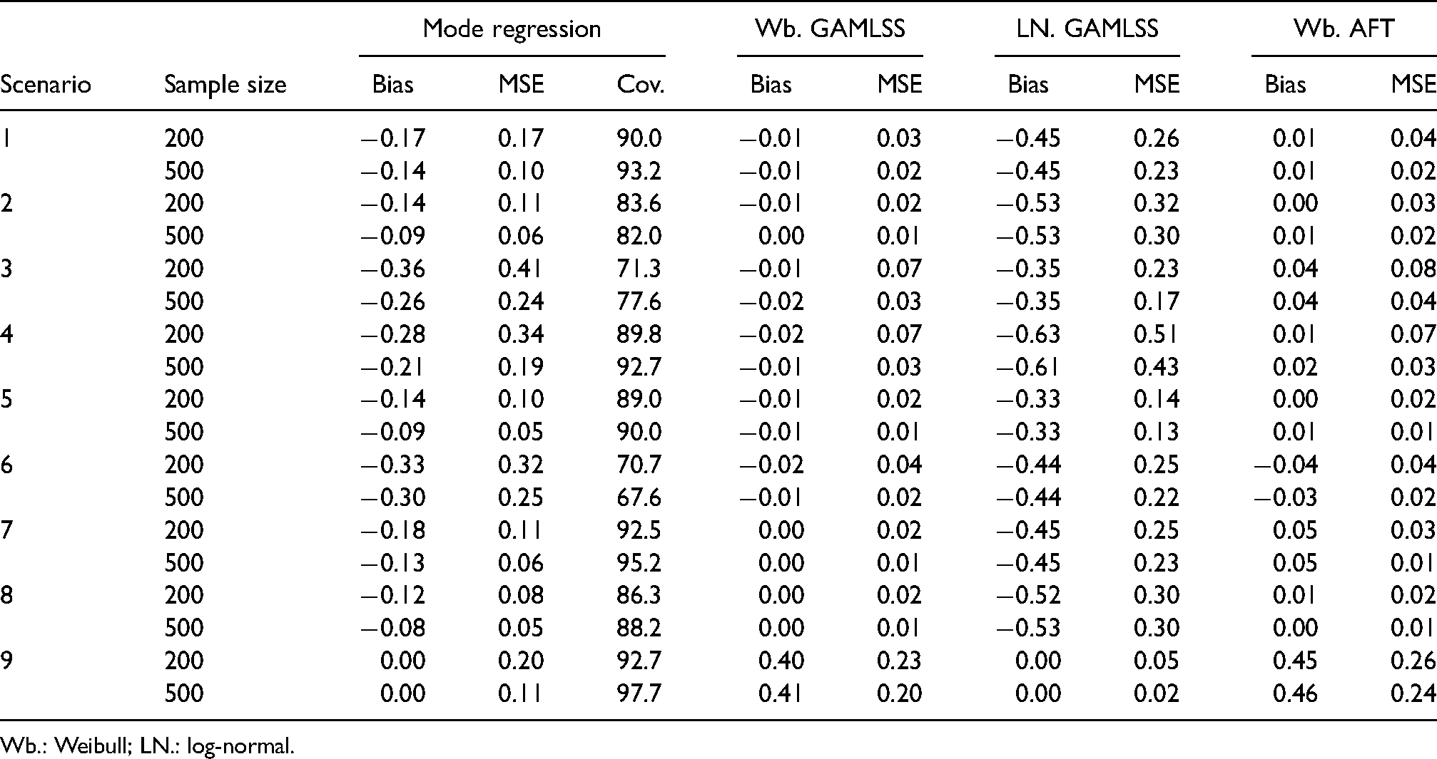
Our simulation results are shown in Table 4. In general, the results showed good performance of mode regression. Bias and MSE were for the most part within the bounds of the parametric GAMLSS models with correct and partially incorrect assumptions. Further, bias and MSE were reduced with increasing sample size, indicating possible consistency. The empirical coverage of the estimates did not reach the desired confidence level but was close to the level in many scenarios. Further details are given below.
Bias, mean squared error (MSE) and mean empirical coverage (Cov.) in different simulation scenarios.
Bias, mean squared error (MSE) and mean empirical coverage (Cov.) in different simulation scenarios.
Wb.: Weibull; LN.: log-normal.
Mode regression had a negative bias in every scenario except one and was always reduced with increasing sample size. In the base case (scenario 1), the bias was
The MSE showed similar trends as the bias. In most scenarios, mode regression had a larger MSE than the parametric model with the correct distribution and lower MSE than the model with the incorrect distribution. However, the MSE of mode regression was closer to the incorrect GAMLSS model than the bias. In the base case, the MSE was 35% and 57% lower than the MSE of the log-normal GAMLSS for n = 200 and n = 500. In comparison, the bias was 62% and 69% lower. The poorest results for mode regression were in scenario 3 (50% censoring) and scenario 6 (covariate influence on censoring). Bias was close to the log-normal GAMLSS and MSE was larger than the MSE of the parametric models. Bias and MSE were also reduced with increasing sample size in both scenarios. The MSE was close to the log-normal GAMLSS for 500 observations.
As a comparison, we also performed mode regression with the plug-in bandwidth approach in scenario 8 (uncensored data, linear trends). Bandwidth selection with the pseudo-likelihood and the plug-in approach performed equally well, the MSE was 0.09 for the plug-in approach at 200 observations, at 500 observations, it was 0.05. In comparison, the MSE of the GAMLSS model with correct assumptions was between 0.02 and 0.01 for 200 and 500 observations. The bias of the pseudo-likelihood and plug-in approach were also similar to each other.
The residual bootstrap resulted in empirical coverages below 95%. However, coverages were above 85% in most scenarios. Scenario 2 (uncensored data, nonlinear trends), scenario 3 (50% censoring) and scenario 6 (covariate influence on censoring) had the lowest coverage. For scenarios 3 and 6, this was in agreement with the reported elevated bias and MSE.
We extended mode regression with IPC weights and semiparametric predictors, resulting in a flexible method for time-to-event analysis. Mode regression allows us to estimate the conditional mode, which is a more appropriate location measure for heavily skewed or multimodal data than the mean or median. The conditional mode might also be a more intuitive measure than the hazard ratio, which has been criticized for being less appealing for patients and doctors than direct interpretation of the survival time. 38 While direct interpretation of the survival time is quite intuitive, similar to acceleration factors in AFT models, we have avoided direct interpretation of the raw survival time in our application and focused on the log-survival time instead. That is because transformations of the estimates to the raw survival time require additional information or assumptions. A partial remedy might be the use of the softplus response function, a combination of the exponential response function and the identity, as proposed by Wiemann and Kneib. 39 The transformation assumes a multiplicative association for shorter survival times and a smooth transition to a linear association after some specified time. While the multiplicative part of the survival time would still be hard to interpret, changes after the transition to the identity could be interpreted linearly and a transformation would be unnecessary.
The main caveats of other conventional methods for survival analysis are, however, their basic assumptions. This could be the expected proportionality of hazards or the choice of a parametric distribution for the response. Violations of these assumptions can lead to biased results, for example, the average hazard ratio is underestimated for converging hazard rates when the proportional-hazards model is used. 40 By using mode regression, we are able to circumvent these assumptions and are therefore in less danger of obtaining biased results.
The choice to use mode regression should depend mostly on the research question. For pancreatic cancer, mode regression is suitable for the special research interest in patients who die within the first year. Results from our analysis of pancreatic cancer suggested a stronger association of chemotherapy with the mode of overall survival than the association estimated in a parametric AFT model.
In our simulation study, bias and MSE were shown to be mostly bound between parametric models with correct and incorrect distributional assumptions. We have seen a strong difference between the two in such a way that a correct selection of the distribution of the response is crucial for the usability of the corresponding regression coefficients. While mode regression never outperforms a parametric model with correct assumptions, its results are far closer to a correctly assumed model than to a parametric model with false assumptions. The simulations further showed that bias and MSE were reduced with increasing sample size. Although residuals were not identically distributed in our simulations, we used a residual bootstrap for calculation of confidence intervals. Empirical coverages were below 95%, but above 85% in most scenarios. The scenarios with covariate influence on the censoring time and a larger share of censoring had elevated bias and MSE and the empirical coverage was much lower than in other scenarios. For heavy censoring, sample sizes larger than 500 might be necessary. For uncensored data, results from mode regression with the pseudo-likelihood were similar to the plug-in approach, which has been shown to be consistent. 16
A further area that would benefit from additional research is model selection. While we used the pseudo AIC to perform model selection in our application to pancreatic cancer survival and the chosen variables agreed with our general intuitions about the variables, performance of model selection criteria should be studied in more detail.
Footnotes
Acknowledgements
We thank Thomas Kneib for helpful discussions and exchange of ideas. We also would like to thank two anonymous referees for their valuable comments that led to considerable improvements of this article.
Declaration of conflicting interests
The author(s) declared no potential conflicts of interest with respect to the research, authorship, and/or publication of this article.
Funding
We gratefully acknowledge financial support from the German Research Foundation (DFG) grant SO1313/1-1 project “Distributional Regression for Time-to-Event Data.”