Approximate Bayesian computation design for phase I clinical trials

Abstract

In the development of new cancer treatment, an essential step is to determine the maximum tolerated dose in a phase I clinical trial. In general, phase I trial designs can be classified as either model-based or algorithm-based approaches. Model-based phase I designs are typically more efficient by using all observed data, while there is a potential risk of model misspecification that may lead to unreliable dose assignment and incorrect maximum tolerated dose identification. In contrast, most of the algorithm-based designs are less efficient in using cumulative information, because they tend to focus on the observed data in the neighborhood of the current dose level for dose movement. To use the data more efficiently yet without any model assumption, we propose a novel approximate Bayesian computation approach to phase I trial design. Not only is the approximate Bayesian computation design free of any dose–toxicity curve assumption, but it can also aggregate all the available information accrued in the trial for dose assignment. Extensive simulation studies demonstrate its robustness and efficiency compared with other phase I trial designs. We apply the approximate Bayesian computation design to the MEK inhibitor selumetinib trial to demonstrate its satisfactory performance. The proposed design can be a useful addition to the family of phase I clinical trial designs due to its simplicity, efficiency and robustness.

1 Introduction

In oncology research, a phase I clinical trial often aims to determine the maximum tolerated dose (MTD), which is typically defined as the dose with the dose-limiting toxicity (DLT) probability closest to the target toxicity rate. ¹ In the development of new drugs, phase I clinical trials play an essential role because the selected MTD will be further investigated in the subsequent phase II or III trials. Misidentification of the MTD would lead to an unreliable conclusion and may even cause termination of a trial immaturely. As a result, this leads to a waste of abundant resources as well as exposing patients at excessively toxic doses, which violates the ethical principle. Moreover, as the first-in-human study, subjects available for a phase I trial are rather limited, and the sample size is typically around $35$ , ² and thus it is challenging to identify the MTD with such a small sample size.

Various phase I trial designs have been proposed with the goal to determine the MTD both efficiently and accurately. Depending on whether to adopt a model assumption on the dose–toxicity curve or not, these designs can generally be classified into two branches: the algorithm-based (model-free or curve-free) and the model-based (often imposing a parametric model assumption) approaches. In the algorithmic family, the $3+3$ design ³ is the most commonly used one for phase I oncology trials due to its simplicity and conservativeness. ⁴ However, the $3+3$ design has also been criticized for its poor performance due to inefficient use of the data. Alternatively, a variety of model-free designs have been developed to improve the trial efficiency in determining the MTD. Gasparini and Eisele ⁵ presented a curve-free method in which the probabilities of toxicity are directly modeled as an unknown multidimensional parameter. Ivanova et al. ⁶ proposed a cumulative cohort design (CCD) where the dose escalation or de-escalation criterion is based on the Markov chain theory. To enhance the trial safety, the modified toxicity probability interval (mTPI) design is proposed using a unit probability mass. ⁷ Under the Bayesian framework, Liu and Yuan ⁸ developed the Bayesian optimal interval (BOIN) design by minimizing the probability of incorrect dose allocation. Yan et al. ⁹ proposed the keyboard design by partitioning the toxicity probability scale into more and shorter intervals. Enlightened by the uniformly most powerful Bayesian test, ¹⁰ Lin and Yin ¹¹ developed the uniformly most powerful Bayesian interval (UMPBI) design for phase I dose-finding trials.

Along the line of directly modeling the dose–toxicity curve, many model-based phase I designs have been proposed. The continual reassessment method (CRM)^12,13 is the most popular model-based design, which typically adopts a single unknown parameter to link the true and the prespecified toxicity probabilities at different dose levels. Cheung and Chappell ¹⁴ extended the CRM by incorporating weights to account for the late-onset toxicity outcomes. Another extension of the CRM focuses on modeling bivariate competing outcomes. ¹⁵ By incorporating the Bayesian model averaging (BMA) approach, Yin and Yuan ¹⁶ developed the BMA-CRM to overcome the arbitrariness of skeleton specification (i.e., the prespecified toxicity probabilities of all doses) and thus enhance the model robustness. Further extensions of the CRM include O’Quigley and Paoletti ¹⁷ Yuan et al. ¹⁸ and Wages et al. ¹⁹ among others. Due to safety concerns, the escalation with overdose control (EWOC) ²⁰ is designed to locate the MTD subject to the constraint that the predicted proportion of patients receiving overdoses does not exceed a specified threshold. Without assuming any parametric model, the nonparametric overdose control design is developed to enhance model robustness with little sacrifice on trial efficiency. ²¹ For more detailed discussions on the characteristics of various phase I designs, refer to Zhou et al. ²²

Our work is motivated by a phase I trial on the MEK inhibitor selumetinib in children with progressive low-grade gliomas (LGG). ²³ There were three candidate doses in the trial: 25, 33, and 43  mg/ ${\mathrm{m}}^2$ /dose bis in die. The target DLT rate was $\varphi =0.25$ . Originally, the trial adopted the likelihood-based modified CRM using a two-parameter logistic model based on dosages adjusted for the body surface area. However, because the prior information on the dose–toxicity curve is very limited at the phase I trial stage, model-based designs might be at risk of violating the parametric assumption, which undermines the efficiency of the dose-finding procedure. Moreover, with only three doses under investigation, a parametric model may not fit the data well. On the other hand, if we choose an algorithm-based method to select a dose for an incoming cohort of patients, most of the existing methods only consider the data collected at the current dose level, which weakens the efficiency of the design by not fully using all the cumulative data in the trial thus far. For example, a typical interval design determines the next dose level solely based on the data from the current dose level.

To alleviate the risk of model misspecification and utilize all the available information accrued in the trial, we develop an approximate Bayesian computation (ABC) design to identify the MTD. By adopting the idea from the approximate Bayesian computation sampling methods, ²⁴ the ABC design generates the weighted posterior samples based on all the available data without any complex formulas and dose–toxicity model assumptions. Based on the weighted samples, decisions among dose escalation, de-escalation, or retaining the current dose are made for each cohort. In this way, our method avoids introducing any explicit dose–toxicity model, yet can utilize the cumulative information from all dose levels when selecting the next dose level. Extensive simulation studies demonstrate that the ABC design is efficient compared with the state-of-the-art methods, while it is robust due to its model-free or curve-free feature. The main contributions of our work are twofold. First, we propose a novel phase I design which is robust and efficient under different scenarios. Second, by incorporating the ABC sampling into the phase I design, our work can be easily extended to other more complicated phase I trials.

The rest of the paper is organized as follows. In Section 2., we introduce the ABC design for dose finding in phase I clinical trials. We present the simulation studies to evaluate the operating characteristics of the ABC design and compare it with several well-known phase I designs in Section 3. An application to the phase I trial of the MEK inhibitor selumetinib is provided in Section 4. The paper is concluded with a brief discussion in Section 5.

2 Methodology

Suppose that a phase I clinical trial aims to investigate $K$ dose levels with the corresponding DLT rates $p_1<\cdots <p_K$ . The target toxicity rate is denoted as $\varphi$ . After enrolling and treating the first $n$ cohorts of patients, the current dose level is denoted by $d_n$ . Thus far, we observe the cumulative data $Y_n=\{y_k{\}}_{k=1}^K$ and $M_n=\{m_k{\}}_{k=1}^K$ , where $y_k$ represents the number of observed DLTs and $m_k$ represents the number of patients treated at dose level $k$ .

The main goal of the ABC design is to adopt all the available information when deciding the dose level for the next cohort without imposing any explicit dose–toxicity model assumption. In the Bayesian framework, we first assign a prior $\pi (p_1,\dots ,p_K)$ on $\{p_k{\}}_{k=1}^K$ , and then we can update the posterior distribution of $(p_1,\dots ,p_K)$ as

$$\pi (p_1,\dots ,p_K|Y_n,M_n)\propto P(Y_n|\{p_k{\}}_{k=1}^K,M_n)\pi (p_1,\dots ,p_K),$$

where $P(Y_n|\{p_k{\}}_{k=1}^K,M_n)$ is the likelihood function. Based on the posterior distribution, the next dose level can be selected accordingly. The major difficulty lies on how to choose a suitable and simple prior $\pi (p_1,\dots ,p_K)$ while taking the monotonicity constraint $p_1<\cdots <p_K$ into account. The dilemma is that a parametric model assumption typically undermines the robustness of the design, while due to the monotonicity constraint, the specific form of the prior $\pi (p_1,\dots ,p_K)$ without such a parametric model assumption can be complicated. The unusual complexity of the prior would also diminishes the flexibility of the design. Further, it causes difficulties in calculating the posterior distribution as well as the subsequent Bayesian inference.

2.1 Approximate Bayesian computation

To circumvent the aforementioned problem, we adopt the idea from the ABC sampling methods. ²⁴ The ABC methods are typically used to handle complex models, where the evaluation of the likelihood function is computationally costly or elusive. In such cases, the Bayesian inference with a closed-form posterior distribution is prohibitive. The ABC methods bypass the evaluation of the likelihood function with Monte Carlo simulations.

Suppose that we are interested in obtaining the posterior samples of parameter $\theta$ given the data $D$ and prior $\pi (\theta )$ . A simple ABC method, known as the ABC rejection algorithm, ²⁵ is described as follows:

Draw a sample $\hat{\theta }$ from the prior $\pi (\theta )$ .

Given the sample $\hat{\theta }$ , generate data $\hat{D}$ under the likelihood model $P(D|\theta )$ using the prior predictive distribution.

If the generated data $\hat{D}$ is close to the observed data $D$ under some prespecified distance measure, we keep the sample $\hat{\theta }$ as the posterior sample; otherwise, the sample is rejected and discarded.

The procedure is repeated for a large number of times to obtain adequate posterior samples of $\theta$ .

In the phase I trial setting, the evaluation of the likelihood is rather simple, while the prior model is complicated without a closed form due to the monotonicity constraint. On the other hand, the monotonicity constraint is can be naturally incorporated when we implement Monte Carlo simulations. For example, we can first generate the samples without any constraint and then sort them in an ascending order to preserve the monotonicity in the prior samples of $\{p_k{\}}_{k=1}^K$ . In Section B of the Supplemental Appendix, we present a toy example of using different approaches to sampling multivariate random variables under the monotonicity constraint, which shows that Monte Carlo simulation gives a simple and efficient way to solve such monotonically constrained sampling problem. Therefore, the ABC methods provide a very simple solution to obtain the constrained posterior samples of $\{p_k{\}}_{k=1}^K$ in a Monte Carlo manner.

2.2 Optimal dose selection

With the ABC rejection algorithm in hand, we are still not ready to obtain the posterior samples of $\{p_k{\}}_{k=1}^K$ for a phase I trial. The main challenge lies in the low efficiency of the ABC rejection method, because its acceptance rate can be very low which makes the procedure rather slow to obtain an adequate number of posterior samples for reliable and robust inference. Moreover, under the ABC rejection method, all the $\hat{\theta }$ ’s leading to the generated $\hat{D}$ ’s inconsistent with the observed data $D$ are equally discarded. However, even the discarded $\hat{\theta }$ ’s can still provide some useful information about the posterior distribution. For example, some generated data $\hat{D}$ ’s may be very different from the original data $D$ , while some may only moderately deviate from $D$ , and thus we should not blindly discard the corresponding $\hat{\theta }$ ’s without discrimination.

Considering both issues as mentioned above (the low acceptance rate and equally discarding unqualified posterior samples), we propose to adopt the weighed ABC sampling for a phase I trial as follows:

Select a suitable prior distribution $\pi (p_1,\dots ,p_K)$ and a distance measure ${\rho }_h(\cdot ,\cdot )$ .

Generate the prior samples $\{p_{k,(j)}{\}}_{k=1}^K$ for a large number $J$ times from $\pi (p_1,\dots ,p_K)$ .

Given the prior samples $\{p_{k,(j)}{\}}_{k=1}^K$ , we generate the corresponding data, $Y_{n,(j)}=\{y_{k,(j)}{\}}_{k=1}^K$ with $y_{k,(j)}\sim \mathrm{Binom}(p_{k,(j)},m_k)$ .

Based on the generated data $\{Y_{n,(j)}{\}}_{j=1}^J$ , the weight for each sample $\{p_{k,(j)}{\}}_{k=1}^K$ can be obtained as $w_{(j)}={\rho }_h(Y_{n,(j)},Y_n)$ , where $Y_n=\{y_k{\}}_{k=1}^K$ is the originally observed data.

Use the weighted samples $\{(w_{(j)},\{p_{k,(j)}{\}}_{k=1}^K){\}}_{j=1}^J$ as the posterior samples for statistical inference.

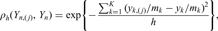
Motivated by the Gaussian kernel, we choose the distance measure as

$${\rho }_h(Y_{n,(j)},Y_n)=\exp \{-\frac{\sum _{k=1}^K(y_{k,(j)}/m_k-y_k/m_k{)}^2}{h}\},$$

where $h$ is the bandwidth and its selection will be discussed in Sensitivity Analysis Section.

The above procedure is essentially referred to as the ABC importance sampling when the proposal density is taken as the prior distribution. ²⁶ Therefore, it is guaranteed that the weighed samples are approximately generated from the posterior distribution. This weighted procedure overcomes the low acceptance rate problem of the ABC rejection method, because it adopts all the prior (weighted) samples for the posterior inference. We then estimate the toxicity rate for dose level $k$ as

$${\hat{p}}_{n,k}=S(\{p_{k,(j)}{\}}_{j=1}^J,\{w_{(j)}{\}}_{j=1}^J),$$

where $S(\cdot ,\cdot )$ can be any function yielding a reasonable estimator ${\hat{p}}_{n,k}$ . By default, we take $S(\cdot ,\cdot )$ as the weighted median due to its robustness. The weighted median function is the $50$ th weighted percentile of $\{(w_{(j)},p_{k,(j)}){\}}_{j=1}^J$ obtained as follows:

• Sort $\{p_{k,(j)}{\}}_{j=1}^J$ in an ascending order to obtain $\{{\tilde{p}}_{k,(j)}{\}}_{j=1}^J$ attached with the corresponding weights $\{{\tilde{w}}_{(j)}{\}}_{j=1}^J$ .

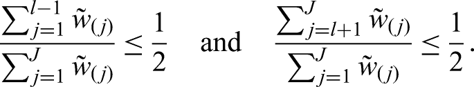
• The weighted median is selected as ${\tilde{p}}_{k,(l)}$ satisfying

  $$\frac{\sum _{j=1}^{l-1}{\tilde{w}}_{(j)}}{\sum _{j=1}^J{\tilde{w}}_{(j)}}\le \frac{1}{2}\mathrm{and}\frac{\sum _{j=l+1}^J{\tilde{w}}_{(j)}}{\sum _{j=1}^J{\tilde{w}}_{(j)}}\le \frac{1}{2}.$$

We adopt the weighted median because it is a more robust estimator compared with the weighted mean and the posterior mode may be ambiguous due to the multi-modal posterior distribution. More detailed discussions on $S(\cdot ,\cdot )$ with a numerical study are given in Section C of the Supplemental Appendix. The optimal dose for cohort $n+1$ based on the cumulative data up to cohort $n$ , $Y_n$ and $M_n$ , is defined as

$$d_{n+1}^{*}={\text{argmin}}_{k=1,\dots ,K}|{\hat{p}}_{n,k}-\varphi |.$$

2.3 Prior elicitation

While the ABC design is flexible with respect to the choice of the prior $\pi (p_1,\dots ,p_K)$ , the prior samples $\{p_{k,(j)}{\}}_{k=1}^K$ play an important role for efficiently identifying the MTD. To enhance the robustness of the ABC design, we should generate samples without any parametric dose–toxicity assumption, for which an intuitive way is to first generate $K$ samples from $\mathrm{Uniform}(0,1)$ and then sort them in an ascending order. However, this method does not take the target rate $\varphi$ into consideration and, as a result, the prior samples are less informative and lead to poor performance.

Before conducting a phase I trial, we are typically provided with the target toxicity rate $\varphi$ as well as the toxicity probability monotone constraint. Thus, it is desirable to encode both parts of information in the prior to obtain more informative samples. The main goal of the phase I design is to find the dose level $k$ whose DLT rate is closed to $\varphi$ . Because each dose could possibly be the MTD, we can generate prior samples of $p_1,\dots ,p_K$ from $K+1$ possible models $\{{\mathcal{M}}_k{\}}_{k=0}^K$ , where ${\mathcal{M}}_k$ is the model that dose level $k$ is the MTD while ${\mathcal{M}}_0$ indicates that all the dose levels are overly toxic (i.e. no MTD). This way of incorporating $\varphi$ into the model provides more informative prior samples for the ABC design.

Consequently, we propose to generate the prior samples as follows:

Considering the trade-off between computation and performance, we generate $20,000$ prior samples of $p_1,\dots ,p_K$ from each model ${\mathcal{M}}_k$ , which leads to a total number of $J=20,000\times (K+1)$ prior samples. The prior samples from $\pi (p_1,\dots ,p_K)$ are obtained from all $(K+1)$ models, $\{{\mathcal{M}}_k{\}}_{k=0}^K$ . These prior samples can be generated before the trial conduct and saved for repeated use.

Given ${\mathcal{M}}_k$ with $k\ne 0$ ,

Set dose level $k$ as the target with a DLT rate $p_{k,(j)}\sim \text{Uniform}(\varphi -\delta ,\varphi +\delta )$ where $\delta$ is a prespecified small number.

We independently generate $k-1$ samples from $\text{Uniform}(0,\varphi -\delta )$ and sort them in an ascending order to obtain $\{p_{1,(j)},\dots ,p_{k-1,(j)}\}$ .

We independently generate $K-k$ samples from $\text{Uniform}(\varphi +\delta ,2\varphi )$ and sort them in an ascending order to obtain $\{p_{k+1,(j)},\dots ,p_{K,(j)}\}$ .

Under ${\mathcal{M}}_0$ , we independently generate $K$ samples from $\text{Uniform}(\varphi +\delta ,2\varphi )$ and sort them in an ascending order to obtain $\{p_{1,(j)},\dots ,p_{K,(j)}\}$ .

The neighborhood parameter $\delta$ controls the distinguishability of the target dose level in the generated prior samples. A larger value of $\delta$ indicates that the MTD is easier to be determined in the prior samples, and vice versa. In Sensitivity Analysis Section, we conduct extensive simulation studies to show that the ABC design is not sensitive to the choice of $\delta$ , and we recommend $\delta =0.1$ as a default value in practice.

2.4 Dose-finding algorithm

To ensure the safety and benefit for the patients, we further impose an early stopping criterion in the ABC design. We terminate the trial when there is strong evidence indicating the lowest dose level is still overly toxic. We assign Jeffreys’ $\mathrm{Beta}(0.5,0.5)$ prior distribution to the DLT rate $p_1$ , and terminate the trial if $Pr(p_1>\varphi |y_1,m_1\ge 3)>0.95$ .

The dose-finding procedure of the ABC design is detailed as follows:

Treat the first cohort of patients at the lowest or the physician-specified dose level.

After enrolling $n$ cohorts, select the optimal dose level $d_{n+1}^{*}={\text{argmin}}_{k=1,\dots ,K}|{\hat{p}}_{n,k}-\varphi |$ based on (1).

According to the optimal dose level $d_{n+1}^{*}$ ,

If $d_n>d_{n+1}^{*}$ , then $d_{n+1}=d_n-1$ .

If $d_n=d_{n+1}^{*}$ , then $d_{n+1}=d_n$ .

If $d_n<d_{n+1}^{*}$ , then $d_{n+1}=d_n+1$ .

The trial can be either stopped after exhaustion of the maximum sample size, or be terminated early for safety if the lowest dose level is too toxic by the early stopping rule, $Pr(p_1>\varphi |y_1,m_1\ge 3)>0.95$ .

At the end of the trial, the observed data $(Y_N,M_N)$ are collected, where $N$ is the total number of cohorts. The MTD is then estimated with another round of ABC simulation, that is, $d^{*}$ is finally selected as

$$d^{*}={\text{argmin}}_{k=1,\dots ,K}|{\hat{p}}_{N,k}-\varphi |.$$

If the DLT rate of the recommended MTD must be lower than the target, we can easily make a modification by first identifying $d^{*}$ , while if $d^{*}$ is higher than the target then we simply choose the next lower dose as the MTD.

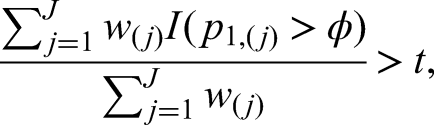
In the dose-finding algorithm, we adopt the same early termination rule as those in most of the interval designs^8,11 for a fair comparison. However, as our prior samples involve model ${\mathcal{M}}_0$ (i.e. all doses are overly toxic), it is possible to construct our own early termination rule as

$$\frac{\sum _{j=1}^J{w}_{(j)}I(p_{1,(j)}>\varphi )}{\sum _{j=1}^J{w}_{(j)}}>t,$$

where $t$ is the threshold value, for example, $t=0.95$ .

3 Simulation studies

3.1 Sensitivity analysis

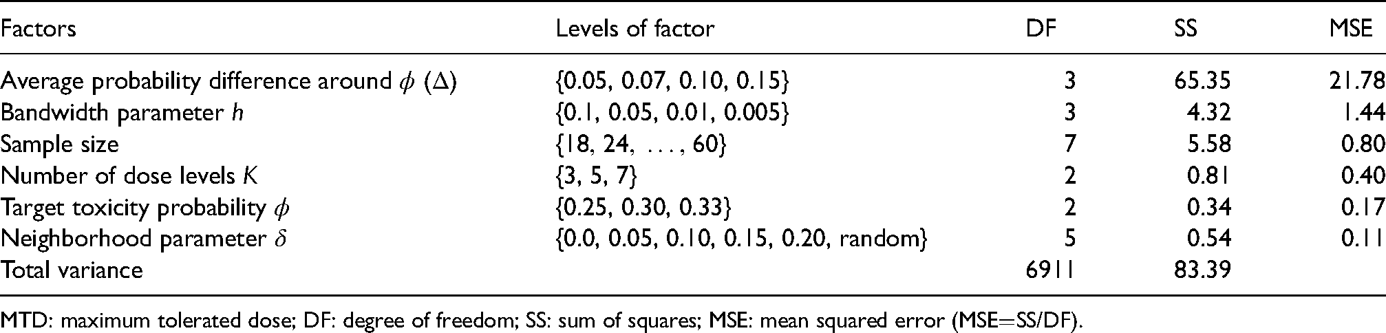
We investigate the effect of the parameters $\delta$ and $h$ on the performance of the ABC design with the analysis of variance (ANOVA) method. ²⁷ We randomly generate dose–toxicity scenarios following the procedure in Paoletti et al. ²⁸ as described in Section A.2 of the Supplemental Appendix. To conduct a comprehensive analysis with randomly generated scenarios, we consider four influential factors in phase I trials, including the average probability difference $\mathrm{\Delta }$ around the target, the number of dose levels $K$ , the sample size as well as the target toxicity rate $\varphi$ . The first three factors affect the difficulty of the MTD-identification task, where larger $\mathrm{\Delta }$ , smaller $K$ , and larger sample size would typically result in higher MTD selection percentages. The possible levels of the four factors are listed in Table 1, which yields $4\times 3\times 8\times 3=288$ different configurations. Under each configuration, we investigate the performance of the ABC design via $1000$ randomly generated scenarios when $\delta$ takes a value of $\{0,0.05,0.10,0.15,0.20\}$ or $\delta$ is randomly selected from Uniform $(0,0.2)$ and $h$ is selected from $\{0.1,0.05,0.01,0.005\}$ .

Table 1

The simulation factors that may affect the dose-finding performance of phase I trial design and the results of ANOVA in terms of the percentage of MTD selection. The ANOVA also includes all the pairwise interactions between the five simulation factors.

Factors	Levels of factor	DF	SS	MSE
Average probability difference around $\varphi$ ( $\mathrm{\Delta }$ )	{0.05, 0.07, 0.10, 0.15}	3	65.35	21.78
Bandwidth parameter $h$	{0.1, 0.05, 0.01, 0.005}	3	4.32	1.44
Sample size	$\{18,24,\dots ,60\}$	7	5.58	0.80
Number of dose levels $K$	{3, 5, 7}	2	0.81	0.40
Target toxicity probability $\varphi$	{0.25, 0.30, 0.33}	2	0.34	0.17
Neighborhood parameter $\delta$	{0.0, 0.05, 0.10, 0.15, 0.20, random}	5	0.54	0.11
Total variance		6911	83.39

MTD: maximum tolerated dose; DF: degree of freedom; SS: sum of squares; MSE: mean squared error (MSE $=$ SS/DF).

After obtaining the percentage of MTD selection under each configuration with different values of $(\delta ,h)$ , we perform ANOVA with regard to these percentages using the simulation factors including all the pairwise interactions in Table 1. In the ANOVA, we also regard the tuning parameters $\delta$ and $h$ as two additional factors in the evaluation of dose-finding performance. Thus, the degree of freedom of the total variance for ANOVA is $288\times 6\times 4-1=6911$ . Among the six influential factors, the neighborhood parameter $\delta$ has the least effect on the performance of the ABC design in terms of the mean squared error (MSE). In particular, $\delta$ only accounts for $0.64\text{\%}$ $(0.54/83.39)$ of the MTD selection percentage variance, which indicates the ABC design is robust to the choice of $\delta$ . The performance of the ABC design is more sensitive to the bandwidth parameter $h$ , because it is the second most influential factor on the MTD selection percentage.

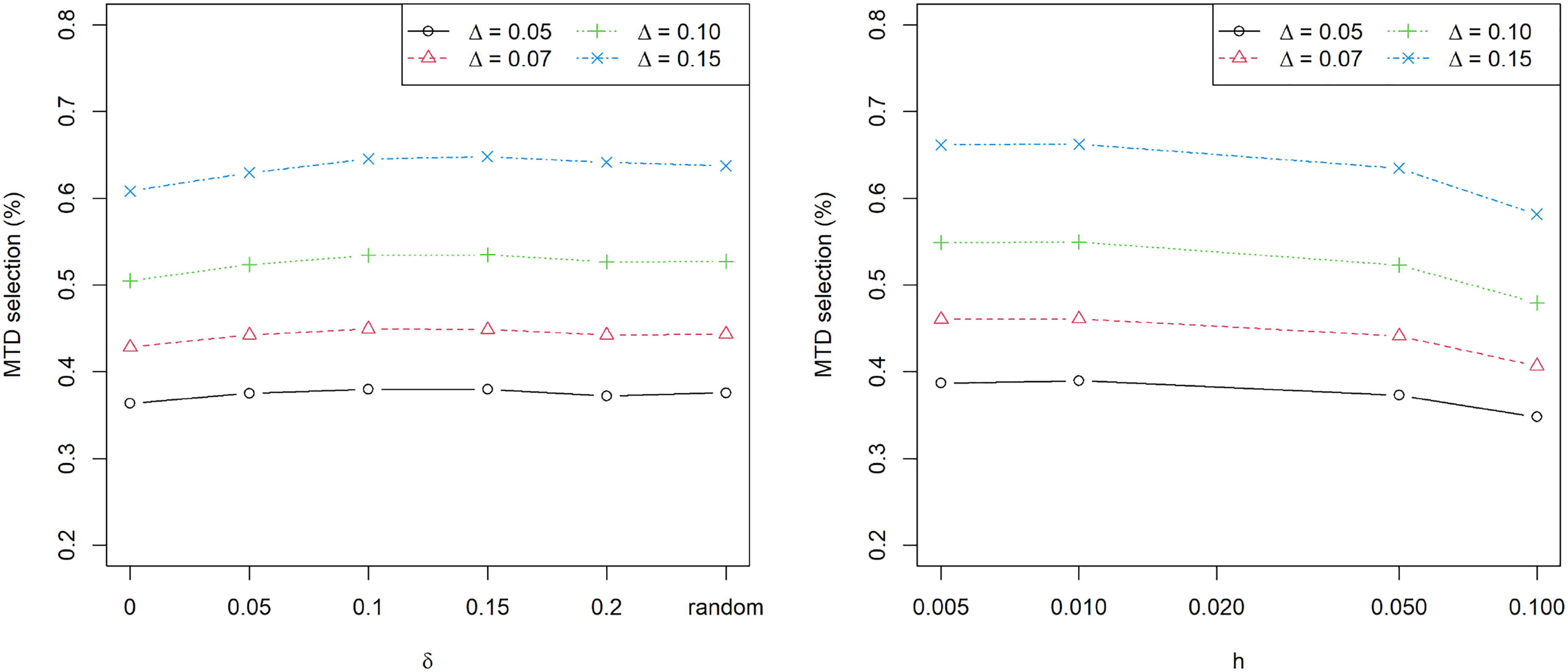
From Table 1, it is clear that the average probability difference $\mathrm{\Delta }$ around the target is the dominating factor for the percentage of MTD selection, as it contributes the largest MSE (significantly larger than the second) in the ANOVA. We further study the effect of the tuning parameters $\delta$ and $h$ on the MTD selection percentage under different values of $\mathrm{\Delta }$ . Figure 1 shows the MTD selection percentage versus the tuning parameters $\delta$ and $h$ for $\mathrm{\Delta }=\{0.05,0.07,0.10,0.15\}$ . Under various levels of trial difficulty (the difficulty of MTD identification decreases as $\mathrm{\Delta }$ increases), $\delta$ shows relatively minor effect on the performance of the ABC design, demonstrating the insensitivity of the design to $\delta \in [0.05,0.20]$ . As for the bandwidth parameter $h$ , it is clear that a larger value of $h$ would undermine the performance of the ABC design. When $h$ is decreased close to $0.01$ , the performance of the ABC design is saturated and further reduction of $h$ would not improve the trial performance. In practice, it is recommended to choose any value of $\delta \in [0.05,0.20]$ and $h=0.01$ for the ABC design, and by default we set $\delta =0.1$ and $h=0.01$ .

Figure 1

The maximum tolerated dose (MTD) selection percentage versus the neighborhood parameter $\delta$ (left) and bandwidth parameter $h$ (right) under the probability difference around the target $\mathrm{\Delta }=\{0.05,0.07,0.10,0.15\}$ . We set $\delta =\{0,0.05,0.1,0.15,0.2\}$ , respectively, and also consider the case of randomly choosing $\delta$ from Uniform $(0,0.2)$ and $h$ takes a value of $\{0.005,0.01,0.05,0.1\}$ .

3.2 Evaluation under random scenarios

To make an extensive comparison of the ABC design with existing methods, we select six state-of-the-art phase I designs, including the CRM design with the power model whose model skeleton is selected using the method of Lee and Cheung ²⁹ the CCD design ⁶ which is based on the Markov chain theory, the modified toxicity probability interval (mTPI) design, ⁷ the Bayesian optimal interval design (BOIN), ⁸ the keyboard design, ⁹ as well as the uniformly most powerful Bayesian interval (UMPBI) design. ¹¹ Among the six designs, the CRM is the only model-based one, while the other five are algorithm-based methods and, more specifically, they are all interval designs. Unless otherwise stated, all the six existing designs adopt the default parameters following the original papers and we utilize the same early stopping rule for the five interval designs and the ABC design, that is, if $Pr(p_1>\varphi |y_1,m_1\ge 3)>0.95$ , we terminate the trial for safety. For the early termination rule under the CRM, the posterior probability of $p_1>\varphi$ is calculated based on the CRM model and the threshold probability is still set at $0.95$ . The detailed settings for the six existing designs are given in Section A.1 of the Supplemental Appendix.

We investigate five dose levels for each trial and set the target toxicity rate $\varphi =0.3$ and $0.2$ , respectively. The sample size is $30$ and patients are treated in a cohort size of $3$ . To avoid cherry-picking, we randomly generate dose–toxicity scenarios following the procedure in Paoletti et al., ²⁸ which is detailed in Section A.2 of the Supplemental Appendix. The average probability difference $\mathrm{\Delta }$ around the target is controlled at $0.05$ , $0.07$ , $0.1$ and $0.15$ , respectively, and under each value of $\mathrm{\Delta }$ , we replicate $5000$ simulations.

Four summary statistics are adopted to evaluate the performances of the seven designs under comparison. The two main measurements, reflecting the accuracy and efficiency of a design, are the percentage of MTD selection and the percentage of patients treated at the MTD (MTD allocation), for which larger values are preferred. The remaining two measurements quantify the safety aspects of a trial, including the percentage of trials that select overdoses as the MTD (overdose selection), and the percentage of patients allocated to overdoses (overdose allocation). A design with smaller values of the two safety statistics would be considered more ethical and desirable. To quantify the variability, we adopt the bootstrap method to construct the 95% confidence intervals for each measurement, that is, we resample $5000$ trial results with replacement from a total of $5000$ repetitions (random scenarios) and repeat the resampling procedure for $1000$ times to obtain the confidence intervals.

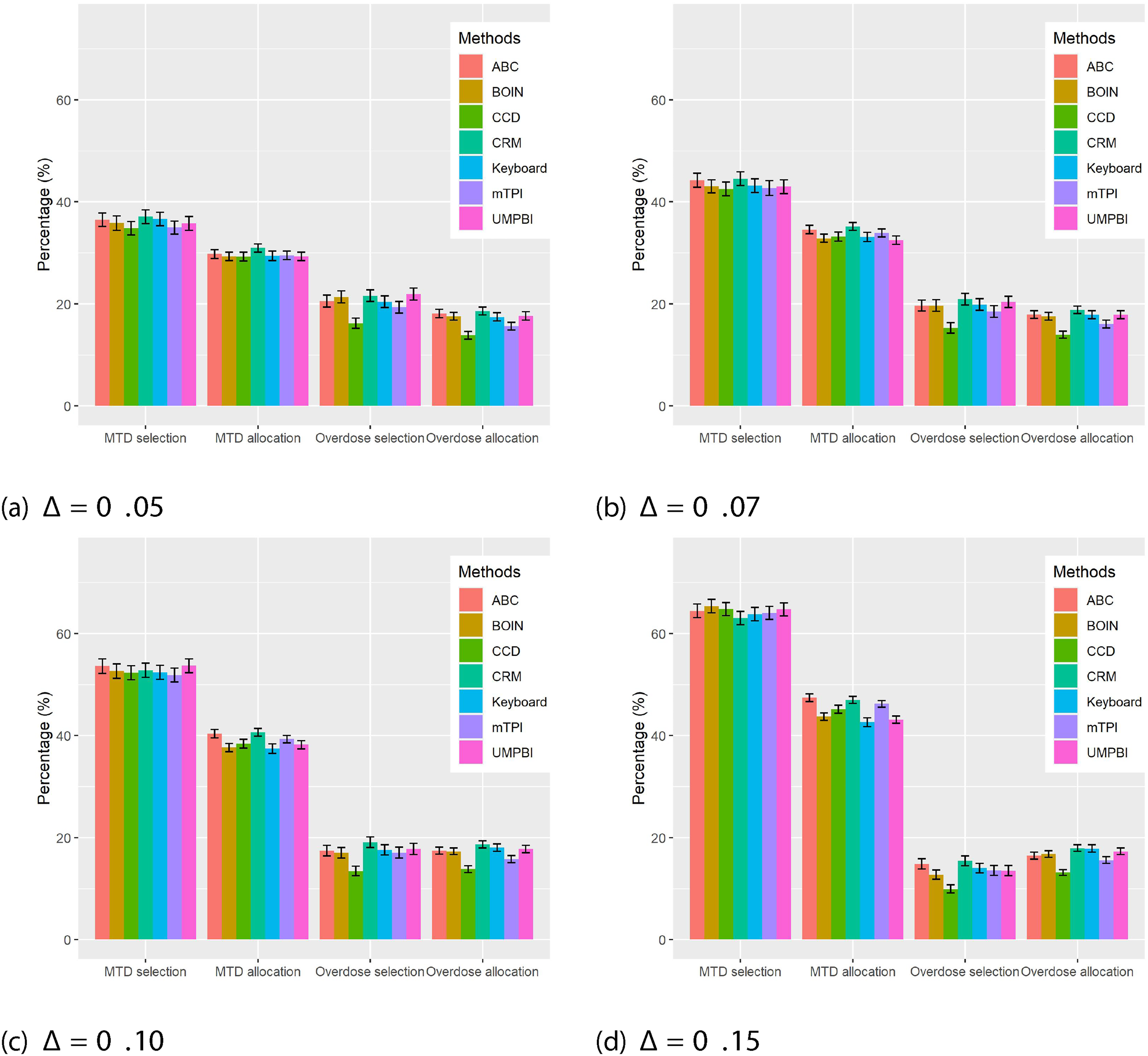
The results with $\varphi =0.3$ are shown in Figure 2. The performances of all the designs improve as $\mathrm{\Delta }$ increases. The efficiency of using all the available data under the ABC and CRM designs is reflected by the MTD allocation metric, for which both designs yield higher MTD allocation percentages compared with the other interval designs. The gap becomes more significant when $\mathrm{\Delta }$ increases. In terms of the MTD selection percentage, both the ABC and CRM designs are superior to the interval designs when $\mathrm{\Delta }$ is small; the gap diminishes when $\mathrm{\Delta }$ becomes large. When $\mathrm{\Delta }$ is large, the information from the MTD neighborhood data may be adequate to identify the MTD well, and thus using all the available data does not boost the performance greatly. Under the setting of $\mathrm{\Delta }=0.15$ , BOIN performs best, while CRM yields the lowest MTD selection percentage compared with the counterparts. The performances of the ABC design are robust across all different values of $\mathrm{\Delta }$ , which reveals the advantage of imposing no dose–toxicity assumption in ABC.

Figure 2

Simulation results with sample size $30$ based on 5000 randomly generated dose–toxicity scenarios under the average probability difference of $\mathrm{\Delta }=0.05$ , 0.07, 0.10 and 0.15 around the target toxicity probability $\varphi =0.30$ , respectively. The error bar represents the 95% confidence interval for each measurement.

With regard to the two safety measurements, the CRM has the highest percentages of overdose selection and overdose allocation among the seven designs. The CCD design performs best in terms of the safety metrics, while its performances are worse for the two accuracy measurements. The other five designs are comparable in terms of the safety metrics.

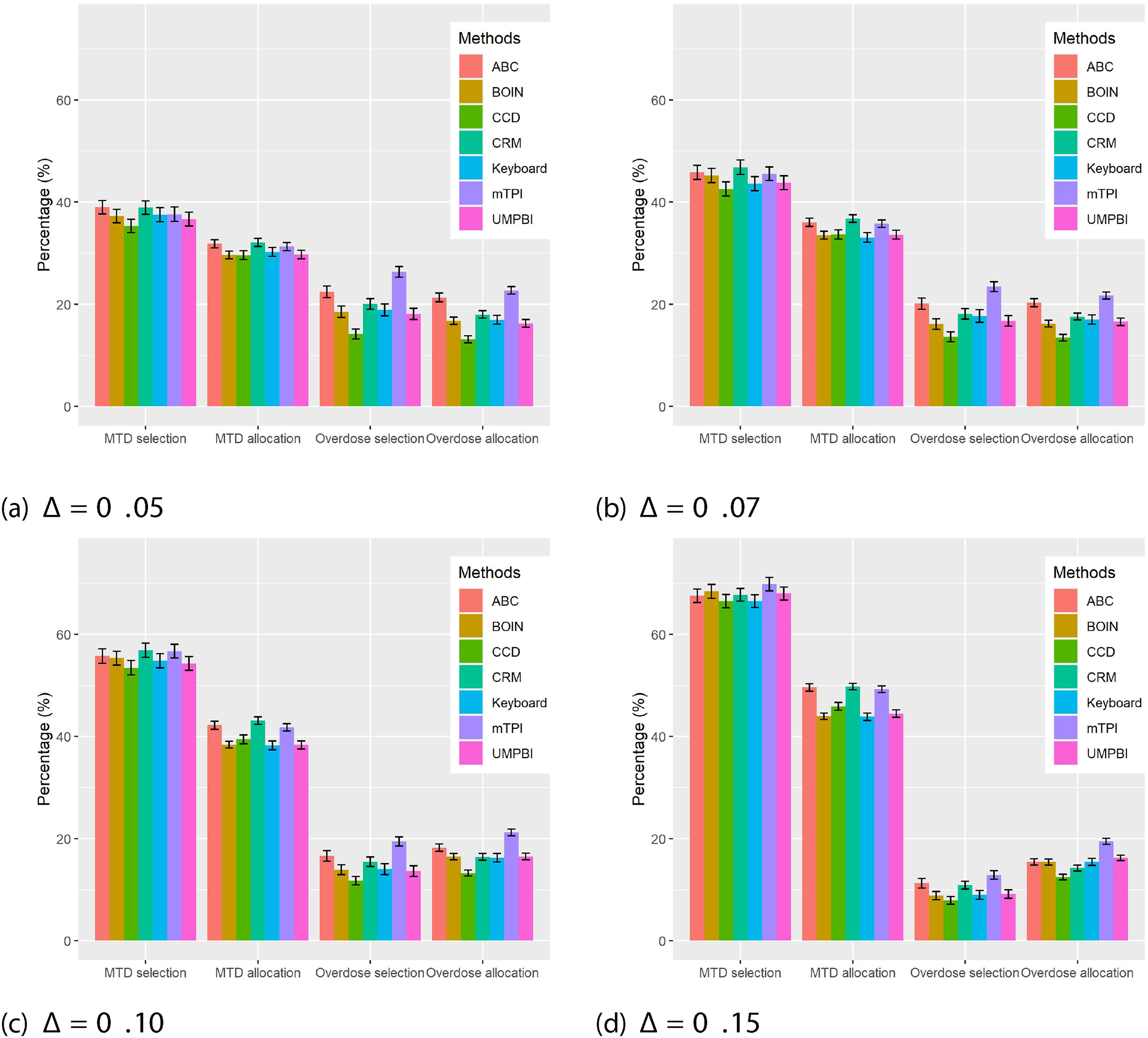
The results with $\varphi =0.2$ are presented in Figure 3. Overall, the performances of the seven designs are similar to those under the settings of $\varphi =0.3$ . However, when $\varphi =0.2$ , the mTPI design appears to be very aggressive. The mTPI yields similar performances to the ABC and CRM designs in terms of the MTD selection and allocation metrics, while it sacrifices safety significantly in contrast with other methods. In summary, numerical comparisons with the six well-known methods demonstrate the robustness and efficiency of the ABC design.

Figure 3

Simulation results with sample size $30$ based on 5000 randomly generated dose–toxicity scenarios under the average probability difference of $\mathrm{\Delta }=0.05$ , 0.07, 0.10 and 0.15 around the target toxicity probability $\varphi =0.20$ , respectively. The error bar represents the 95% confidence interval for each measurement.

3.3 Evaluation under fixed scenarios

To gain more insight into the ABC design, we evaluate its performance under five representative fixed scenarios. For an objective comparison with no cherry-picking, we adopt the fixed scenarios in Table 1 of Cheung and Chappell. ¹⁴ The number of dose levels is $K=6$ and the target toxicity rate is $\varphi =0.2$ . The comparisons are again made with the six phase I designs under the similar settings as introduced in Section A.1 of the Supplemental Appendix. The total sample size is $36$ and patients are treated with a cohort size of $3$ . We use the same early stopping rules as those under the random scenarios. Under each scenario, we replicate 5000 simulations.

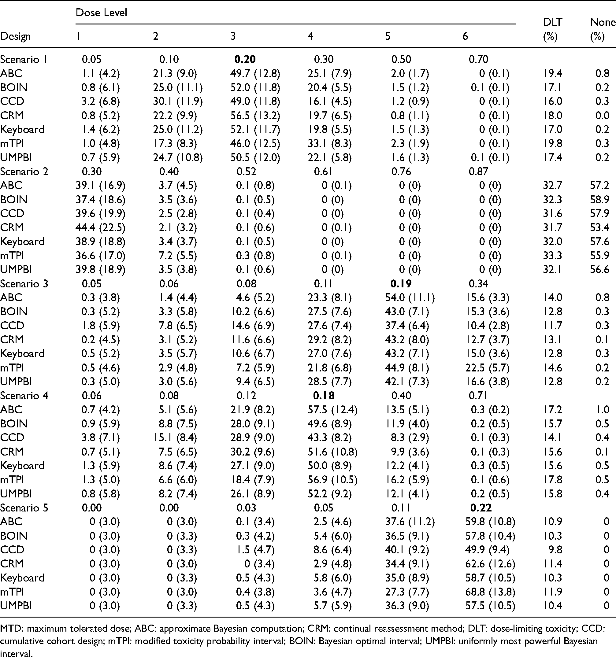
The detailed information and results under the fixed scenarios are summarized in Table 2. Under scenario 1, the CRM has the best performance, while the other designs yield comparable results. In scenario 2, all the dose levels are overly toxic, and the ABC design and all interval designs show satisfactory and comparable results by early stopping the trials, but the CRM yields a slightly lower non-selection percentage ( $53.4\text{\%}$ ) compared with others. The ABC design leads to the best performance under both scenarios 3 and 4 and the gaps of MTD selection percentages are around $10\text{\%}$ under scenario 3. Under scenario 5 where the last dose level is the MTD, the mTPI design is substantially better than others, while it tends to select over-toxic dose level as the MTD as shown in scenarios 1, 3, and 4. Except for the mTPI design, the ABC design has slightly higher over-dose selection percentages under scenarios 1, 3, and 4, while the gaps are marginal. Overall, the ABC design yields satisfactory performances for all of the five fixed scenarios.

Table 2

The percentages of MTD selection (the numbers of patients treated at each dose) under the ABC design in comparison with the BOIN, CCD, CRM, Keyboard, mTPI and UMPBI designs under six fixed scenarios with the target toxicity probability 0.20 in boldface when sample size is $36$ . None represents the percentage of trials of non-selection due to early stopping.

	Dose Level						DLT	None
Design	1	2	3	4	5	6	(%)	(%)
Scenario 1	0.05	0.10	0.20	0.30	0.50	0.70
ABC	1.1 (4.2)	21.3 (9.0)	49.7 (12.8)	25.1 (7.9)	2.0 (1.7)	0 (0.1)	19.4	0.8
BOIN	0.8 (6.1)	25.0 (11.1)	52.0 (11.8)	20.4 (5.5)	1.5 (1.2)	0.1 (0.1)	17.1	0.2
CCD	3.2 (6.8)	30.1 (11.9)	49.0 (11.8)	16.1 (4.5)	1.2 (0.9)	0 (0.1)	16.0	0.3
CRM	0.8 (5.2)	22.2 (9.9)	56.5 (13.2)	19.7 (6.5)	0.8 (1.1)	0 (0.1)	18.0	0.0
Keyboard	1.4 (6.2)	25.0 (11.2)	52.1 (11.7)	19.8 (5.5)	1.5 (1.3)	0 (0.1)	17.0	0.2
mTPI	1.0 (4.8)	17.3 (8.3)	46.0 (12.5)	33.1 (8.3)	2.3 (1.9)	0 (0.1)	19.8	0.3
UMPBI	0.7 (5.9)	24.7 (10.8)	50.5 (12.0)	22.1 (5.8)	1.6 (1.3)	0.1 (0.1)	17.4	0.2
Scenario 2	0.30	0.40	0.52	0.61	0.76	0.87
ABC	39.1 (16.9)	3.7 (4.5)	0.1 (0.8)	0 (0.1)	0 (0)	0 (0)	32.7	57.2
BOIN	37.4 (18.6)	3.5 (3.6)	0.1 (0.5)	0 (0)	0 (0)	0 (0)	32.3	58.9
CCD	39.6 (19.9)	2.5 (2.8)	0.1 (0.4)	0 (0)	0 (0)	0 (0)	31.6	57.9
CRM	44.4 (22.5)	2.1 (3.2)	0.1 (0.6)	0 (0.1)	0 (0)	0 (0)	31.7	53.4
Keyboard	38.9 (18.8)	3.4 (3.7)	0.1 (0.5)	0 (0)	0 (0)	0 (0)	32.0	57.6
mTPI	36.6 (17.0)	7.2 (5.5)	0.3 (0.8)	0 (0.1)	0 (0)	0 (0)	33.3	55.9
UMPBI	39.8 (18.9)	3.5 (3.8)	0.1 (0.6)	0 (0)	0 (0)	0 (0)	32.1	56.6
Scenario 3	0.05	0.06	0.08	0.11	0.19	0.34
ABC	0.3 (3.8)	1.4 (4.4)	4.6 (5.2)	23.3 (8.1)	54.0 (11.1)	15.6 (3.3)	14.0	0.8
BOIN	0.3 (5.2)	3.3 (5.8)	10.2 (6.6)	27.5 (7.6)	43.0 (7.1)	15.3 (3.6)	12.8	0.3
CCD	1.8 (5.9)	7.8 (6.5)	14.6 (6.9)	27.6 (7.4)	37.4 (6.4)	10.4 (2.8)	11.7	0.3
CRM	0.2 (4.5)	3.1 (5.2)	11.6 (6.6)	29.2 (8.2)	43.2 (8.0)	12.7 (3.7)	13.1	0.1
Keyboard	0.5 (5.2)	3.5 (5.7)	10.6 (6.7)	27.0 (7.6)	43.2 (7.1)	15.0 (3.6)	12.8	0.3
mTPI	0.5 (4.6)	2.9 (4.8)	7.2 (5.9)	21.8 (6.8)	44.9 (8.1)	22.5 (5.7)	14.6	0.2
UMPBI	0.3 (5.0)	3.0 (5.6)	9.4 (6.5)	28.5 (7.7)	42.1 (7.3)	16.6 (3.8)	12.8	0.2
Scenario 4	0.06	0.08	0.12	0.18	0.40	0.71
ABC	0.7 (4.2)	5.1 (5.6)	21.9 (8.2)	57.5 (12.4)	13.5 (5.1)	0.3 (0.2)	17.2	1.0
BOIN	0.9 (5.9)	8.8 (7.5)	28.0 (9.1)	49.6 (8.9)	11.9 (4.0)	0.2 (0.5)	15.7	0.5
CCD	3.8 (7.1)	15.1 (8.4)	28.9 (9.0)	43.3 (8.2)	8.3 (2.9)	0.1 (0.3)	14.1	0.4
CRM	0.7 (5.1)	7.5 (6.5)	30.2 (9.6)	51.6 (10.8)	9.9 (3.6)	0.1 (0.3)	15.6	0.1
Keyboard	1.3 (5.9)	8.6 (7.4)	27.1 (9.0)	50.0 (8.9)	12.2 (4.1)	0.3 (0.5)	15.6	0.5
mTPI	1.3 (5.0)	6.6 (6.0)	18.4 (7.9)	56.9 (10.5)	16.2 (5.9)	0.1 (0.6)	17.8	0.5
UMPBI	0.8 (5.8)	8.2 (7.4)	26.1 (8.9)	52.2 (9.2)	12.1 (4.1)	0.2 (0.5)	15.8	0.4
Scenario 5	0.00	0.00	0.03	0.05	0.11	0.22
ABC	0 (3.0)	0 (3.0)	0.1 (3.4)	2.5 (4.6)	37.6 (11.2)	59.8 (10.8)	10.9	0
BOIN	0 (3.0)	0 (3.3)	0.3 (4.2)	5.4 (6.0)	36.5 (9.1)	57.8 (10.4)	10.3	0
CCD	0 (3.0)	0 (3.3)	1.5 (4.7)	8.6 (6.4)	40.1 (9.2)	49.9 (9.4)	9.8	0
CRM	0 (3.0)	0 (3.0)	0 (3.4)	2.9 (4.8)	34.4 (9.1)	62.6 (12.6)	11.4	0
Keyboard	0 (3.0)	0 (3.3)	0.5 (4.3)	5.8 (6.0)	35.0 (8.9)	58.7 (10.5)	10.3	0
mTPI	0 (3.0)	0 (3.0)	0.4 (3.8)	3.6 (4.7)	27.3 (7.7)	68.8 (13.8)	11.9	0
UMPBI	0 (3.0)	0 (3.3)	0.5 (4.3)	5.7 (5.9)	36.3 (9.0)	57.5 (10.5)	10.4	0

MTD: maximum tolerated dose; ABC: approximate Bayesian computation; CRM: continual reassessment method; DLT: dose-limiting toxicity; CCD: cumulative cohort design; mTPI: modified toxicity probability interval; BOIN: Bayesian optimal interval; UMPBI: uniformly most powerful Bayesian interval.

4 Real trial application

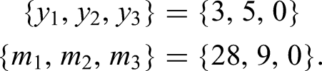
As an illustration, we apply the ABC design to the aforementioned phase I trial on the MEK inhibitor selumetinib in children with progressive LGG. The DLT outcomes were defined as any grade 4 toxicity (except lymphopenia), grade 3 neutropenia with fever, grade 3 thrombocytopenia with bleeding, any grade 3 or 4 toxicity possibly related to selumetinib, or any grade 2 toxicity persisting $\ge 7$ days that was medically significant or intolerable enough to interrupt or reduce the dose. Originally, the trial evaluated $37$ patients to estimate the MTD with the target toxicity rate $\varphi =0.25$ . Patients were assigned in a cohort size of $3$ to one of the three dose levels of the MEK inhibitor selumetinib $\{25,33,43\}$ mg/m ${}^2$ /dose bis in die via the CRM design based on the two-parameter logistic model. The observed data at dose levels 1–3 from the original clinical trial were

$$\begin{array}{rl}\{y_1,y_2,y_3\}& =\{3,4,2\}\\ \{m_1,m_2,m_3\}& =\{24,10,3\}.\end{array}$$

Based on the observed data in the trial, the estimated DLT rates were $\{0.125,0.400,0.667\}$ , and the MTD selected using the CRM method was dose level 1. ²³

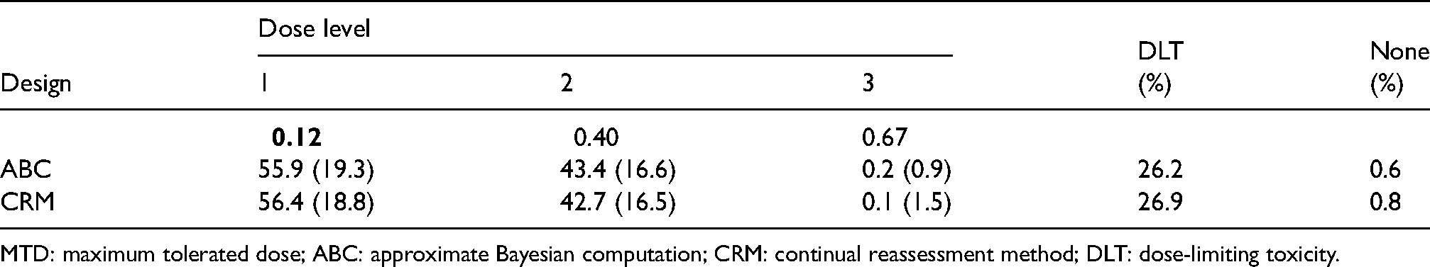
We applied the ABC design with $\delta =0.1$ and $h=0.01$ to this trial based on the estimated DLT rates. There were 13 cohorts in total where the last cohort contained only one subject. For comparison, we also include the CRM design using the two-parameter logistic model, for which the detail is given in Section A.1 of the Supplemental Appendix. The entire procedure is repeated for $5000$ times and the results are presented in Table 3. It is clear that the ABC design yields comparable performances to the CRM design under this trial example. Nevertheless, the ABC design is model-free, and thus it is more robust and easier to use in practice.

Table 3

The percentages of MTD selection (the numbers of patients treated at each dose) under the ABC and CRM designs with 5000 replications. The target toxicity probability is 0.25 in the real trial application with 37 patients.

Design	Dose level			DLT	None
	1	2	3	(%)	(%)
	0.12	0.40	0.67
ABC	55.9 (19.3)	43.4 (16.6)	0.2 (0.9)	26.2	0.6
CRM	56.4 (18.8)	42.7 (16.5)	0.1 (1.5)	26.9	0.8

MTD: maximum tolerated dose; ABC: approximate Bayesian computation; CRM: continual reassessment method; DLT: dose-limiting toxicity.

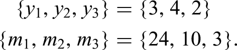
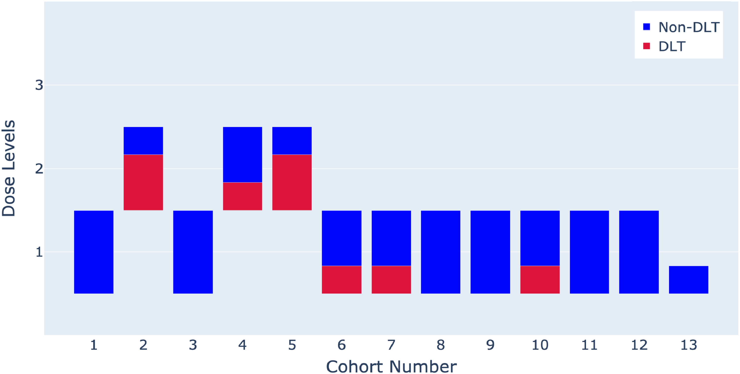
To better demonstrate the property of the ABC design, we present the detailed trial flow of one specific trial selected from the $5000$ repetitions. The patient allocations and outcomes are shown in Figure 4. The trial started by treating the first cohort of patients at the lowest dose level. In the first cohort, there was no DLT observed, which yielded the estimated DLT rates $\{{\hat{p}}_{1,k}{\}}_{k=1}^3=(0.08,0.22,0.40)$ . Thus, the trial decided to escalate to dose level 2 for the second cohort, where we observed two DLTs among three patients, resulting in the estimated DLT rates $\{{\hat{p}}_{2,k}{\}}_{k=1}^3=(0.18,0.37,0.45)$ . Consequently, the next cohort was assigned back to dose level 1, where again no patient experienced the DLT, leading to $\{{\hat{p}}_{3,k}{\}}_{k=1}^K=(0.12,0.33,0.44)$ . Consequently, the trial escalated to dose level 2 for cohort 4 and one out of the three patients experienced the DLT, which led to $\{{\hat{p}}_{4,k}{\}}_{k=1}^K=(0.11,0.33,0.44)$ . As a result, the trial remained at dose level 2 for the next cohort, but two DLT outcomes were observed among the three patients and thus the trial de-escalated back to dose level 1. All the remaining cohorts were assigned to dose level 1. Finally, the observed data at dose levels 1–3 were

$$\begin{array}{rl}\{y_1,y_2,y_3\}& =\{3,5,0\}\\ \{m_1,m_2,m_3\}& =\{28,9,0\}.\end{array}$$

Upon the completion of the trial, we selected dose level 1 (i.e. the dose of 25  mg/m ${}^2$ /dose bis in die) as the MTD, which is consistent with the original selection by the CRM design. ²³

Figure 4

Patient allocations and outcomes by the ABC design for the real trial illustration using a representative trial among the $5000$ repetitions. The ABC recommended MTD is dose level 1. MTD: maximum tolerated dose; ABC: approximate Bayesian computation.

5 Conclusion

We have proposed a new phase I design for identifying the MTD using the approximate Bayesian computation method. The ABC design possesses the merits of both model-free and model-based designs simultaneously. Because it is model-free, there is no need to impose any assumption on the dose–toxicity curve, which avoids the risk of model misspecification. Similar to the model-based methods, the ABC design is also efficient by aggregating all the available information when deciding dose assignment for each new cohort. As demonstrated by simulation studies, the ABC design performs well in terms of both the efficiency and robustness in phase I trials. Compared with other phase I designs, the ABC design shows advantages in terms of the MTD selection and patient allocation under the random scenarios. There are two tuning parameters $\delta$ and $h$ in the ABC design. The neighborhood parameter $\delta$ has rather minor effect on the design performance, as shown by the comprehensive simulation studies and ANOVA in Sensitivity Analysis Section, while the bandwidth parameter $h$ can be simply fixed at $h=0.01$ to achieve satisfactory performance. In practice, the ABC design is easy to use, because there is no need to carry out the extensive parameter calibration prior to the trial conduct. Therefore, the ABC design can be broadly used in phase I clinical trials due to its robust and efficient properties as well as the ease of implementation. Under some cases in the simulation studies, our design shows a slightly higher but acceptable overdose selection percentage compared with existing phase I designs as a sacrifice for higher MTD selection and MTD allocation percentages. This is a trade-off often encountered in dose finding: by exploring more doses, it would help to pin down the MTD more accurately, while at the same time more patients might be put at the risk of exploring untried (higher) dose levels. The ABC design does not allow inserting some intermediate dose level during the trial, because a dose–toxicity model is typically needed for such dose insertion. Nevertheless, one possibility along this direction is to incorporate a working model to pin down the MTD more precisely through interpolation and dose insertion.

By incorporating the ABC sampling, our design can be easily extended to other more complicated phase I trials. To account for late-onset outcomes, the ABC design can be combined with the fractional scheme ³⁰ in a straightforward way. The only modification is to tune the bandwidth parameter $h$ under the late-onset context. To accommodate the efficacy outcomes, we can introduce the admissible set $\mathcal{A}$ and use a beta-binomial model to estimate the efficacy rates and thus deliver decisions through a trade-off between toxicity and efficacy. The ABC design can also be extended to the dose combination trials with an adaptation on generating prior samples, which warrants further investigation.

The implementation of the ABC design is simple and fast due to the fact that the prior samples can be generated beforehand. An application of our ABC design for dose finding (https://github.com/JINhuaqing/ABC) has been developed, where users can set various customized configurations for their trials and obtain visualization results of the ABC design. The R scripts for simulation studies as well as the real data application are available at https://github.com/JINhuaqing/ABC-simu.

Supplemental Material

sj-pdf-1-smm-10.1177_09622802221122402 - Supplemental material for Approximate Bayesian computation design for phase I clinical trials

Supplemental material, sj-pdf-1-smm-10.1177_09622802221122402 for Approximate Bayesian computation design for phase I clinical trials by Huaqing Jin, Wenbin Du and Guosheng Yin in Statistical Methods in Medical Research