Combined statistical decision limits based on two GH-2000 scores for the detection of growth hormone misuse

Abstract

The growth hormone-2000 biomarker method, based on the measurements of insulin-like growth factor-I and the amino-terminal pro-peptide of type III collagen, has been developed as a powerful technique for the detection of growth hormone misuse by athletes. Insulin-like growth factor-I and amino-terminal pro-peptide of type III collagen are combined in gender-specific formulas to create the growth hormone-2000 score, which is used to determine whether growth hormone has been administered. To comply with World Anti-Doping Agency regulations, each analyte must be measured by two methods. Insulin-like growth factor-I and amino-terminal pro-peptide of type III collagen can be measured by a number of approved methods, each leading to its own growth hormone-2000 score. Single decision limits for each growth hormone-2000 score have been introduced and developed by Bassett, Erotokritou-Mulligan, Holt, Böhning and their co-authors in a series of papers. These have been incorporated into the guidelines of the World Anti-Doping Agency. A joint decision limit was constructed based on the sample correlation between the two growth hormone-2000 scores generated from an available sample to increase the sensitivity of the biomarker method. This paper takes this idea further into a fully developed statistical approach. It constructs combined decision limits when two growth hormone-2000 scores from different assay combinations are used to decide whether an athlete has been misusing growth hormone. The combined decision limits are directly related to tolerance regions and constructed using a Bayesian approach. It is also shown to have highly satisfactory frequentist properties. The new approach meets the required false-positive rate with a pre-specified level of certainty.

1 Introduction

As a powerful anabolic agent of considerable therapeutic value, growth hormone (GH) is misused in sport to enhance performance. ¹ To preserve the fairness of competition, its use is prohibited by the World Anti-Doping Agency (WADA).^2–5 Two methods for the detection of GH misuse are currently available and approved by WADA: the isoform test developed by Bidlingmaier et al. ⁶ (see also WADA^2,3) and the GH-2000 biomarker test developed by the GH-2000 and GH-2004 projects. ⁷ The latter method depends on the measurements of two GH sensitive biomarkers, the insulin-like growth factor-I (IGF-I) and the amino-terminal pro-peptide of type III collagen (P-III-NP), both of which rise in response to exogenous GH administration.^8,9 The measured concentrations of the two biomarkers are combined in sex-specific and age-adjusted discriminant functions^10,11,7,12 to allow the calculation of a score, the GH-2000 score. It is possible that the score may take a negative value.

The measurements of IGF-I and P-III-NP are carried out by choosing two specific assays. As the measured results differ slightly from one assay to another, each assay pair generates an assay-specific GH-2000 score, which differs from other GH-2000 scores generated by different assays. These are the basis of the data generating process. Currently, there are three IGF-I assays and two P-III-NP assays approved by WADA. The IGF-I assays are a mass spectrometry (MS)-based approach, Immunotech A15729 IGF-I IRMA (Immunotech SAS, Marseille, France), and Immunodiagnostic Systems iSYS IGF-I (Immunodiagnostics Systems Limited, Boldon, UK). The P-III-NP assays are UniQ ${}^{\text{TM}}$ P-III-NP RIA (Orion Diagnostica, Espoo, Finland) and Siemens ADVIA Centaur P-III-NP (Siemens Healthcare Laboratory Diagnostics, Camberley, UK). For more details and background on these assays, see Holt et al. ⁷ As any GH-2000 score requires a pair of IGF-I assay and P-III-NP assay, there are six possible GH-2000 scores. Depending on the available technology, laboratories choose the appropriate GH-2000 scores for evaluating their samples, and a decision limit based on one single GH-2000 score has been developed in Holt et al. ⁷ and Böhning et al. ¹³ by assuming that a GH-2000 score from an athlete without GH misuse has a normal distribution.

As stated in Holt et al., ⁷ a result will be declared as an adverse analytical finding (i.e. indicative of doping) only if the confirmation procedure results in GH-2000 scores greater than the decision limits for two pairs of analytes. These decision limits are constructed on the basis of the univariate normal distributions of the associated GH-2000 scores. Erotokritou-Mulligan et al. ¹¹ with further details in Holt et al., ⁷ construct combined decision limits on the basis of a bivariate normal distribution. The idea is motivated by the intuition that a reduced correlation between the two GH-2000 scores could lead to reduced decision limits, and thus increase the sensitivity of GH misuse detection. We describe details of this method in Section 3.3.

The purpose of this paper is to provide a valid construction method of combined decision limits when two GH-2000 scores, based on two different pairs of IGF-I and P-III-NP assays, are used jointly in assessing the compliance of a sample. It is shown here how the combined decision limits are directly related to a particular tolerance region, and can be constructed so that the false positive rate (FPR) is controlled at a pre-specified level $1-\beta$ , say 1 in 10,000, with a pre-specified confidence or belief $1-\alpha$ , for example, $95\text{\%}$ , about the possible value of $(\mathit{\mu },\mathrm{\Sigma })$ , assuming the two GH-2000 scores have a bivariate normal distribution $N_2(\mathit{\mu },\mathrm{\Sigma })$ . This is in contrast to the previously mentioned method discussed in Erotokritou-Mulligan et al., ¹¹ where such a property is assumed to hold bona fide.

A Bayesian approach is adopted in this paper since a frequentist solution is much harder to construct and not available thus far (see Section 3.2 for more details). The frequentist property of the Bayesian combined decision limits is also assessed by simulation, which shows that the Bayesian combined decision limits can also be interpreted as frequentist combined decision limits.

The paper is organized as follows. Section 2 collects some known distributional results that will be used in Section 3. Section 3 considers the construction of decision limits. A very brief review of the construction of a single decision limit for one GH-2000 score is given in Section 3.1. Section 3.2 constructs Bayesian combined decision limits for two GH-2000 scores. The method is then illustrated with a real data set in Section 3.3. A simulation study is presented in Section 3.4 to assess the frequentist property of the Bayesian combined decision limits given in Section 3.3. Finally, the paper closes with a brief discussion in Section 4.

2 Preliminary distributional results

In this section, we collect some known distributional results, which are used in Section 3 for the construction of decision limits. More details about these results can be found in Guttman, ¹⁴ Box and Tao ¹⁵ and Anderson. ¹⁶

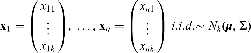
Following Holt et al. ⁷ and Böhning et al., ¹³ we assume that the GH-2000 scores $\mathbf{x}=(x_1,\dots ,x_k{)}^{\mathrm{\prime }}$ from an athlete without GH misuse have a $k$ -variate normal distribution $N_k(\mathit{\mu },\mathrm{\Sigma })$ , with both $\mathit{\mu }$ and $\mathrm{\Sigma }$ unknown. For the problem considered in this paper, we are only interested in the case of $k=2$ since only two GH-2000 scores are involved.We assume further that we have observed a random sample from the population $N_k(\mathit{\mu },\mathrm{\Sigma })$ :

$${\mathbf{x}}_1=\left(\begin{array}{c}{x}_{11}\\ ⋮\\ x_{1k}\end{array}\right),\dots ,{\mathbf{x}}_n=\left(\begin{array}{c}{x}_{n1}\\ ⋮\\ x_{nk}\end{array}\right)\stackrel{i.i.d.}{\sim }{N}_k(\mathit{\mu },\mathrm{\Sigma })$$

Denote $\mathbf{X}=({\mathbf{x}}_1,\dots ,{\mathbf{x}}_n)$ , $\overline{\mathbf{x}}=\sum _{i=1}^n{\mathbf{x}}_i/n$ , and $V=\sum _{i=1}^n({\mathbf{x}}_i-\overline{\mathbf{x}})({\mathbf{x}}_i-\overline{\mathbf{x}}{)}^{\prime }/(n-1)$ .

In this paper, the non-informative reference prior distribution of $(\mathit{\mu },{\mathrm{\Sigma }}^{-1})$ given by

$$p(\mathit{\mu },{\mathrm{\Sigma }}^{-1})\propto p(\mathit{\mu })P({\mathrm{\Sigma }}^{-1})\propto |{\mathrm{\Sigma }}^{-1}{|}^{-(k+1)/2}$$

(1)is used since the sample $\mathbf{X}$ is all we have. An additional incentive for using the non-informative reference prior is that the Bayesian decision limit for the special case of $k=1$ is also the frequentist decision limit; see Section 3.1 below.

The posterior distribution of $(\mathit{\mu },{\mathrm{\Sigma }}^{-1})$ based on the observed data $\mathbf{X}$ is then given by

$$p(\mathit{\mu },{\mathrm{\Sigma }}^{-1}|\mathbf{X})\propto |{\mathrm{\Sigma }}^{-1}{|}^{(n-k-1)/2}\exp \{-\frac{1}{2}tr{\mathrm{\Sigma }}^{-1}[(n-1)V+n(\mathit{\mu }-\overline{\mathrm{x}})(\mathit{\mu }-\overline{\mathbf{x}}{)}^{\prime }]\}$$

where $trA$ denotes the trace of matrix $A$ . Integrating out $\mathit{\mu }$ gives the posterior distribution of ${\mathrm{\Sigma }}^{-1}$

$${\mathrm{\Sigma }}^{-1}|\mathbf{X}\sim W_k([(n-1)V{]}^{-1},n-k)$$

(2)in the notation of Box and Tao, ¹⁵ and the posterior conditional (on ${\mathrm{\Sigma }}^{-1}$ ) distribution of $\mathit{\mu }$ is

$$p(\mathit{\mu }|{\mathrm{\Sigma }}^{-1},\mathbf{X})=\frac{p(\mu \mathit{,}{\mathrm{\Sigma }}^{-1}|\mathbf{X})}{\mathrm{p}({\mathrm{\Sigma }}^{-1}|\mathbf{X})}\sim N_k(\overline{\mathbf{x}},\mathrm{\Sigma }/n)$$

(3)

3 Decision limits

In this section, we consider the construction of decision limits. In Sction 3.1, we provide a very brief review of the construction of decision limit for one single GH-2000 score, that is, for the case of $k=1$ , which helps the understanding of Section 3.2. Section 3.2 studies the construction of combined decision limits based on two GH-2000 scores, that is, for the case of $k=2$ . Section 3.3 illustrates the computation of the decision limits by using the dataset on GH-2000 scores given in Holt et al. ⁷ Section 3.4 presents the results of simulation studies.

3.1 Decision limit for one GH2000 score

Let $a=a(\mathbf{X})$ denote the decision limit for one GH-2000 score. Hence a future sample observation $y$ is declared to be positive if and only if $y$ is larger than $a(\mathbf{X})$ . To control the FPR at the pre-specified level $1-\beta$ , it is desirable to have

$$P_{y|\mu ,{\sigma }^2}\{y>a(\mathbf{X})\}\le 1-\beta$$

which is equivalent to

$$P_{y|\mu ,{\sigma }^2}\{y\le a(\mathbf{X})\}\ge \beta$$

(4)under the assumption that $y$ is from the population distribution $N(\mu ,{\sigma }^2)$ . Here the probabilities are calculated with respect to the distribution of $y$ conditional on $(\mu ,{\sigma }^2)$ . Note that the probability in (4) depends on the value of $(\mu ,{\sigma }^2)$ , for which we have only the posterior distribution $p(\mu ,{\sigma }^2|\mathbf{X})$ after observing the data $\mathbf{X}$ . Hence this probability cannot be guaranteed to be at least $\beta$ for every possible value of $(\mu ,{\sigma }^2)\sim p(\mu ,{\sigma }^2|\mathbf{X})$ and, instead, we guarantee with a pre-specified $1-\alpha$ (close to one) belief (or confidence) with respect to possible values of $(\mu ,{\sigma }^2)$ that the probability in (4) is at least $\beta$ , that is,

$$P_{\mu ,{\sigma }^2|\mathbf{X}}\{P_{y|\mu ,{\sigma }^2}\{y\le a(\mathbf{X})\}\ge \beta \}=1-\alpha$$

(5)One recognizes this is the defining equation of that $(-\mathrm{\infty },a(\mathbf{X})]$ is a Bayesian $1-\alpha$ confidence and $\beta$ content upper tolerance interval for the population $N(\mu ,{\sigma }^2)$ . Bayesian tolerance intervals were first introduced in Aitchison ¹⁷ and Guttman^14,18 are excellent references on the topic.

Following Guttman ¹⁴ ${}^{\text{(,pp. 140--141)}}$ , the $a(\mathbf{X})$ that solves equation (5) under the non-informative prior for $(\mathit{\mu },\mathrm{\Sigma })$ given in (1) with $k=1$ is given by

$$a(\mathbf{X})=\overline{\mathbf{x}}+\frac{1}{\sqrt{n}}\sqrt{V}{t}_{n-1,\sqrt{n}{z}_{\beta },1-\alpha }$$

(6)where $z_{\beta }$ denotes the $\beta$ quantile of the standard normal distribution $N(0,1)$ , and $t_{n-1,\sqrt{n}{z}_{\beta },1-\alpha }$ denotes the $1-\alpha$ quantile of the non-central $t$ distribution with degrees of freedom $n-1$ and non-centrality parameter $\sqrt{n}{z}_{\beta }$ . This Bayesian $1-\alpha$ confidence and $\beta$ content upper tolerance interval $(-\mathrm{\infty },a(\mathbf{X})]$ is also the frequentist $1-\alpha$ confidence and $\beta$ content upper tolerance interval (cf. Guttman ¹⁴ ${}^{\text{(,p. 141)}}$ ). This is the additional incentive for using the non-informative reference prior in this paper.

3.2 Combined decision limits

In this subsection, we have $k=2$ . Hence a future sample observation $\mathbf{y}=(y_1,y_2{)}^{\prime }$ is declared to be positive if and only if both $y_1>a_1(\mathbf{X})$ and $y_2>a_2(\mathbf{X})$ as stated in Holt et al., ⁷ that is,

$$\mathbf{y}\in S(\mathbf{X})\mathrm{with}S(\mathbf{X})=\{\mathbf{y}:y_1>a_1(\mathbf{X})\mathrm{and}{y}_2>a_2(\mathbf{X})\}$$

(7)To control the FPR at the pre-specified level $1-\beta$ , it is desirable that

$$P_{\mathbf{y}|\mathit{\mu },{\mathrm{\Sigma }}^{-1}}\{\mathbf{y}\in S(\mathbf{X})\}\le 1-\beta$$

which is equivalent to

$$P_{\mathbf{y}|\mathit{\mu },{\mathrm{\Sigma }}^{-1}}\{\mathbf{y}\in \overline{S}(\mathbf{X})\}\ge \beta$$

(8)under the assumption that $\mathbf{y}$ is from the population distribution $N_2(\mathit{\mu },\mathrm{\Sigma })$ , where the probabilities are calculated with respect to the distribution of $\mathbf{y}$ conditional on $(\mathit{\mu },{\mathrm{\Sigma }}^{-1})$ , and $\overline{S}(\mathbf{X})$ denotes the complement of $S(\mathbf{X})$ . As in the case of $k=1$ in Section 3.1, the probability in (8) depends on the value of $(\mathit{\mu },{\mathrm{\Sigma }}^{-1})$ , for which we have only the posterior distribution $p(\mathit{\mu },{\mathrm{\Sigma }}^{-1}|\mathbf{X})$ after observing the data $\mathbf{X}$ . Hence this probability cannot be guaranteed to be at least $\beta$ for every possible value of $(\mathit{\mu },{\mathrm{\Sigma }}^{-1})$ from the posterior distribution $p(\mathit{\mu },{\mathrm{\Sigma }}^{-1}|\mathbf{X})$ , and we guarantee with a pre-specified $1-\alpha$ belief (or confidence) about the possible values of $(\mathit{\mu },{\mathrm{\Sigma }}^{-1})$ that the probability in (8) is at least $\beta$ , that is,

$$P_{\mathit{\mu },{\mathrm{\Sigma }}^{-1}|\mathbf{X}}\{P_{\mathbf{y}|\mathit{\mu },{\mathrm{\Sigma }}^{-1}}\{\mathbf{y}\in \overline{S}(\mathbf{X})\}\ge \beta \}=1-\alpha$$

(9)One recognizes immediately that $\overline{S}(\mathbf{X})$ is a Bayesian $1-\alpha$ confidence and $\beta$ content tolerance region for the population $N_2(\mathit{\mu },\mathrm{\Sigma })$ . But this particular tolerance region has not been considered before to the best of our knowledge.

Under the frequentist framework, tolerance intervals/regions were introduced first by Wilks. ¹⁹ Guttman,^14,18 Hahn and Meeker, ²⁰ Krishnamoorthy and Mathew ²¹ and Meeker et al. ²² are excellent references on tolerance intervals/regions. The R package tolerance ²³ allows the computation of many tolerance intervals/regions. Until very recently, the only available frequentist $\beta$ content and $1-\alpha$ confidence tolerance region specifically for multivariate normal distribution $N_k(\mathit{\mu },\mathrm{\Sigma })$ is of the ellipsoidal form

$$R(\mathbf{X})=\{\mathbf{y}:(\mathbf{y}-\overline{\mathbf{x}}{)}^{\prime }{V}^{-1}(\mathbf{y}-\overline{\mathbf{x}})\le c\}$$

where $c$ is the critical constant that needs to be determined so that

$$P_{\overline{\mathbf{x}},V}\{P_{\mathbf{y}|\overline{\mathbf{x}},V}\{\mathbf{y}\in R(\mathbf{X})\}\ge \beta \}=1-\alpha$$

(10)where the probability $P_{\mathbf{y}|\overline{\mathbf{x}},V}\{\cdot \}$ is calculated with respect to the random variable $\mathbf{y}$ conditional on $(\overline{\mathbf{x}},V)$ , and $P_{\overline{\mathbf{x}},V}\{\cdot \}$ is calculated with respect to $(\overline{\mathbf{x}},V)$ . The central ellipsoidal tolerance region of Dong and Mathew, ²⁴ also of the form $R(\mathbf{X})$ above but with a larger $c$ , is conservative, that is the probability on the left side of the equation in (10) is strictly larger than $1-\alpha$ .

One key factor in the choice of the $R(\mathbf{X})$ above is that the probability $P_{\overline{\mathbf{x}},V}\{\cdot \}$ in (10) does not depend on the unknown parameters $(\mathit{\mu },\mathrm{\Sigma })$ . But even in this case the computation of $c$ is very challenging and only approximation methods are available; see, for example, Krishnamoorthy and Mathew, ²⁵ Krishnamoorthy and Mondal, ²⁶ and Mbodj and Mathew. ²⁷ If $R(\mathbf{X})$ is replaced by $\overline{S}(\mathbf{X})$ then the corresponding probability expression depends on the unknown $\mathrm{\Sigma }$ in a complicated manner and so the computation of tolerance regions of forms different from $R(\mathbf{X})$ is much harder.

But most recently, rectangular (including one-sided or mixed-sided) tolerance regions of $\beta$ content and $1-\alpha$ confidence, specifically for multivariate normal distribution, have been constructed in Lucagbo ²⁸ (Section 4.7) by using a parametric bootstrap. These tolerance regions are of different forms from the tolerance region $\overline{S}(\mathbf{X})$ in (9) considered in this paper.

For nonparametric rectangular (including one-sided or mixed-sided) tolerance regions, the reader is referred to Young and Mathew ²⁹ and Lucagbo ²⁸ (Sections 5.6 and 5.7) for the latest development.

In the Bayesian framework, there is no published work on $1-\alpha$ confidence and $\beta$ content tolerance region of the form $R(\mathbf{X})$ for $N_k(\mathit{\mu },\mathrm{\Sigma })$ even with $k=2$ . The reader is referred to Chen ³⁰ (Chapter 3) for the latest development on the construction of nonparametric Bayesian tolerance regions.

To determine $(a_1(\mathbf{X}),a_2(\mathbf{X}))$ of $S(\mathbf{X})$ in (7) from the only constraint in (9), we set

$$a_1(\mathbf{X})=a_1(\lambda ,\mathbf{X})={\overline{x}}_1+\lambda \sqrt{V_{11}},a_2(\mathbf{X})=a_2(\lambda ,\mathbf{X})={\overline{x}}_2+\lambda \sqrt{V_{22}}$$

(11)where ${\overline{x}}_i$ is the $i$ th element of $\overline{\mathbf{x}}$ , $V_{ii}$ is the $i$ th diagonal element of $V$ , $i=1,2$ , and $\lambda$ is the critical constant that needs to be determined from (9). These two expressions of $a_i(\mathbf{X})$ are sensible if one compares them with the decision limit $a(\mathbf{X})$ in (6) for the case of one GH-2000 score. Hence $S(\mathbf{X})=S(\lambda ,\mathbf{X})$ and $\lambda$ is solved from

$$P_{\mathit{\mu },{\mathrm{\Sigma }}^{-1}|\mathbf{X}}\{P_{\mathbf{y}|\mathit{\mu },{\mathrm{\Sigma }}^{-1}}\{\mathbf{y}\in S(\mathbf{X})\}\le 1-\beta \}=1-\alpha$$

(12)which is equivalent to (9).

Algorithm 3.2.

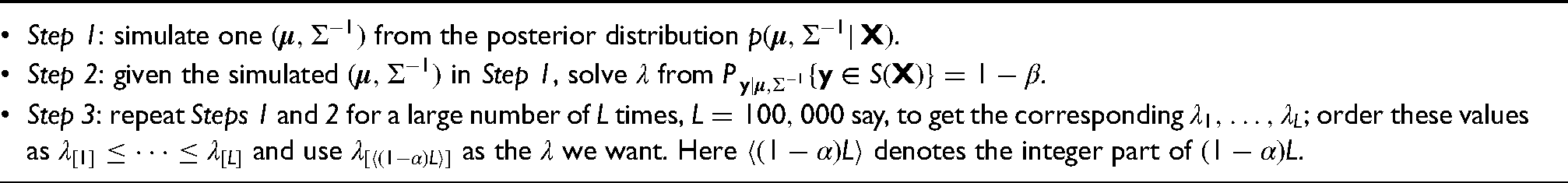
For computing $\lambda$ by simulation for given $\mathbf{X}$

Step 1: simulate one $(\mathit{\mu },{\mathrm{\Sigma }}^{-1})$ from the posterior distribution $p(\mathit{\mu },{\mathrm{\Sigma }}^{-1}|\mathbf{X})$ . Step 2: given the simulated $(\mathit{\mu },{\mathrm{\Sigma }}^{-1})$ in Step 1, solve $\lambda$ from $P_{\mathbf{y}|\mathit{\mu },{\mathrm{\Sigma }}^{-1}}\{\mathbf{y}\in S(\mathbf{X})\}=1-\beta$ . Step 3: repeat Steps 1 and 2 for a large number of $L$ times, $L=100,000$ say, to get the corresponding ${\lambda }_1,\dots ,{\lambda }_L$ ; order these values as ${\lambda }_{[1]}\le \cdots \le {\lambda }_{[L]}$ and use ${\lambda }_{[⟨(1-\alpha )L⟩]}$ as the $\lambda$ we want. Here $⟨(1-\alpha )L⟩$ denotes the integer part of $(1-\alpha )L$ .

We use a simulation method, given by Algorithm 3.2, to compute the $\lambda$ from (12). It is well known that the $(1-\alpha )$ sample quantile ${\lambda }_{[⟨(1-\alpha )L⟩]}$ in Algorithm 3.2 converges almost surely to the $(1-\alpha )$ population quantile $\lambda$ that solves (9) as $L\to \mathrm{\infty }$ . Hence ${\lambda }_{[⟨(1-\alpha )L⟩]}$ can be regarded as accurate so long as the number of simulations $L$ is large enough. The computation results given in (the penultimate paragraph of) Section 3.3 below show that $L=100,000$ is sufficiently large for the problem considered in this paper.

Now Step 1 can be implemented by using the distributional results in (2) and (3) in the following way. We first simulate one ${\mathrm{\Sigma }}^{-1}$ from $W_2([(n-1)V{]}^{-1},n-2)$ and then one $\mathit{\mu }$ from $N_2(\overline{\mathbf{x}},\mathrm{\Sigma }/n)$ to generate one $(\mathit{\mu },{\mathrm{\Sigma }}^{-1})$ . To simulate one ${\mathrm{\Sigma }}^{-1}$ from $W_2([(n-1)V{]}^{-1},n-2)$ , we use the Bartlett decomposition (see Smith and Hocking ³¹ and the references therein) in the following way. Step (a): generate independent random variables $u_{11}\sim {\chi }_{n-1}^2$ , $u_{22}\sim {\chi }_{n-2}^2$ and $u_{12}\sim N(0,1)$ to form matrix $U=\left(\begin{array}{c}\sqrt{u_{11}},u_{12}\\ 0,\sqrt{u_{22}}\end{array}\right)$ . Step (b): set ${\mathrm{\Sigma }}^{-1}=[(n-1)V{]}^{-1/2}{U}^{\prime }U[(n-1)V{]}^{-1/2},$ which has the required Wishart distribution. This simulation method for ${\mathrm{\Sigma }}^{-1}$ works for a general $k\ge 2$ . Alternatively one can directly use, for example, the R package rWishart.

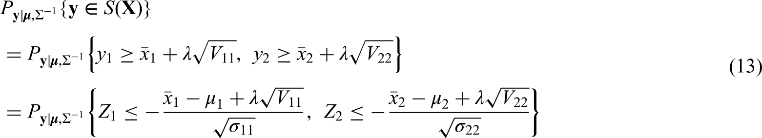
For Step 2, we have from (7) and (11) that

$$\begin{array}{rl}& P_{\mathbf{y}|\mathit{\mu },{\mathrm{\Sigma }}^{-1}}\{\mathbf{y}\in S(\mathbf{X})\}\\ & =P_{\mathbf{y}|\mathit{\mu },{\mathrm{\Sigma }}^{-1}}\{y_1\ge {\overline{x}}_1+\lambda \sqrt{V_{11}},y_2\ge {\overline{x}}_2+\lambda \sqrt{V_{22}}\}\\ & =P_{\mathbf{y}|\mathit{\mu },{\mathrm{\Sigma }}^{-1}}\{Z_1\le -\frac{{\overline{x}}_1-{\mu }_1+\lambda \sqrt{V_{11}}}{\sqrt{{\sigma }_{11}}},Z_2\le -\frac{{\overline{x}}_2-{\mu }_2+\lambda \sqrt{V_{22}}}{\sqrt{{\sigma }_{22}}}\}\end{array}$$

(13)where $Z_1=-(y_1-{\mu }_1)/\sqrt{{\sigma }_{11}}$ and $Z_2=-(y_2-{\mu }_2)/\sqrt{{\sigma }_{22}}$ have distribution $N_2(\mathbf{0},\left(\begin{array}{c}1,\rho \\ \rho ,1\end{array}\right))$ , with $\mathrm{\Sigma }=({\sigma }_{ij})$ and $\rho ={\sigma }_{12}/\sqrt{{\sigma }_{11}{\sigma }_{22}}$ . The probability in (13) can be computed directly by using the function pmvnorm of the R package mvtnorm; see Genz and Bretz ³² and Genz et al. ³³ for more details. Furthermore, note that this probability is monotone decreasing in $\lambda$ . Hence the unique solution $\lambda$ of $P_{\mathbf{y}|\mathit{\mu },{\mathrm{\Sigma }}^{-1}}\{\mathbf{y}\in S(\mathbf{X})\}=1-\beta$ can be easily computed by using a numerical searching algorithm, for example, the bisection method is used in our coding. From our experience, the computation of one $\lambda$ in Step 2 takes only a small fraction of a second on an ordinary personal computer (PC); see more details in the next subsection.

If one uses, in Step 2, an inner loop of simulation to compute an approximation to $\lambda$ , similar to an idea used in, for example, Krishnamoorthy and Mathew ²⁵ to construct the frequentist ellipsoidal tolerance region $R(\mathbf{X})$ , then the computation is much more time-consuming and the resultant $\lambda$ is much less accurate. Hence, this is not recommended for computing $\lambda$ .

3.3 Applications to the dataset on GH-2000 scores

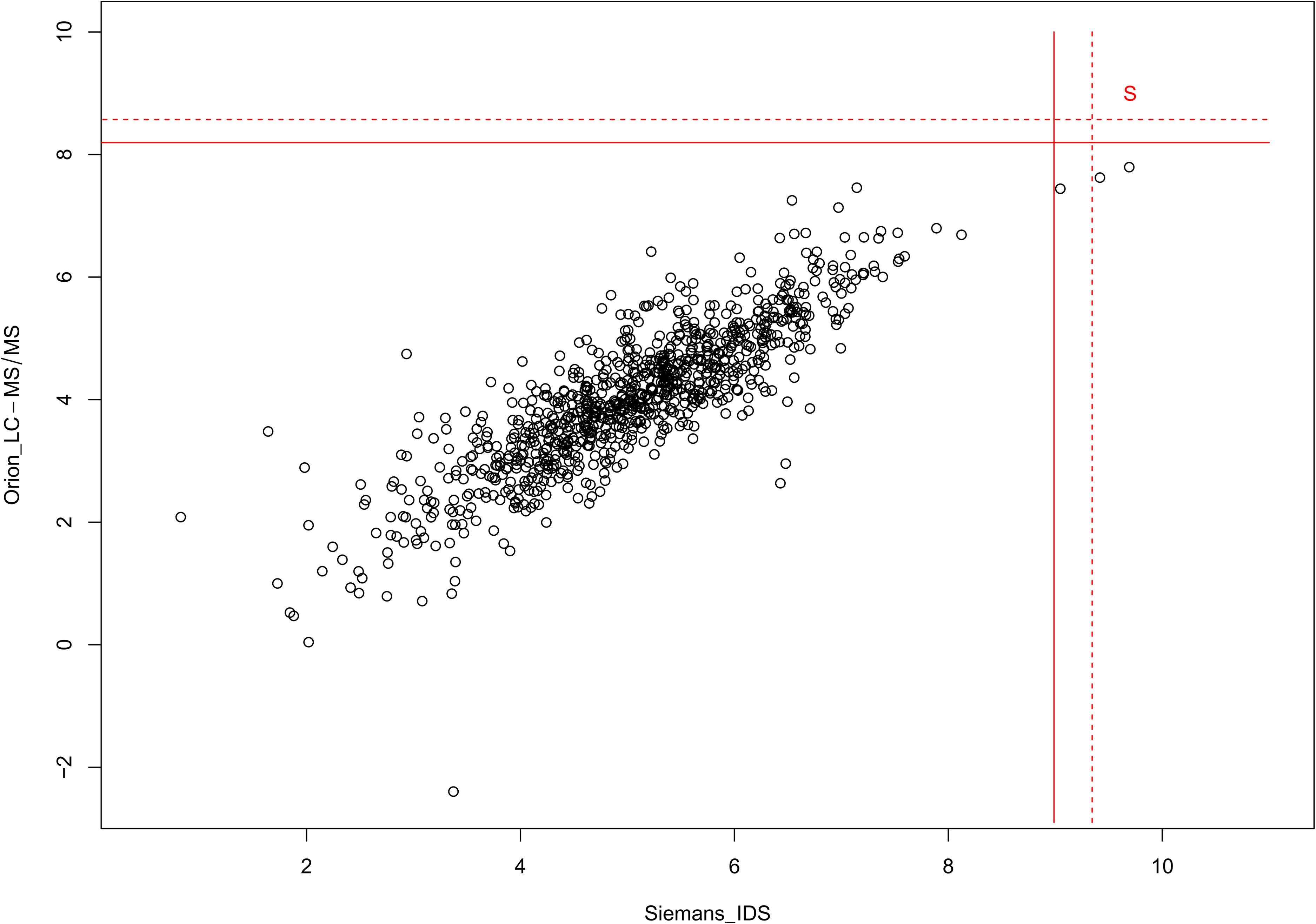
In this subsection, we compute the decision limits given in the last two subsections using the available sample observations on GH-2000 from Holt et al. ⁷ For the purpose of illustration, we focus on the following two GH-2000 scores: (1) Siemens IDS generated by using the P-III-NP assay Siemens ADVIA Centaur and IGF-I assay Immunodiagnostic Systems iSYS IGF-I and (2) Orion liquid chromatography-tandem mass spectrometry (LC-MS/MS) generated by P-III-NP assay UniQ ${}^{\text{TM}}$ P-III-NP RIA and IGF-I assay LC-MS/MS. These two GH-2000 scores are available for a sample of $n=917$ female athletes and plotted by the 917 dots in Figure 1. There were 932 female athletes in the sample originally. But some had Siemens IDS readings missing, and some had Orion LC-MS/MS readings missing. Hence, only the $n=917$ female athletes having both readings available are used in the analysis below.

Figure 1.

Plots of the single and combined decision limits based on the observed data. Single decision limits are given by the dotted lines. Combined decision limits are given by the upper-right quadrant $S$ bounded by two solid lines.

We set FPR $1-\beta =1/10,000$ and confidence level $1-\alpha =95\text{\%}$ , which are currently adopted by WADA. If one wants to use the GH-2000 score Siemens IDS ( $y_1$ ) only to decide whether a future female athlete with reading $\mathbf{y}=(y_1,y_2{)}^{\prime }$ is positive on GH misuse, then the single decision limit is computed from the formula in (6) and given by $a(\mathbf{X})=9.3445$ . It is depicted by the vertical dotted line in Figure 1. Hence, a future female athlete is judged to be positive if and only if $y_1>9.3445$ . If one wants to use the GH-2000 score Orion LC-MS/MS ( $y_2$ ) only to decide whether a future female athlete is positive, then the single decision limit is computed again from the formula in (6) and given by $a(\mathbf{X})=8.5703$ . It is depicted by the horizontal dotted line in Figure 1. Hence, a future female athlete is judged to be positive if and only if $y_2>8.5703$ .

On the other hand, if one wants to use both the GH-2000 scores Siemens IDS and Orion LC-MS/MS to decide whether a future female athlete with reading $\mathbf{y}=(y_1,y_2{)}^{\prime }$ is positive, then the combined decision limits in (11) are used and computed by using Algorithm 3.2. By using $L=100,000$ simulations, $\lambda$ is calculated to be 3.5578, which gives $a_1(\mathbf{X})=8.9881$ and $a_2(\mathbf{X})=8.1952$ . These two decision limits are depicted by the two solid lines, respectively, in Figure 1, and the set $S(\mathbf{X})$ is given by the upper-right quadrant formed by these two solid lines and indicated by the letter $S$ in the figure. Hence, a future female athlete is judged to be positive if and only if both $y_1>8.9881$ and $y_2>8.1952$ .

The decision limits constructed according to the property in (9) or (12) have the following interpretation. With $1-\alpha$ belief or confidence about the possible value of $(\mathit{\mu },\mathrm{\Sigma })$ that, the FPR is no more than 1 in 10,000 that a future athlete, whose GH-2000 reading $\mathbf{y}$ follows the distribution $N_2(\mathit{\mu },\mathrm{\Sigma })$ , is wrongly judged to be positive.

The computation of $\lambda$ based on $L=100,000$ simulations takes about 210 s on an ordinary Window’s PC (Intel(R) Core(TM) i5-6600 CPU 3.30GHz, RAM 8.0 GB). We have tried five different random seeds for the random number generator, which give the corresponding $\lambda$ -values: 3.5572, 3.5574, 3.5567, 3.5594, and 3.5579. This indicates that the $\lambda$ value computed using $L=100,000$ is likely to be accurate to the second decimal place at least. Indeed, one computation we have done using $L=1,000,000$ simulations produces $\lambda =3.5572$ and takes about 2210 s (37 min). Hence, the computation method proposed is fast and accurate enough for practical purposes with $L=100,000$ .

It is valuable to compare the proposed combined decision limits with the combined decision limits of Erotokritou-Mulligan et al. ¹¹ and Holt, ⁷ which is mentioned in Section 1. They are given by ${\tilde{a}}_1(\mathbf{X})={\overline{x}}_1+\tilde{\lambda }\sqrt{V_{11}}$ and ${\tilde{a}}_2(\mathbf{X})={\overline{x}}_2+\tilde{\lambda }\sqrt{V_{22}}$ , and so of similar form as the new combined decision limits given in (11). However, the critical constant is given by $\tilde{\lambda }=\tilde{k}+z_{1-\alpha }\sqrt{(1+{\tilde{k}}^2/2)/n}$ with $\tilde{k}$ being solved from $P\{W_1>\tilde{k},W_2>\tilde{k}\}=1-\beta$ , where $(W_1,W_2{)}^{\mathrm{\prime }}$ has distribution $N_2(\left(\begin{array}{c}0\\ 0\end{array}\right),\left(\begin{array}{c}1,\tilde{\rho }\\ \tilde{\rho },1\end{array}\right))$ with $\tilde{\rho }$ being the usual sample correlation coefficient between the two GH-2000 scores $x_1$ and $x_2$ based on the sample $\mathbf{X}$ . For the case considered in this subsection, it is computed that $\tilde{\rho }=V_{12}/\sqrt{V_{11}{V}_{22}}=0.852$ , $\tilde{k}=3.4049$ , $\tilde{\lambda }=3.5465$ , ${\tilde{a}}_1(\mathbf{X})=8.9755$ , and ${\tilde{a}}_2(\mathbf{X})=8.1820$ .

While ${\tilde{a}}_1(\mathbf{X})=8.9755$ and ${\tilde{a}}_2(\mathbf{X})=8.1820$ are quite close to $a_1(\mathbf{X})=8.9881$ and $a_2(\mathbf{X})=8.1952$ , respectively, for the specific sample observed, the construction of ${\tilde{a}}_1(\mathbf{X})$ and ${\tilde{a}}_2(\mathbf{X})$ does not guarantee that $\{\mathbf{y}:y_1\le {\tilde{a}}_1(\mathbf{X})\mathrm{or}{y}_2\le {\tilde{a}}_2(\mathbf{X})\}$ forms a $1-\alpha$ confidence and $\beta$ content tolerance region for the population $N_2(\mathit{\mu },\mathrm{\Sigma })$ . Indeed a simulation study in the next subsection shows that the true probability of $\{\mathbf{y}:y_1\le {\tilde{a}}_1(\mathbf{X})\mathrm{or}{y}_2\le {\tilde{a}}_2(\mathbf{X})\}$ covering $\beta$ content of the population $N_2(\mathit{\mu },\mathrm{\Sigma })$ could deviate from the nominal level $1-\alpha$ in both directions.

3.4 Simulation studies

In this subsection, a simulation study is carried out to assess whether the Bayesian $1-\alpha$ confidence and $\beta$ content tolerance region $\overline{S}(\mathbf{X})$ in Section 3.3 is also a frequentist $1-\alpha$ confidence and $\beta$ content tolerance region for $N_2(\mathit{\mu },\mathrm{\Sigma })$ . Specifically, we assess whether

$$P_{\overline{\mathbf{x}},V}\{P_{\mathbf{y}|\overline{\mathbf{x}},V}\{\mathbf{y}\in \overline{S}(\mathbf{X})\}\ge \beta \}\ge 1-\alpha$$

(14)holds for all possible values of $\mathit{\mu }$ and $\mathrm{\Sigma }$ ; here the probability $P_{\mathbf{y}|\overline{\mathbf{x}},V}\{\cdot \}$ is calculated with respect to $\mathbf{y}\sim N_2(\mathit{\mu },\mathrm{\Sigma })$ conditional on the sample mean and covariance matrix $(\overline{\mathbf{x}},V)$ , and $P_{\overline{\mathbf{x}},V}\{\cdot \}$ is calculated with respect to $(\overline{\mathbf{x}},V),$ which depends on the random sample $\mathbf{X}$ from $N_2(\mathit{\mu },\mathrm{\Sigma })$ .

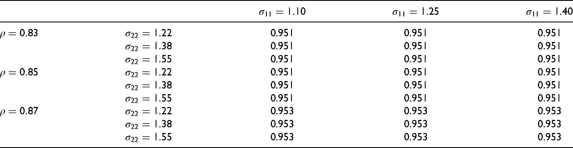
It can be shown that $P_{\overline{\mathbf{x}},V}\{P_{\mathbf{y}|\overline{\mathbf{x}},V}\{\mathbf{y}\in \overline{S}(\mathbf{X})\}\ge \beta \}$ does not depend on $\mathit{\mu }$ . Hence, it is only necessary to assess whether (14) holds for all possible values of $\mathrm{\Sigma }=(\begin{array}{c}{\sigma }_{11},\rho \sqrt{{\sigma }_{11}{\sigma }_{22}}\\ \rho \sqrt{{\sigma }_{11}{\sigma }_{22}},{\sigma }_{22}\end{array})$ with $\mathit{\mu }=0$ . From the observed sample on GH-2000 scores in Section 3.3, the 99% confidence intervals for $\rho$ , ${\sigma }_{11}$ and ${\sigma }_{22}$ are given, respectively, by $(0.827,0.874)$ , $(1.097,1.396)$ and $(1.215,1.546)$ . So the following three values $(0.83,0.85,0.87)$ are used for $\rho$ , $(1.10,1.25,1.40)$ for ${\sigma }_{11}$ , and $(1.22,1.38,1.55)$ for ${\sigma }_{22}$ in the simulation study, with a total of 27 combinations of $\mathrm{\Sigma }$ . The range of these 27 combinations cover the likely true value of $\mathrm{\Sigma }$ . Furthermore, FPR $1-\beta =1/10,000$ , confidence level $1-\alpha =95\text{\%}$ and sample size $n=917$ are used as in Section 3.3.

Algorithm 3.4.

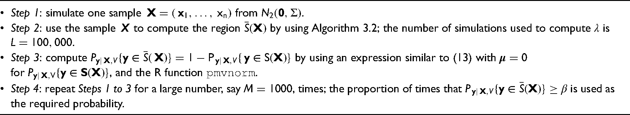
For computing the (outer) probability in (14) by simulation

Step 1: simulate one sample $\mathbf{X}=({\mathbf{x}}_1,\dots ,{\mathbf{x}}_n)$ from $N_2(\mathbf{0},\mathrm{\Sigma })$ . Step 2: use the sample $\mathit{X}$ to compute the region $\overline{S}(\mathbf{X})$ by using Algorithm 3.2; the number of simulations used to compute $\lambda$ is $L=100,000$ . Step 3: compute $P_{\mathbf{y}|\mathbf{X},\mathit{V}}\{\mathbf{y}\in \overline{S}(\mathbf{X})\}=1-P_{\mathbf{y}|\mathbf{X},\mathit{V}}\{\mathbf{y}\in S(\mathbf{X})\}$ by using an expression similar to (13) with $\mathit{\mu }=0$ for $P_{\mathbf{y}|\mathbf{X},\mathrm{V}}\{\mathbf{y}\in S(\mathbf{X})\}$ , and the R function pmvnorm. Step 4: repeat Steps 1 to 3 for a large number, say $M=1000$ , times; the proportion of times that $P_{\mathbf{y}|\mathbf{X},\mathit{V}}\{\mathbf{y}\in \overline{S}(\mathbf{X})\}\ge \beta$ is used as the required probability.

The (outer) probability $P_{\overline{\mathbf{x}},V}\{\cdot \}$ in (14) is approximated by a proportion using Algorithm 3.4. It takes about 60 h to compute each probability in Table 1 on the same computer as mentioned in Section 3.3, with most computation time spent on computing the $\lambda$ -values in the $M=1000$ repetitions.

Table 1.

The probability in (14) for given $\mathrm{\Sigma }$ .

		${\sigma }_{11}=1.10$	${\sigma }_{11}=1.25$	${\sigma }_{11}=1.40$
$\rho =0.83$	${\sigma }_{22}=1.22$	0.951	0.951	0.951
	${\sigma }_{22}=1.38$	0.951	0.951	0.951
	${\sigma }_{22}=1.55$	0.951	0.951	0.951
$\rho =0.85$	${\sigma }_{22}=1.22$	0.951	0.951	0.951
	${\sigma }_{22}=1.38$	0.951	0.951	0.951
	${\sigma }_{22}=1.55$	0.951	0.951	0.951
$\rho =0.87$	${\sigma }_{22}=1.22$	0.953	0.953	0.953
	${\sigma }_{22}=1.38$	0.953	0.953	0.953
	${\sigma }_{22}=1.55$	0.953	0.953	0.953

Table 1 presents the simulation results on the probability in (14). It is clear from Table 1 that the probabilities are very close to $1-\alpha =0.95$ for all the 27 configurations of $\rho ,{\sigma }_{11}$ and ${\sigma }_{22}$ . Since the range of these 27 configurations most likely covers the true value of $\mathrm{\Sigma }$ , it follows therefore that it is most likely the inequality in (14) holds for the unknown true value of $\mathrm{\Sigma }$ . Hence the Bayesian combined decision limits can also be interpreted as the frequentist combined decision limits of approximate $1-\alpha$ confidence.

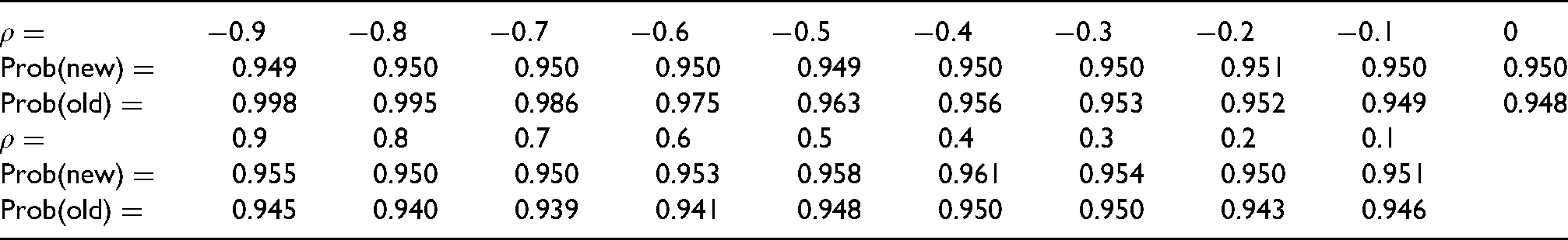
The results in Table 1 seem to indicate that the probability in (14) depends on $\mathrm{\Sigma }$ , that is, ${\sigma }_{11},{\sigma }_{22}$ and $\rho$ , only through $\rho$ . But this is difficult to prove analytically since the critical constant $\lambda$ of $S(\mathbf{X})$ depends on $\mathrm{\Sigma }$ in a complicated manner in Step 1 of Algorithm 3.2. We have done further simulation study on the probability in (14) with ${\sigma }_{11}={\sigma }_{22}=1$ and various values of $\rho$ in the wider range $[-0.9,0.9]$ . The results are given by Prob (new) in Table 2.

Table 2.

The probability in (14) for given $\mathrm{\Sigma }$ with ${\sigma }_{11}={\sigma }_{22}=1$ .

$\rho =$	$-0.9$	$-0.8$	$-0.7$	$-0.6$	$-0.5$	$-0.4$	$-0.3$	$-0.2$	$-0.1$	0
$\mathrm{Prob}(\mathrm{new})=$	0.949	0.950	0.950	0.950	0.949	0.950	0.950	0.951	0.950	0.950
$\mathrm{Prob}(\mathrm{old})=$	0.998	0.995	0.986	0.975	0.963	0.956	0.953	0.952	0.949	0.948
$\rho =$	0.9	0.8	0.7	0.6	0.5	0.4	0.3	0.2	0.1
$\mathrm{Prob}(\mathrm{new})=$	0.955	0.950	0.950	0.953	0.958	0.961	0.954	0.950	0.951
$\mathrm{Prob}(\mathrm{old})=$	0.945	0.940	0.939	0.941	0.948	0.950	0.950	0.943	0.946

The results on Prob (new) in Table 2 indicate that, if the probability in (14) does depend on $\mathrm{\Sigma }$ only through $\rho$ , then this probability seems to be quite close to $1-\alpha =0.95$ across the wide range $[-0.9,0.9]$ of $\rho$ -values.

Finally, we have carried out a simulation study to assess the probability corresponding to the probability in (14) but for the combined decision limits ${\tilde{a}}_1(\mathbf{X})$ and ${\tilde{a}}_2(\mathbf{X})$ of Erotokritou-Mulligan et al. ¹¹ and Holt. ⁷ It is clear that this probability depends on $\mathrm{\Sigma }$ only through $\rho$ , and the simulation results on this probability are given by Prob (old) in Table 2. As pointed out in the last subsection, its construction does not guarantee that $\{\mathbf{y}:y_1\le {\tilde{a}}_1(\mathbf{X})\mathrm{or}{y}_2\le {\tilde{a}}_2(\mathbf{X})\}$ is a $1-\alpha$ confidence and $\beta$ content tolerance region for the population $N_2(\mathit{\mu },\mathrm{\Sigma })$ . From the results in Table 2, it can be seen that the probability of $\{\mathbf{y}:y_1\le {\tilde{a}}_1(\mathbf{X})\mathrm{or}{y}_2\le {\tilde{a}}_2(\mathbf{X})\}$ covering $\beta =0.9999$ content of the population $N_2(\mathit{\mu },\mathrm{\Sigma })$ tends to be a bit smaller than the nominal level $1-\alpha =0.95$ when the true value of $\rho$ is around 0.7. Strong deviations from the nominal level occur for $\rho$ smaller than $-0.5$ . In practice, negative correlations between two GH-2000 scores are unlikely to occur. But in other applications where the two scores have a large negative correlation, the method of Erotokritou-Mulligan et al. ¹¹ and Holt ⁷ will produce ${\tilde{a}}_1(\mathbf{X})$ and ${\tilde{a}}_2(\mathbf{X})$ that are larger than necessary. In contrast, with the new combined decision limits, the probabilities Prob(new) are consistently close to the nominal level across the range of $\rho$ values.

4 Discussion

Decision limits based on the GH-2000 scores produced by the various pairs of analytical assays employed have been published. These scores are used individually but scores for two pairs of assays must be exceeded before an athlete has to answer a case for the misuse of GH. In other words, WADA mandated the measurement of each analyte by two methods which meant that each sample had two GH-2000 scores. Hence, it is natural to use the correlation structure involved in the two scores to develop naturally decreased decision limits which would increase the sensitivity of the biomarker method. The biomarker test then would be more sensitive the lower the correlation between the two GH-2000 scores under consideration would be.

While combined decision limits have their benefits there are some drawbacks. First, depending on which of the other pair of assays was used, the decision limit for one assay pair could change and that could lead to confusion. Ideally, for a given GH-2000 score one would like to have a unique decision limit and not one that depends on which other GH-2000 score is used in the pair. Secondly, it became possible to measure IGF-I by mass spectrometry as the preferred choice to measure IGF-I. WADA does not mandate measurement by a second assay when an analyte is measured by mass spectrometry because of the greater reliability and traceability of the method compared with immunoassays. Hence, using the same assay for IGF-I in two GH-2000 scores leads to an increase in the correlation and the potential for an increased sensitivity of the biomarker test diminishes. On the other hand, it might be that in the near future two mass spectrometric methods for IGF-I (intact and digest) will be available with a potential of a decrease in the correlation of two GH-2000 scores involved in the pair.

Having said that, it is valuable nevertheless to have a statistical theory for constructing combined decision limits. These combined decision limits should have the same pre-specified $1-\alpha$ confidence and $1-\beta$ FPR as the single decision limit. A Bayesian approach is used in this paper to construct the combined decision limits. Our simulation study in Section 3.4 shows that the Bayesian combined decision limits also have satisfactory frequentist properties and so can be regarded as frequentist combined decision limits too. The R code available from the authors allows the method ready to be used.

Combined decision limits of other forms are worth investigating too in future. For example, it seems also sensible to use combined decision limits of the form $T(\mathbf{X})=\{\mathbf{y}:y_1>a_1(\mathbf{X})\mathrm{or}{y}_2>a_2(\mathbf{X})\}$ with $a_1(\mathbf{X})$ and $a_2(\mathbf{X})$ of the forms in (11). That is, a future athlete is judged to be positive if either of the two readings is too high. The corresponding $\overline{T}(\mathbf{X})$ becomes a one-sided rectangular tolerance region for a bivariate normal distribution considered recently in Lucagbo ²⁸ (Section 4.7). It would be interesting to compare the tolerance region $\overline{T}(\mathbf{X})$ constructed using the Bayesian method as in this paper with the tolerance region $\overline{T}(\mathbf{X})$ constructed using parametric bootstrap of Lucagbo. ²⁸

The computation method of Section 3.2 can potentially be explored in the construction of a frequentist tolerance region of the ellipsoidal form $R(\mathbf{X})$ in (10) for $k=2$ at least, which is probably the most useful case in applications of tolerance regions. Furthermore, the construction of the Bayesian tolerance region of the ellipsoidal form $R(\mathbf{X})$ can also be investigated, even though it is not of direct interest to GH misuse detection.

While the GH misuse detection motivates this work, one can envisage other potential applications of the methodology developed in this paper. For example, suitable decision limits can be constructed to trigger an alert on whether a child of a given age is over/underweight or over/underheight.

For nonparametric tolerance regions, the reader is referred to Young and Mathew, ²⁹ Lucagbo ²⁸ (Chapter 5) and Chen ³⁰ (Chapter 3) for the latest development.