
Abstract
Meta-analysis of randomized controlled trials is generally considered the most reliable source of estimates of relative treatment effects. However, in the last few years, there has been interest in using non-randomized studies to complement evidence from randomized controlled trials. Several meta-analytical models have been proposed to this end. Such models mainly focussed on estimating the average relative effects of interventions. In real-life clinical practice, when deciding on how to treat a patient, it might be of great interest to have personalized predictions of absolute outcomes under several available treatment options. This paper describes a general framework for developing models that combine individual patient data from randomized controlled trials and non-randomized study when aiming to predict outcomes for a set of competing medical interventions applied in real-world clinical settings. We also discuss methods for measuring the models’ performance to identify the optimal model to use in each setting. We focus on the case of continuous outcomes and illustrate our methods using a data set from rheumatoid arthritis, comprising patient-level data from three randomized controlled trials and two registries from Switzerland and Britain.
Keywords
Introduction
Randomized clinical trials (RCTs) and meta-analyses (MAs) of clinical trials are usually thought to be the most reliable source of evidence to evaluate the effects of medical interventions. 1 However, RCTs are often carried out in specific settings and apply strict inclusion and exclusion criteria, which leads to results that may not be generalizable to routine practice. 2 This situation leads to the so-called efficacy-effectiveness gap,3,4 where ‘efficacy’ refers to the performance of a medical intervention under experimental conditions, while ‘effectiveness’ relates to what is achieved in everyday clinical practice.
In the last few years, there has been growing interest in utilizing ‘real-world’ data from non-randomized studies (NRSs), to complement evidence from RCTs in medical decision-making, aiming to bridge the efficacy-effectiveness gap.5–8 The increased interest in NRSs was accompanied by the development of various meta-analytical modelling approaches,9–12 and by extending methods to network meta-analysis (NMA) and individual patient data (IPD) MA.13–15 So far, methods have primarily focussed on estimating relative treatment effects. When making (shared) decisions 16 on how to treat patients in real-world settings, the prediction of (possibly several) outcomes under all competing treatments for individual patients or specific groups of patients is of great interest. In this context, jointly synthesizing IPD from RCTs and non-randomized, real-world studies in a prediction framework is promising. This idea was previously explored by Didden et al., 17 who aimed to predict the average, population-level, real-world effectiveness of a treatment pre-launch (i.e. before a treatment becomes available for clinical practice). However, to the best of our knowledge, there are no methods that combine patient-level data from multiple studies, randomized and observational, to provide personalized predictions for various treatments for patients treated in real-world settings.
We set out to fill this gap and propose a general prediction framework. We extend prediction modelling methods to an NMA setting 18 to synthesize evidence on multiple interventions, utilizing IPD from randomized and NRSs. We propose a range of modelling approaches for predicting real-world outcomes and describe methods for selecting the optimal model to use. We focus on two-stage models, where at the first stage each study is analysed separately, and at the second stage the study-specific results are meta-analysed. Although one-stage approaches to IPD-MA and IPD-NMA are generally considered more flexible, 19 a two-stage approach is often necessary for practice, due to data restrictions, e.g. when data reside on different servers. We illustrate how to implement our framework, using a real example in rheumatoid arthritis (RA), combining data from multiple trials and registries.
A clinical example in RA
We used IPD from three RCTs and two NRS (based on disease registries) on patients diagnosed with RA, a chronic inflammatory disease characterized by progressive damage of joints. 20 Several drugs can be prescribed for the treatment of RA. In this example, we focus on three: conventional synthetic disease-modifying anti-rheumatic drugs (DMARDs), combination therapy with rituximab (RTX) + DMARDs, and a combination of tocilizumab (TCZ) + DMARDs. Note that RTX and TCZ are also DMARDs, but they are biologic in contrast to conventional DMARDs such as methotrexate, which we refer to as DMARDs. The outcome of interest was the Disease Activity Score 28 (DAS28), 21 which is continuous and ranges from 0 to 10. A lower score indicates lower disease activity.
One RCT (REFLEX) compared RTX + DMARDs versus DMARDs and included 517 patients. The other two RCTs (TOWARD and TOWARD2) compared TCZ + DMARDs versus DMARDs, and included 1216 and 791 patients, respectively. In all three RCTs, DAS28 was at baseline and after 6 months. For the two NRS, we used the measurement of DAS28 at 6 month (or the closest available measurement, within 3 months) after the start of the new drug. The British Society for Rheumatology Biologics Register in Rheumatoid Arthritis (BSRBR-RA) and the Swiss Clinical Quality Management in Rheumatoid Arthritis (SCQM) registries provided observational data.22,23 These included 2057 and 1069 patients, respectively. Established in 2001, BSRBR-RA is one of the largest studies looking at the long-term safety of new drugs prescribed for RA. It was launched when anti-tumor necrosis factor (TNF) therapies became available. 21 Similarly, SCQM is a Swiss registry established in 1997 and allowed rheumatologists to follow their RA patients to improve outcomes. 22 In addition to baseline DAS28, nine patient-level covariates were available from both RCTs and NRS at baseline: gender, age, disease duration, body mass index, baseline rheumatoid factor, number of previous DMARDs and anti-TNF agents, baseline health assessment questionnaire disability index, and baseline erythrocyte sedimentation rate (ESR). We provide additional details on the studies in Tables 1–3 of the Appendix. Figure 1 shows the network graph and overview of data sets.
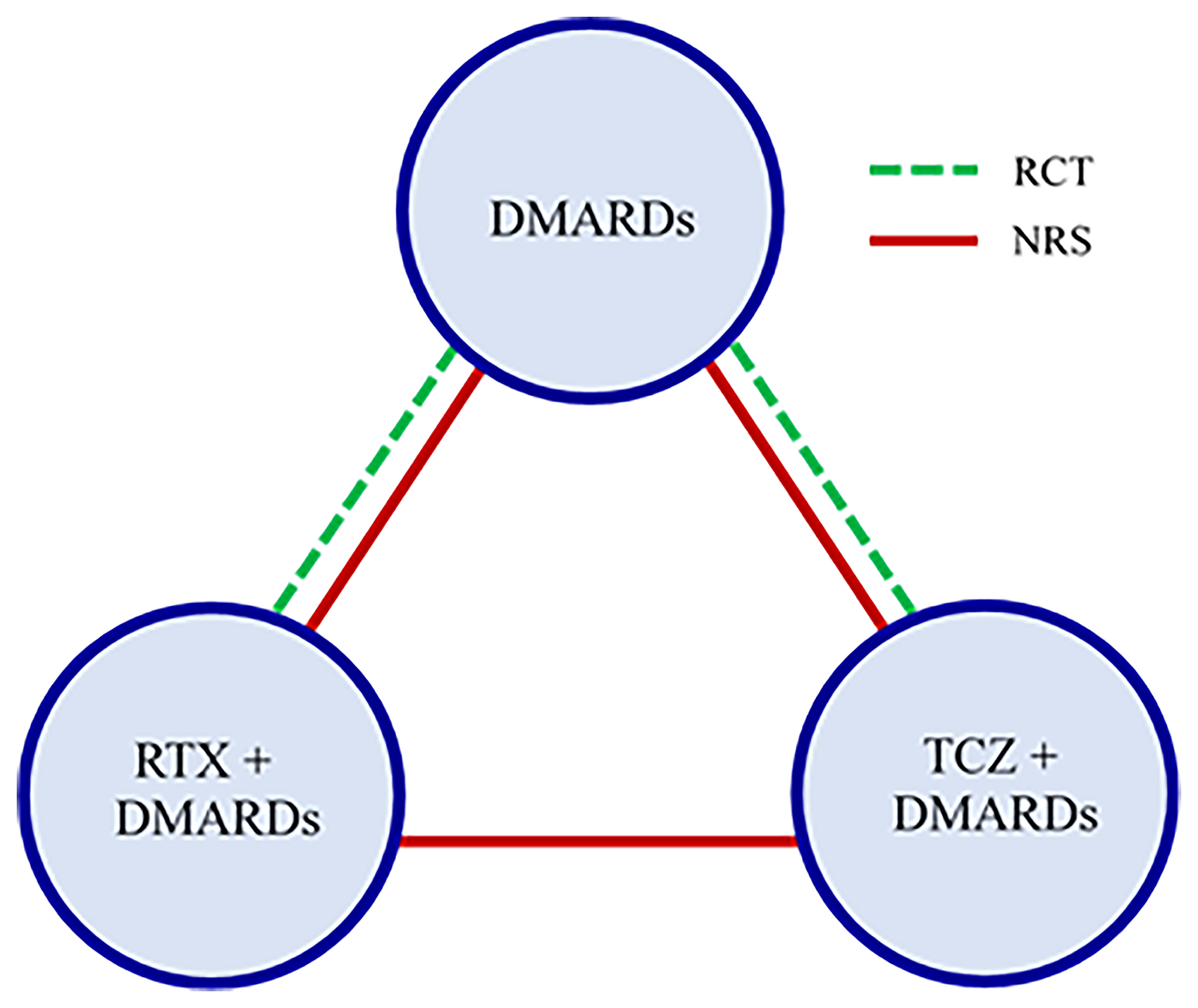
Network graph for the rheumatoid arthritis example. Green lines show RCTs and red lines show NRS. There were three two-armed RCTs; two of them compared TCZ + DMARDs vs DMARDs and one compared RTX + DMARDs vs DMARDs. There were two NRS, which included all three drugs. Abbreviations: DMARDs: Conventional disease-modifying anti-rheumatic drugs; RTX: rituximab; TCZ: tocilizumab; RCT: randomized controlled trial; NRS: non-randomized study.
Methods
Overview
Below, we propose a statistical framework to facilitate personalized medicine when IPD from NRS and RCTs are available. This framework can be used to build a multivariable model that predicts (absolute) patient-level, real-world outcomes for a range of different treatments for a given disease. We assume that the available data are IPD from a set of RCTs and NRS that compare two or more treatments for the same disease. The final product of our analyses will be a model where the input is a vector of patient-level covariates , and the output is the predicted outcome under each treatment . In what follows, we focus on the case of a continuous outcome and we limit our investigation to models with linear functions of the covariates. The model is as follows:

We describe a range of meta-analytical two-stage approaches that can be used to estimate the parameters in the prediction model of Equation (1). First, we analyse each study separately. Second, we meta-analyse the study-specific estimates, to estimate all parameters needed for Equation (1).
We focus on Bayesian approaches because of their flexibility and ease of propagating uncertainty. We describe three generic approaches for building prediction models that combine IPD from studies of variable design.
Approach I: We only use the IPD from a single NRS, i.e. without using MA. Approach II: We combine the IPD from all studies (NRS and RCTs) using a two-stage NMA, considering three different implementations. In approach IIa, we do not account for differences in study design. In approach IIb we employ shrinkage methods. In approach IIc, we further calibrate
24
the intercept and main effects of covariates to target a specific patient group, using data from a single NRS that reflects this population. Approach III: We combine the IPD from NRS and RCTs using a two-stage NMA and adopt a weighting scheme to account for different study designs (IIIa). Again, we allow for re-calibrating the intercept term and main effects of covariates to target a specific patient group (IIIb).
As an additional, simplified method, we combine all studies as in IIa but we do not include any treatment-covariate interactions, i.e. we set . We call this Approach IV. After describing the various approaches in detail, we discuss ways of assessing their performance. Table 1 summarizes each approach, briefly describing the model and citing equations used.
Overview of the different modelling approaches presented in this paper.
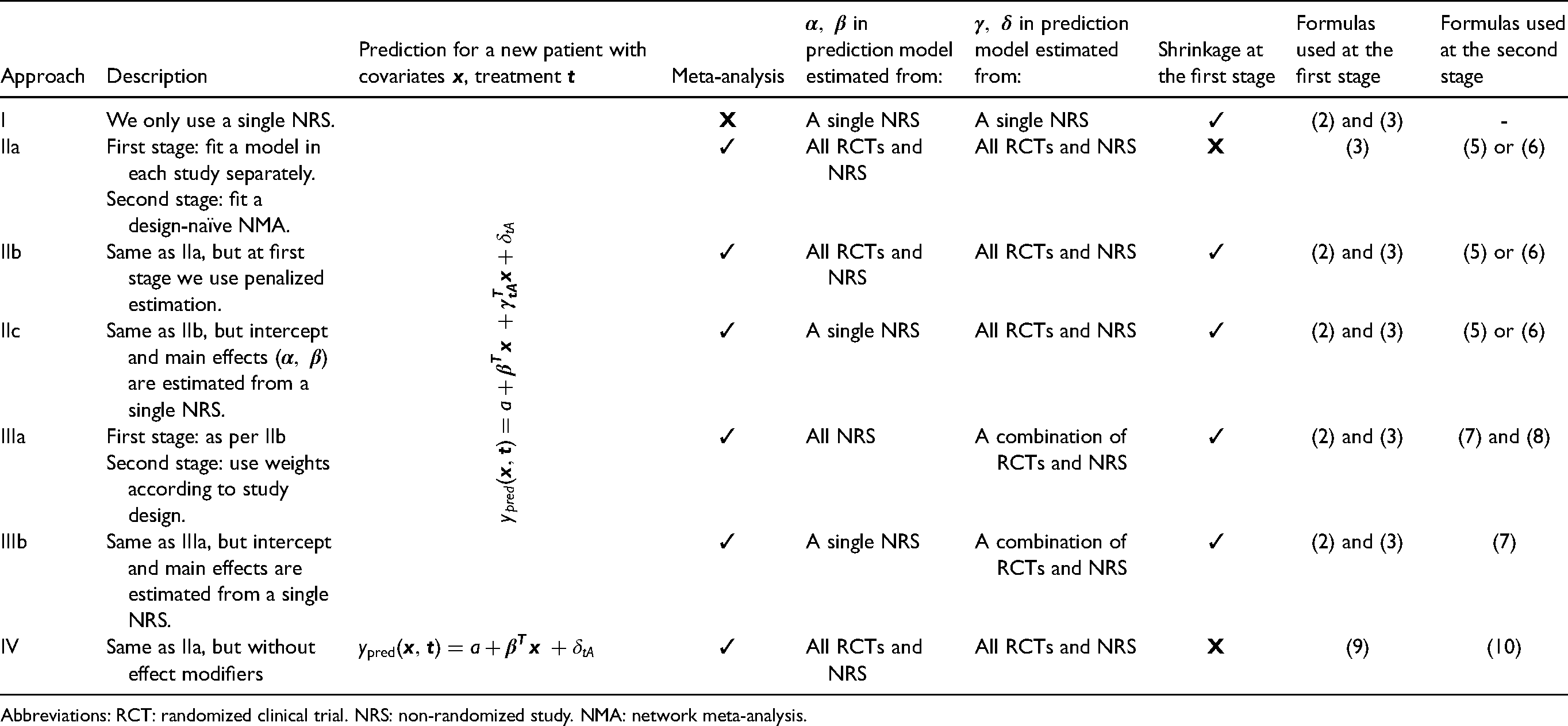
Abbreviations: RCT: randomized clinical trial. NRS: non-randomized study. NMA: network meta-analysis.
Approach I: Analysis of a single study, reflecting the target population
Let us assume that our aim is to predict outcomes for a real-world population from which we have a representative sample, including patient-level data (e.g. from a specific registry). We can build a prediction model using these data alone (e.g. the model of Equation (1)) and disregard all other sources of information. This approach is relatively common in the literature, although (a) usual applications do not account for multiple interventions, and (b) these models are often based on IPD from a single RCT.
To enhance the predictive performance of the model, we can incorporate shrinkage in the model estimation. Shrinkage methods are known to improve prediction accuracy,24,25 while it has been recently shown that they can be useful in a MA setting, when aiming to estimate patient-level treatment effects. 26 We are particularly interested in shrinking treatment-covariate interactions because information on effect modification is important, as it may substantially affect decision making.
There are many different frequentist as well as Bayesian shrinkage methods we could use. For example, for Bayesian shrinkage, we can penalize the coefficients of the effect modification (treatment-covariate interactions, i.e. parameters in Equation (1)) using a Laplace prior distribution. When the scale parameter of the Laplace prior distribution is assigned its own prior distribution, the model is often referred to as a Bayesian LASSO.27,28 The prior for effect modifiers of treatment W versus the reference A is given by:
Approach II: Design-naïve NMA
In this approach, we use all studies to fit a two-stage IPD NMA model. 30 We disregard the information on study design, i.e. we treat RCTs and NRS the same. Thus, we use all studies to inform parameters , , in Equation (1). The parameter of this model, which denotes the predicted outcome for zero value of the covariates under the reference treatment A, will only be informed by studies that included this treatment. This means that the choice of reference treatment is potentially important (while the choice of reference is arbitrary in the standard NMA model. 18 ) An obvious choice A is the treatment that is given to most patients across the available data sets.
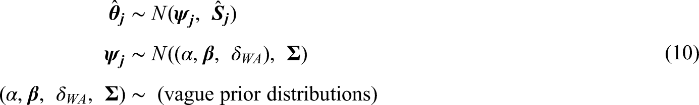
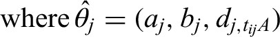
Let us assume that patient i was included in the study j, received treatment , and that for this patient the observed outcome of interest was , measured on a continuous scale. Also, we assume that for this patient we have covariates. Let us also assume that the study had only two treatment arms, W and A (the reference). Under these definitions, the first stage model is as follows: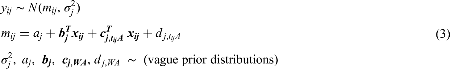
These estimates contribute to the likelihood of the second stage of the MA, via a multivariate random-effects model: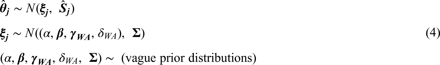
Furthermore, a typical assumption in NMA is that the between-study variance of the random effects is the same across treatment contrasts.
18
Then, the second stage model can be written as follows:
Again, it may be difficult to estimate heterogeneity of the treatment effect when only a few studies are available. This is the case for the RA example described in the ‘A clinical example in RA’ section. One solution would be to use external information to create an informative prior distribution for . For example, for the case of binary outcomes, Turner et al.
31
proposed empirical distributions that can be used in Bayesian MAs. A further simplification would be to assume common :
Lastly, we can further extend Approach IIb by calibrating the intercept and main effects of covariates to target a specific real-world population. A motivation for this is that data sampled from the patient population of interest might be the best source of evidence for predicting the reference treatment outcome. Conversely, estimates of the intercept term obtained from RCTs might be less representative for the target population because RCT patients are selected and because RCTs are performed in highly controlled settings.
In detail, we use Approach I to estimate , using only data obtained from a study that reflects the target population, and Approach IIb, using all data to estimate , . We then use Equation (1) to make predictions for individual patients. We call this Approach IIc. To summarize, in Approach IIc we use study-specific estimates of , and pooled relative effects, i.e. , . Note that we fit the full model within each study separately, and then pool all parameters (including all main effects and interactions) in the second stage of the model across studies. Table 1 summarizes all the different flavours of Approach II.
Approach III: Design-adjusted analysis
For Approach III, when aggregating parameters at the second stage, we use a weighting scheme for studies of a different design. 15 Specifically, we weight the first-stage estimates of relative treatment effects from Approach IIb according to the corresponding study's design.
In this approach, the variance of the estimates of treatment effects and effect modification obtained from NRS j (i.e. the variance of , ) is inflated after dividing by a factor , with . By doing so, we effectively decrease the impact of NRS in the estimation of all relative treatment effects. Setting corresponds to completely disregarding estimates of relative treatment effects obtained from NRS.
This approach's motivation is that RCTs are usually thought to be the most reliable sources of information for relative treatment effects because randomization helps us avoid issues related to confounding. Moreover, since we aim to predict outcomes for real-world populations, estimates for the model's intercept and the main effects of the covariates are aggregated only using NRS. The second stage model is as follows: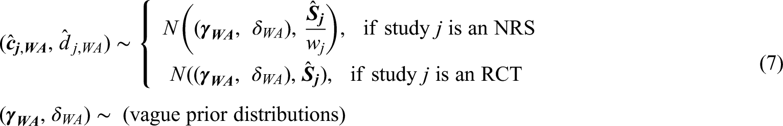

Approach IV: Design-naïve NMA without effect modifiers
For Approach IV, we fit the similar design-naïve NMA, but without including effect modifiers (i.e. setting ). This may serve as a sensitivity analysis, and by comparing its results with the previous methods we might obtain insights on the extent of heterogeneity of treatment effects. The linear predictor is now
Assessing the performance of the prediction models
A common practice to measure a prediction model's performance for a continuous outcome is through mean squared error (MSE) and bias:
We can also calculate the coefficient of determination (R-squared) to evaluate a model's performance for a given study of interest. We do that by using only and from each model:

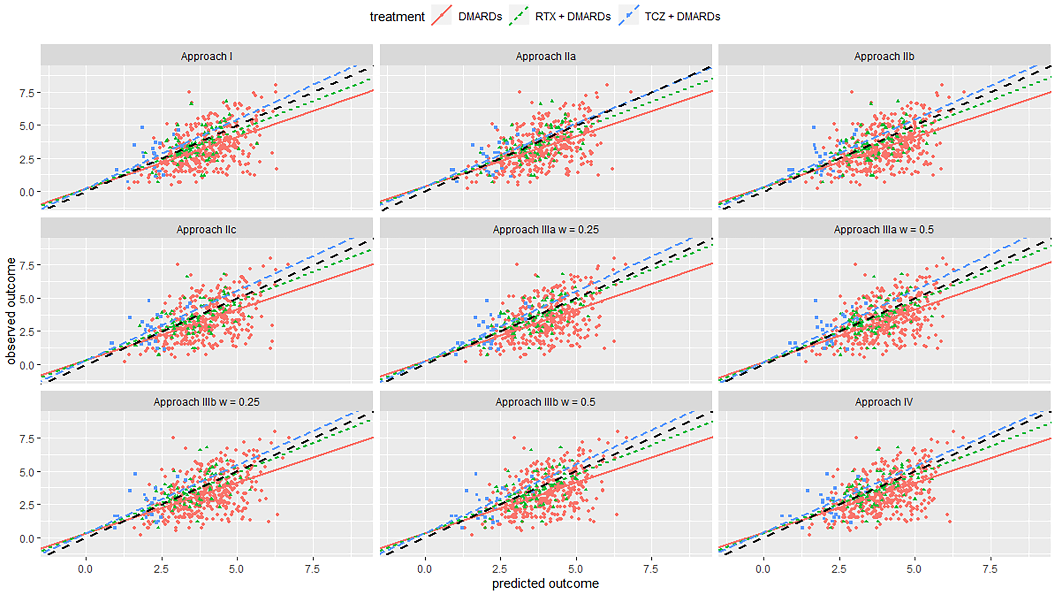
The performance measures in equations (11), (12), and (13) inform us of our models’ overall predictive ability. However, when deciding on how to treat, we are mainly interested in selecting the best treatment for each patient. Thus, a prediction model that would be useful for deciding between competing treatments should also be well calibrated in terms of estimated treatment benefit. To achieve this, we reshape the calibration line using the predicted benefit (i.e. the difference between predicted outcomes under different treatments). For networks with treatments , , , … for each of the competing models we fit the line
Cross validation
For each competing model, we can calculate the performance metrics discussed above using internal as well as an internal–external cross validation.32,33
For internal validation, we use all available data to develop the models. Then, given that we aim to predict real-world outcomes, we use the NRS to test all models, i.e. to compare predictions with observations using the measures described in the previous section. To correct for optimism, 24 we can calculate optimism-corrected performance using bootstrapping as discussed by Steyerberg. 24 More details on this procedure are given in Section 2.2 of the Appendix. An internal validation procedure will inform us on which model performs best for each specific setting, provided we stratify the procedure by study.
For internal-external cross-validation, we exclude one NRS from the analysis and use the rest of the data to train the models. We then use the left-out NRS to make predictions and compare them with observations. Finally, we cycle through all available NRS. To follow this approach, we need data from multiple NRS to be available. If this is not the case, we may split the single NRS data in a meaningful non-random way, e.g. by clinic, region, or any other clustering variable in our data set. This internal-external validation procedure can potentially provide insights on which model might perform better in new settings.
The internal–external cross-validation via leave-one-study-out cannot be combined with Approach I, as this analysis only uses a single study to train the model. In this case, we can instead use all NRS except the left-out one to develop the model. For instance, for the RA case study, we only used the British registry to train the model and the Swiss registry to make predictions, and vice versa. Moreover, for Approach IIc and IIIb, when using internal-external cross-validation, we use all NRS except the left-out to estimate intercept and main effects of covariates, i.e. we do not use RCTs.
Implementation details
Below we provide some details on implementing the described models in the RA example.
Standardization of covariates
To use penalized estimation in the analysis of study j we need to standardize variables. This is necessary to ensure that penalization is equally applied to all regressors. 25 Standardizing means transforming each covariate in each study by subtracting the study-specific mean from the covariate and dividing the result with the covariate's study-specific standard deviation. However, standardizing makes it difficult to MA results from multiple studies coherently, given that in each study the covariates are transformed differently. Thus, before aggregating the first stage results at the second stage, we need to revert coefficients to their natural scale. The mathematical details of how to do this are provided in Section 2.3 of the Appendix.
Imputation of missing data
Gelman et al. 34 recommended the following approach to handle missing data in Bayesian analyses via Markov Chain Monte Carlo (MCMC): (a) create m multiply imputed data sets; (b) analyse each imputed data set separately; (c) combine the m posterior draws, i.e. by mixing the corresponding draws.
We use R package mice 35 to impute the missing covariates to create multiply imputed data sets. 36 When imputing we used information from covariates, treatment, covariate-treatment interactions, and outcomes, but we did not impute the missing outcomes for model development. Imputation was done in each study separately using the method of predictive mean matching.
Fitting the models
All analyses were carried out in R
37
using
For all models, we used a vague prior distribution for the standard deviation of continuous outcomes (). For regression parameters of stage one (i.e. , , , and ), we used a distribution. When applying Bayesian LASSO in stage one, a vague prior distribution was placed on the scale parameter for Laplace prior (). We tested the sensitivity of results to the selection of prior distribution on . For Approach III, we used weights 0.25 and 0.5.
For calculating optimism-corrected performance, 200 bootstrap samples were drawn. The R codes used for fitting all models are available at https://github.com/MikeJSeo/phd/tree/master/ra.
Results
The parameter estimates from the first-stage analysis for each study are shown in Tables 4, 5, 6, and 7 in the Appendix. There were some important differences between RCTs and NRS, especially in the case of the Swiss registry. Τhe estimated intercept term for this study was much smaller than for the RCTs, probably owing to the fact that the Swiss registry had the lowest average DAS28 score; see Table 3 in the Appendix. Moreover, the average relative treatment effects of the biologic treatments versus DMARDs estimated in the registries were smaller than in the RCTs. These differences might raise concerns about the direct applicability of the RCT findings in patients found in real-world settings. We might hypothesize that these differences were due to residual confounding, model misspecification (e.g. omission of non-linear or interaction terms), or due to the more general ‘efficacy-effectiveness gap’ described in the Introduction.
Furthermore, there was only very weak evidence of heterogeneous treatment effects (i.e. effect modification) across all studies. Results from the second-stage analysis are shown in Table 8 of the Appendix. As expected, given the first stage results, methods that gave more weight to the RCTs in the estimation of relative effects provided larger effects. Next, we assessed all models’ performance using the measures described in the ‘Assessing the performance of the prediction models’ section and following the two cross-validation approaches described in the ‘Cross validation’ section.
We first discuss the results from the internal validation. In Table 2, we give results in terms of MSE and Bias, and in Table 3 results for the calibration lines and R-squared value. Figures 1 and 2 in the Appendix show the calibration plots. Overall, we saw that for most approaches the bias was rather small in clinical terms. MSE was around 1.5 for all models; to bring it to the same scale as the outcome we can calculate the root of MSE, i.e. 1.22, deemed to be small-to-moderate in clinical terms. R-squared was moderate (around 0.30 for all approaches). Moreover, we see that most models had similar performance. For the Swiss registry, Approach I performed slightly better for most measures of performance. For the British registry, approach IIIa was overall the best, especially in measures of calibration. However, differences with other methods, including Approach I, were not very pronounced. This showed that, when predicting real-world outcomes, utilizing data from multiple studies and using advanced analysis methods brought no benefit to the Swiss and small benefits to the British registry.
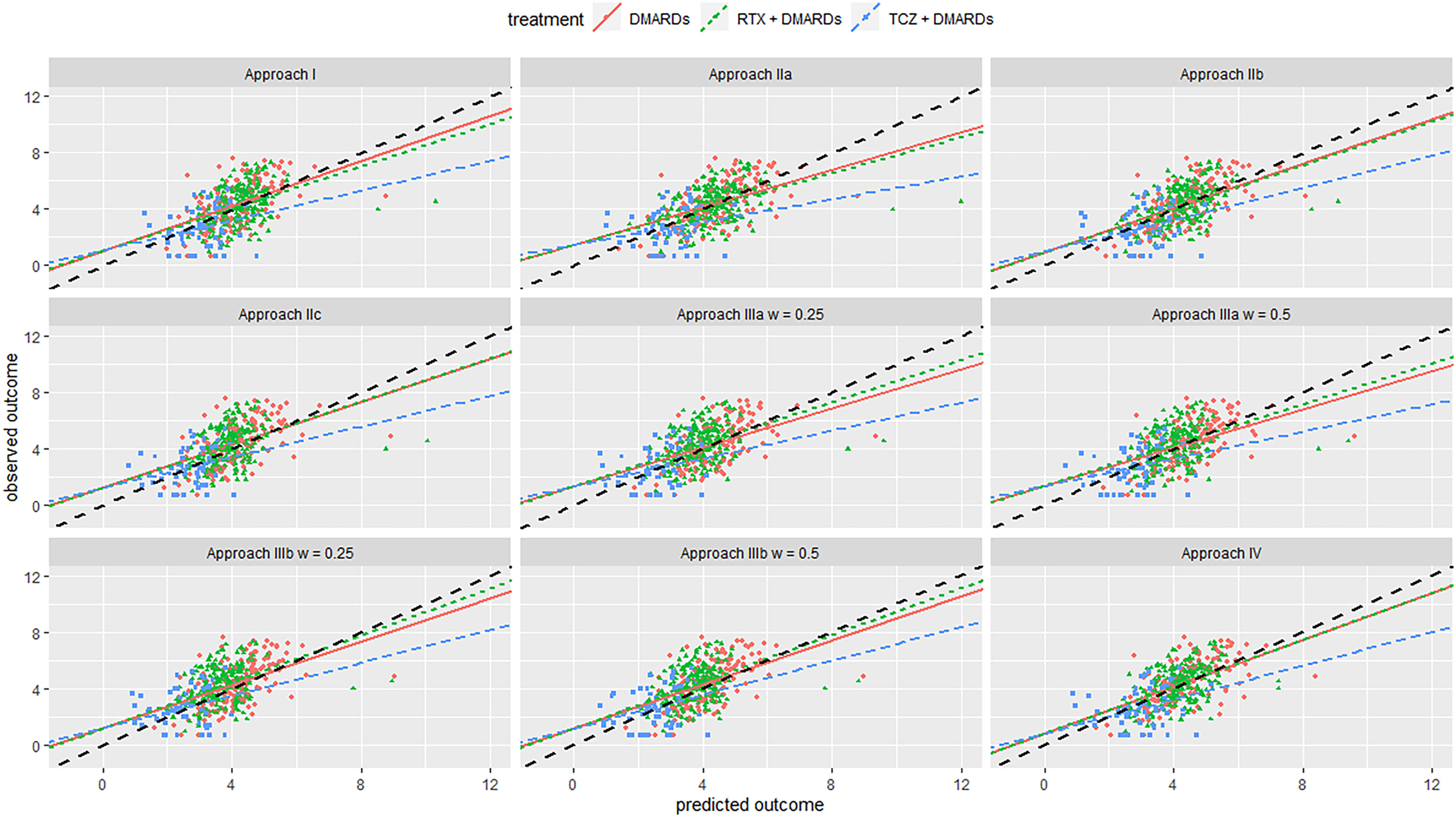
Calibration plot from internal–external validation, for the Swiss registry as the external data set. Black line is line of perfect calibration. Red line is the slope for DMARDs; green line is for RTX + DMARDs; blue line is for TCZ + DMARDs. Each dot represents one patient. Abbreviations: DMARDs: Disease-modifying anti-rheumatic drugs; RTX: rituximab; TCZ: tocilizumab.
Internal validation results of bias and MSE for different approaches.
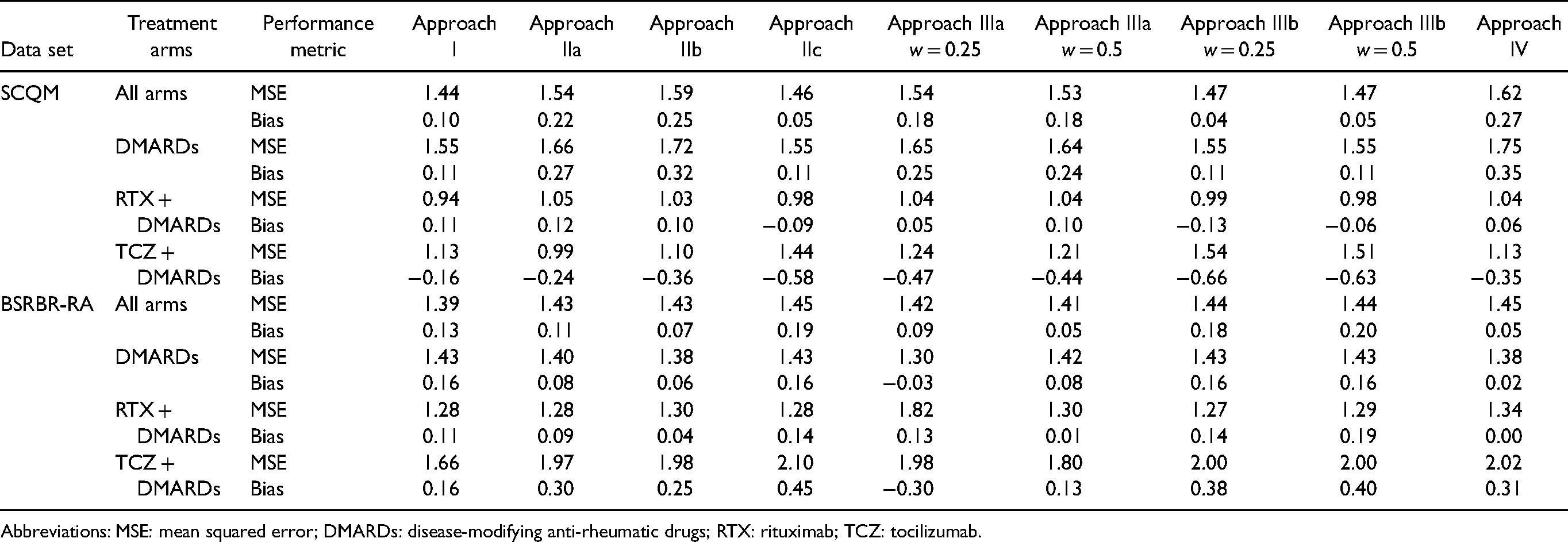
Abbreviations: MSE: mean squared error; DMARDs: disease-modifying anti-rheumatic drugs; RTX: rituximab; TCZ: tocilizumab.
Internal validation results of the calibration lines and R-squared for different approaches.
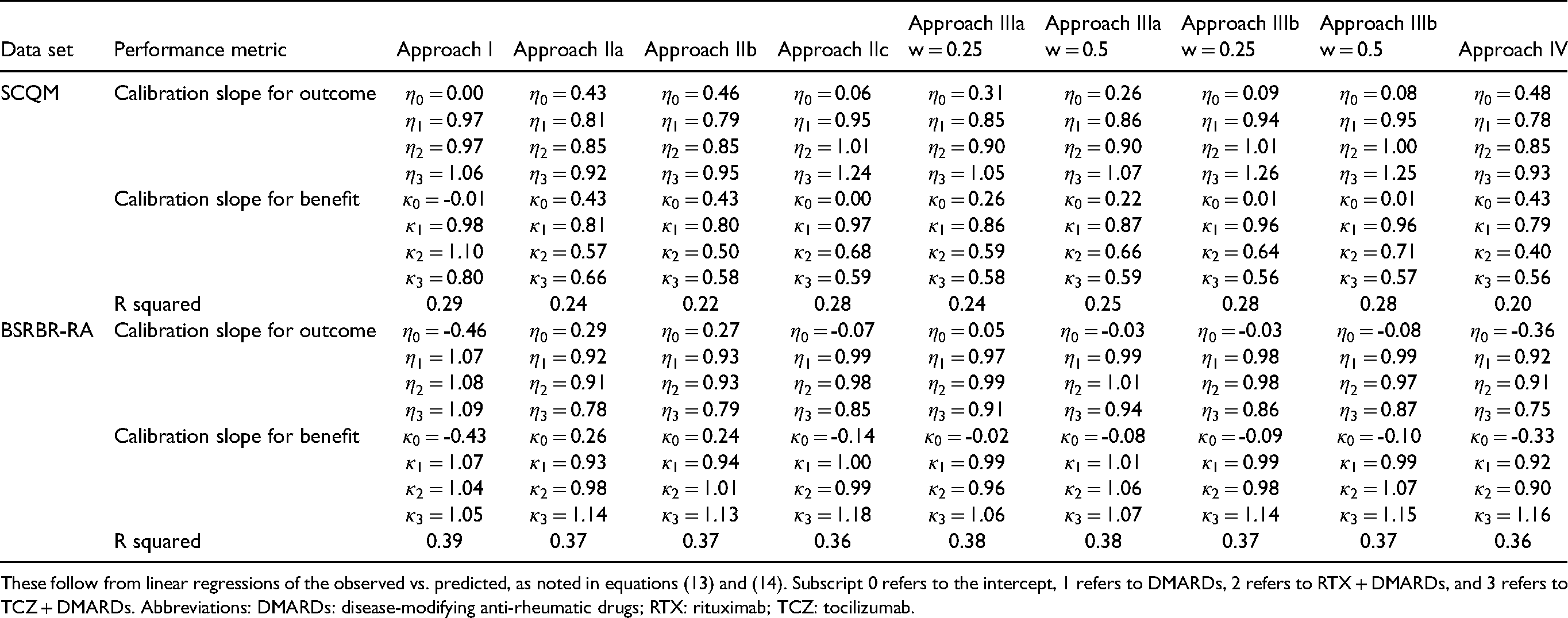
These follow from linear regressions of the observed vs. predicted, as noted in equations (13) and (14). Subscript 0 refers to the intercept, 1 refers to DMARDs, 2 refers to RTX + DMARDs, and 3 refers to TCZ + DMARDs. Abbreviations: DMARDs: disease-modifying anti-rheumatic drugs; RTX: rituximab; TCZ: tocilizumab.
Next, we discuss results from the internal–external validation. This procedure gave us some insight into the models’ expected performance when applied in new settings. Results are summarized in Tables 4, 5, and Figures 2, 3. Overall, calibration lines’ intercepts were far from zero for most models, and R-squared values were quite low, indicating low performance. Removing Swiss registry data from the training set and using it for validation resulted in models IIa, IIb, and IIIb performing best. Likewise, when we left the British registry out, we saw that model IIb and IV performed best Approaches IIb and IV gave almost the same results and were overall the best for both registries. They had the lowest overall MSE, relatively higher R-squared value and lower bias for all treatment arms and were slightly better calibrated for both the absolute outcome and treatment benefit compared to the other models. This showed that utilizing information from RCTs can help us better predict real-world outcomes compared to using only data from NRS. It also showed that in this data set there was little evidence of an effect modification. Thus, if we aim to make predictions about patients in a new setting (e.g. another country), for which no data are currently available, we would recommend Approaches IIb or IV. See also the Discussion section on additional considerations regarding generalizability.
Calibration plot from internal-external validation, for the British registry as the external data set. Black line is line of perfect calibration. Red line is slope for DMARDs; green line is for RTX + DMARDs; the blue line is for TCZ + DMARDs. Each dot represents one patient. Abbreviations: DMARDs: Disease-modifying anti-rheumatic drugs; RTX: rituximab; TCZ: tocilizumab.
Internal–external validation results for MSE and bias, for difference approaches.
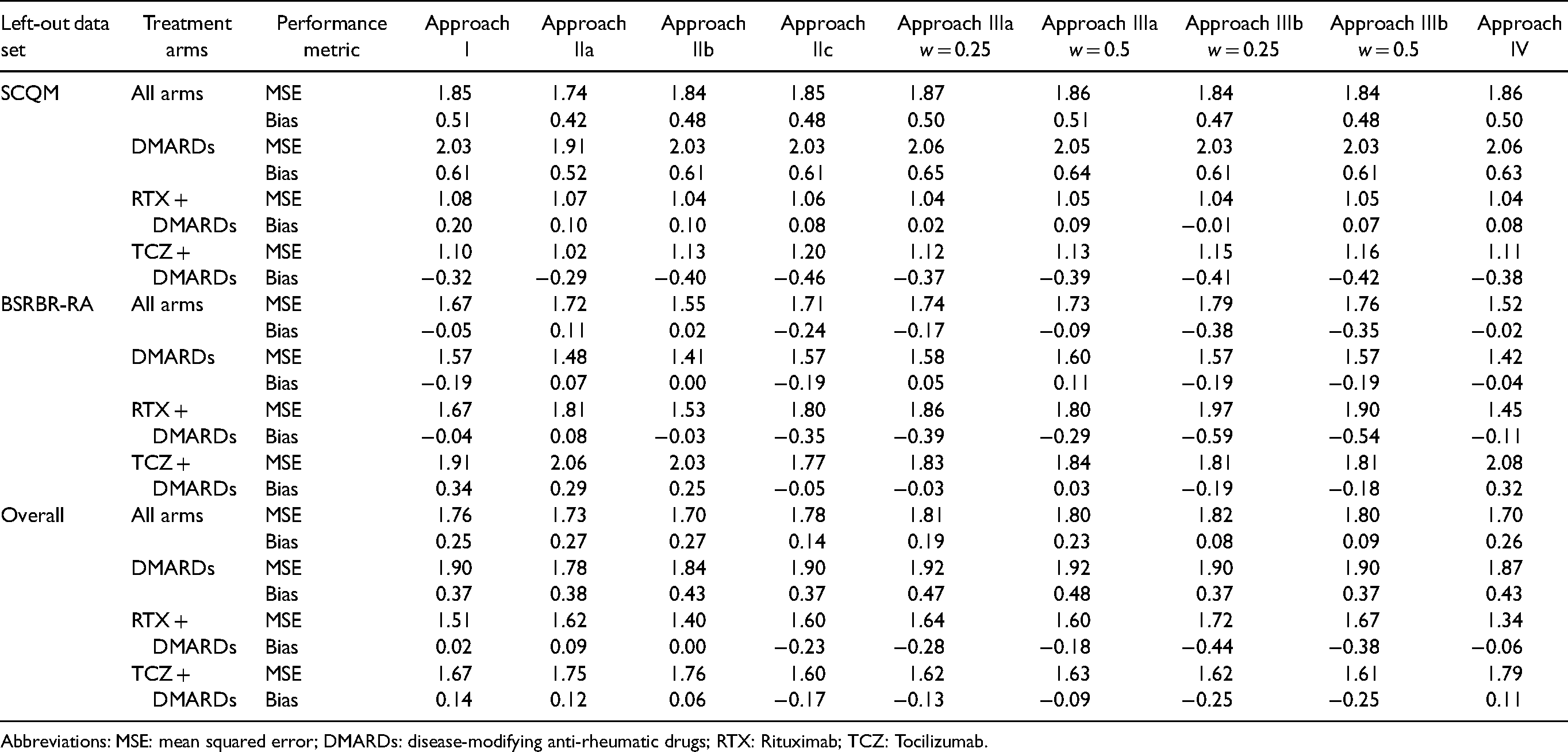
Abbreviations: MSE: mean squared error; DMARDs: disease-modifying anti-rheumatic drugs; RTX: Rituximab; TCZ: Tocilizumab.
Internal–external validation results of the calibration lines and R-squared for different approaches.
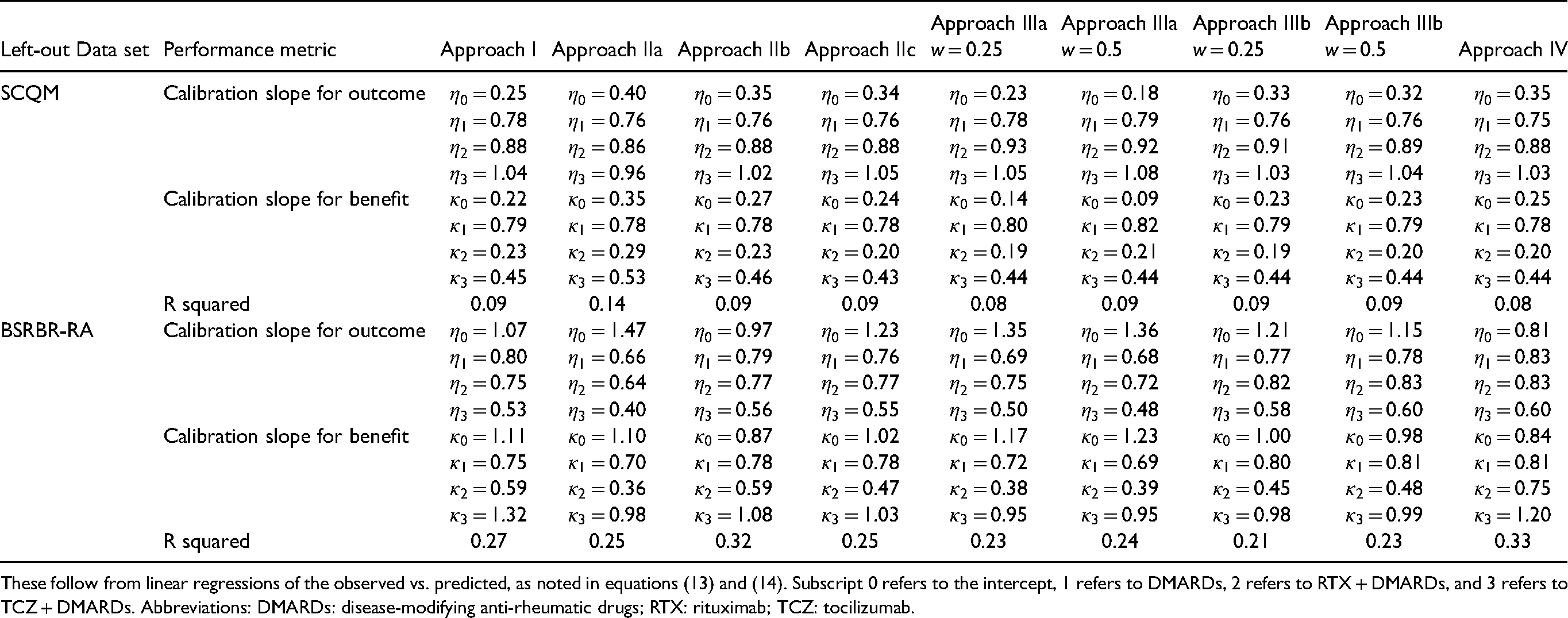
These follow from linear regressions of the observed vs. predicted, as noted in equations (13) and (14). Subscript 0 refers to the intercept, 1 refers to DMARDs, 2 refers to RTX + DMARDs, and 3 refers to TCZ + DMARDs. Abbreviations: DMARDs: disease-modifying anti-rheumatic drugs; RTX: rituximab; TCZ: tocilizumab.
Figure 4 summarizes the MSE and bias results for both internal and internal-external validation. In Table 9 of the Appendix we show results after correcting for optimism. We saw that Approach I had slightly larger optimism, as compared to other methods. However, these optimism-corrected results did not materially change the conclusion drawn from the main analyses. This is because optimism was generally quite small for all models. This was expected, since the sample size was big, the outcome was (approximately) continuous, and we only used few predictors. Finally, results did not materially change when using different prior distributions for .
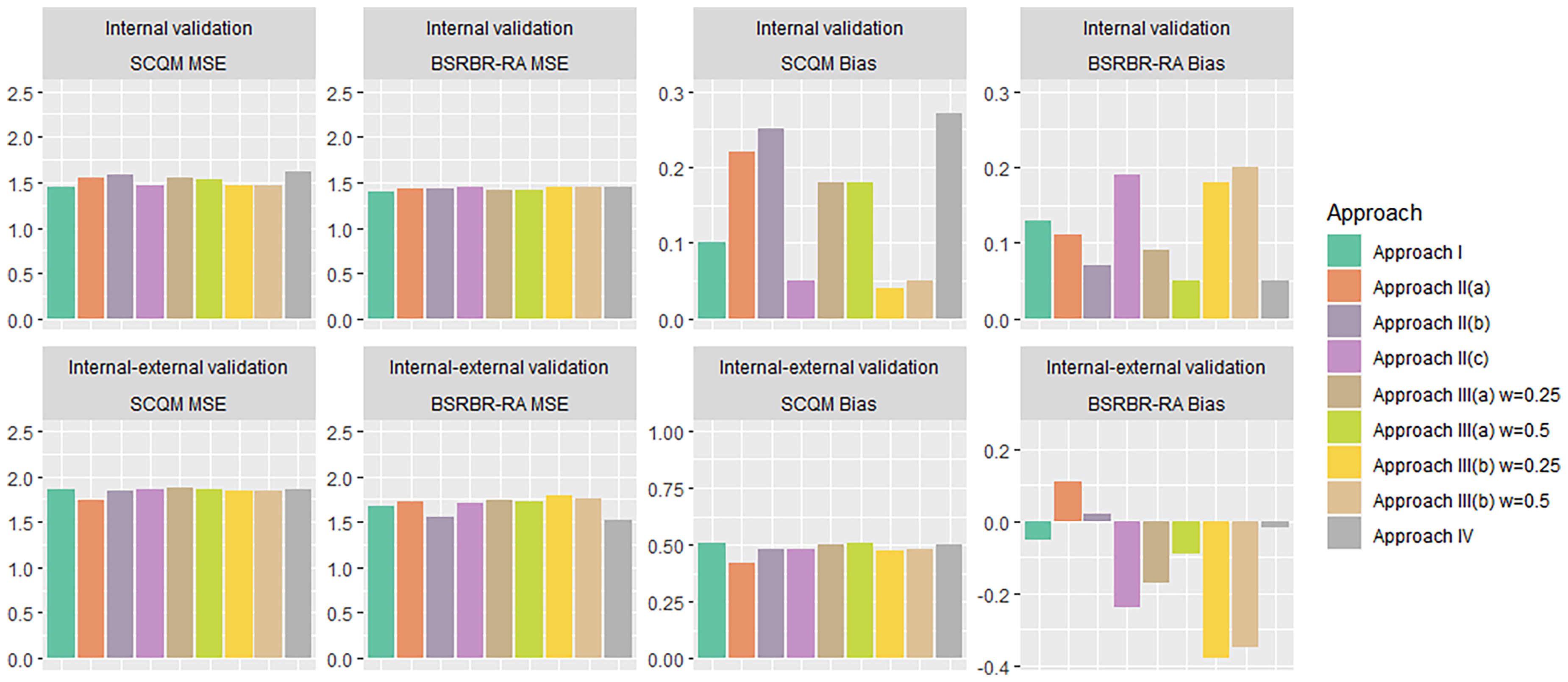
Bar plot summarizing MSE and bias calculated through an internal (top row) and internal–external (bottom row) validation, for the Swiss and British registry (SCQM and BSRBR-RA respectively). For internal–external validation, the labelled study is used as the target data set. Abbreviations: MSE: Mean squared error; DMARDs: Disease-modifying anti-rheumatic drugs; RTX: rituximab; TCZ: tocilizumab.
Discussion
This paper presents a general framework for developing methods to predict real-world outcomes for a range of different treatment options. We focussed on continuous outcomes and proposed various prediction modelling approaches and methods for assessing their performance. Our models were based on two-stage IPD NMA and utilized both randomized and observational data.
We used a data set of patients with RA obtained from three RCTs and two registries to illustrate our methods. For this example, we developed six meta-analytical models and a simpler model (i.e. Approach I). The latter only utilized data from a single registry at a time. After fitting each model, we assessed its internal and internal–external performance while adjusting for optimism. In these validations, we compared observed outcomes versus predictions for all registry patients and calculated bias, MSE, and R-squared. We also fitted calibration lines, both for the overall outcome as well as for treatment benefit.
For our example, internal validation showed that Approach I was among the best performing approaches for both the Swiss and the British registry. Thus, for this particular example, the incorporation of RCT data and advanced meta-analytical modelling brought small benefit in terms of predictive ability for patients found in these two registries. Conversely, the internal–external cross-validation procedure identified Approaches IIb and IV as the best-performing ones. This suggested that these two might be the best for patients found in a completely new setting among all developed models. However, we should keep in mind that to establish the generalizability of a model, we would need data from multiple real-world settings to be available. In case of important heterogeneity (i.e. when there are great differences across different real-world settings), it will be tough to make predictions about patients found in new settings. This is one general limitation of all proposed methods.
Another important limitation of our approach is the need for IPD from multiple sources. IPD is generally hard to obtain at the MA level. However, new initiatives have been recently launched, such as YODA (https://yoda.yale.edu/), Vivli (https://vivli.org/), and Clinical Study Data Request (https://www.clinicalstudydatarequestcom/), aiming to promote large-scale IPD sharing. Moreover, our approach requires a connected network of interventions. In practical applications, the available NRSs may not include all interventions of interest (despite forming a closed network). In such cases, although we can still use some of the described methods to make predictions for outcomes under the missing treatments, there is no way to assess the goodness of these predictions for these particular settings. Another limitation is that we only discussed the case of comparative studies, i.e. studies that included more than one treatment. A generalization of the methods to include single-arm studies might be of interest in a follow-up project.
An additional limitation is that the proposed linear model (with only two-way interactions between treatment and covariate) might be too simple to predict accurately in the real-world. If a non-linear relationship is suspected, we could consider models that include fractional polynomials or cubic splines. Alternative approaches include tree-based methods.40–42 However, we did not explore them in detail.
In Approach III, we used fixed weighting factors . We arbitrarily used values of 0.25 and 0.5 for these factors. Sensitivity analysis showed that using different values did not alter much the performance of the model. Alternatively, we could have used flexible weighting, e.g. by assigning a prior distribution to , treating the weight as a random variable. 15 This is similar to the ‘power prior’ approach.43,44 We fitted a model that used a modification of the power prior approach, called normalized power prior45,46 in the RA data set. In this model, the parameter estimates from NRS are down-weighted according to whether they agree with the RCT estimates. In the case of a large disagreement, there is more down-weighting. We found that the weighting factors decreased all the way down to zero for the RA data set, negating all information from the NRS. For large sample data sets the RCTs and NRS are likely to disagree (i.e. large discrepancies between the mean and variance of RCTs and NRS), which will lead to pronounced down-weighting. 47 Thus, we did not show models based on the power prior in this paper; however, this might be an interesting area for future development. Also, we could assign weights to different model parameters, e.g. the intercept term, if deemed appropriate; we did not pursue this further in this paper. Another limitation of our methods is that it may often be difficult to use calibration measures (i.e. calibration intercept and slope for predicted outcome and predicted benefit) to compare the performance between competing models. It is possible that some models yield accurate outcome predictions (i.e. prognosis) but not of treatment benefit, and vice versa. Selecting an appropriate model will then strongly depend on the context in which the model should be used.
Moreover, we could have explored approaches where penalization also applies to prognostic factors and not only to effect modifiers, and also other penalization methods. Also, we only discussed two-stage meta-analytical approaches; however, making these methods one-stage is straightforward. Another interesting idea suggested by one of our anonymous reviewers would be to include study design as yet another predictor in the second-stage model. However, it would be difficult to implement in our data set, which only includes two NRS; we leave this idea for future research.
In this paper, we used a simple regression adjustment for estimating treatment effects from the observational studies. Alternative methods such as propensity score matching 48 or inverse probability of treatment weighting (IPTW) could be used when the assumptions behind the regression adjustment seem implausible. We explored the use of IPTW and preliminary results showed a similar performance to the models based on regression adjustment. Thus, we decided to leave this for future work. Note, however, that no method for causal inference guarantees unbiased estimation of treatment effects from the observational studies. In our framework, when these estimates are biased, models that use this information (such as Approach IIa or IIb) are expected to perform worse, and thus not be selected at the end as the final model. Also, note that all methods for causal inference are limited by unmeasured confounding.
Furthermore, in practical applications, we often face the problem of ‘systematically missing’ predictors, i.e. when a predictor is missing for all individuals within particular studies in an IPD MA. There have been methods proposed for imputing such predictors, based on the missing at random assumption.
49
There is also an R package
Finally, we note that our methods need to be extended to cover the case of binary and time-to-event outcomes. This might be challenging, especially when assessing the predictive performance of different approaches using calibration for treatment benefit. For example, the so-called c-statistic for benefit was recently proposed 51 and might be used to this end; however, future research is needed to investigate this.
To summarize, this is the first paper to propose and compare two-stage meta-analytical IPD models for predicting the real-world effectiveness of interventions to the best of our knowledge. The gain in predictive performance from combining RCTs and NRS was modest in our clinical example. Nevertheless, the illustration of different modelling approaches and the considerations regarding different cross-validation methods that we provide may be valuable to inform future studies aiming to predict real-world outcomes of competing interventions.
Supplemental Material
sj-docx-1-smm-10.1177_09622802221090759 - Supplemental material for Combining individual patient data from randomized and non-randomized studies to predict real-world effectiveness of interventions
Supplemental material, sj-docx-1-smm-10.1177_09622802221090759 for Combining individual patient data from randomized and non-randomized studies to predict real-world effectiveness of interventions by Michael Seo, Thomas PA Debray, Yann Ruffieux, Sandro Gsteiger, Sylwia Bujkiewicz, Axel Finckh, Matthias Egger and Orestis Efthimiou in Statistical Methods in Medical Research
Footnotes
Acknowledgements
A list of rheumatology offices and hospitals that are contributing to the SCQM registries can be found on www.scqm.ch/institutions. The SCQM is financially supported by pharmaceutical industries and donors. A list of financial supporters can be found on ![]() . The author(s) would like to thank the British Society for Rheumatology for use of this data. The BSR Biologics Register in Rheumatoid Arthritis (BSRBR-RA) is a project owned and run by the BSR on behalf of its members. BSR would like to thanks its funders for their support, currently AbbVie, Amgen, Celltrion, Eli Lilly, Pfizer, Samsung, Sandoz and Sanofi, and in the past Merck, Roche, Swedish Orphan Biovitrum (SOBI) and UCB. This income finances a wholly separate contract between BSR and The University of Manchester to host the BSRBR-RA. All decisions concerning analyses, interpretation and publication are made autonomously of any industrial contribution. The BSRBR-RA would like to gratefully acknowledge the support of BSR members and the National Institute for Health Research, through the Comprehensive Local Research Networks at participating centres; The authors would like to thank F. Hoffmann-La Roche and Clinical Study Data Request (https://clinicalstudydatarequest.com/) for providing the trial data.
. The author(s) would like to thank the British Society for Rheumatology for use of this data. The BSR Biologics Register in Rheumatoid Arthritis (BSRBR-RA) is a project owned and run by the BSR on behalf of its members. BSR would like to thanks its funders for their support, currently AbbVie, Amgen, Celltrion, Eli Lilly, Pfizer, Samsung, Sandoz and Sanofi, and in the past Merck, Roche, Swedish Orphan Biovitrum (SOBI) and UCB. This income finances a wholly separate contract between BSR and The University of Manchester to host the BSRBR-RA. All decisions concerning analyses, interpretation and publication are made autonomously of any industrial contribution. The BSRBR-RA would like to gratefully acknowledge the support of BSR members and the National Institute for Health Research, through the Comprehensive Local Research Networks at participating centres; The authors would like to thank F. Hoffmann-La Roche and Clinical Study Data Request (https://clinicalstudydatarequest.com/) for providing the trial data.
Author Note
Orestis Efthimiou, Institute of Primary Health Care (BIHAM), University of Bern, Bern, Switzerland.
Declaration of conflicting interests
The authors declared no potential conflicts of interest with respect to the research, authorship, and/or publication of this article.
Funding
The authors disclosed receipt of the following financial support for the research, authorship, and/or publication of this article: MS and OE were supported by the Swiss National Science Foundation (Ambizione grant number 180083). ME was supported by special project funding (grant 17841) from the Swiss National Science Foundation. SB was supported by the Medical Research Council (grant no. MR/R025223/1). TD acknowledges financial support from the Netherlands Organization for Health Research and Development (grant 91617050), and the European Union's Horizon 2020 Research and Innovation Programme under ReCoDID Grant Agreement no. 825746. This project has received funding from the European Union’s Horizon 2020 research and innovation programme under ReCoDID grant agreement no. 825746.
Supplemental Material
Supplemental material for this article is available online.
References
Supplementary Material
Please find the following supplemental material available below.
For Open Access articles published under a Creative Commons License, all supplemental material carries the same license as the article it is associated with.
For non-Open Access articles published, all supplemental material carries a non-exclusive license, and permission requests for re-use of supplemental material or any part of supplemental material shall be sent directly to the copyright owner as specified in the copyright notice associated with the article.