
Abstract
Poisson regression can be challenging with sparse data, in particular with certain data constellations where maximum likelihood estimates of regression coefficients do not exist. This paper provides a comprehensive evaluation of methods that give finite regression coefficients when maximum likelihood estimates do not exist, including Firth’s general approach to bias reduction, exact conditional Poisson regression, and a Bayesian estimator using weakly informative priors that can be obtained via data augmentation. Furthermore, we include in our evaluation a new proposal for a modification of Firth’s approach, improving its performance for predictions without compromising its attractive bias-correcting properties for regression coefficients. We illustrate the issue of the nonexistence of maximum likelihood estimates with a dataset arising from the recent outbreak of COVID-19 and an example from implant dentistry. All methods are evaluated in a comprehensive simulation study under a variety of realistic scenarios, evaluating their performance for prediction and estimation. To conclude, while exact conditional Poisson regression may be confined to small data sets only, both the modification of Firth’s approach and the Bayesian estimator are universally applicable solutions with attractive properties for prediction and estimation. While the Bayesian method needs specification of prior variances for the regression coefficients, the modified Firth approach does not require any user input.
Keywords
Introduction
Poisson regression is widely used to model the distribution of count variables as functions of predictive covariates. This approach provides particular utility when accommodating differential follow-up times of study subjects, 1 as well as the modelling of ‘non-events’ or excess zeroes through so-called zero-inflated models. 2 As with other generalized linear models, such as logistic regression, Poisson regression can be especially challenging in the presence of rare events, making it more likely that particular covariate patterns in a given dataset result in the nonexistence of maximum likelihood (ML) estimates; for example, if no events are observed for one of two groups represented by a binary covariate. A necessary and sufficient condition for the nonexistence of ML estimates has been identified by Correia et al. 3 This problem of ‘separation’ has been studied extensively for logistic regression,4–7 but comparatively little is known about how various approaches perform when separation arises in Poisson modelling, such as the bias reduction method of Firth8,9 and (in special cases) conditional exact Poisson (EP) regression. 10 Bayesian alternatives, including the application of weakly informative priors for the distribution of the log relative risk, have likewise not been evaluated with regard to separation. Given the common use of Poisson regression, particularly for rare events and in other settings that are prone to separation, more definitive empirical studies are needed to assess the comparative performance of these modelling options. In particular, we need to better understand how various modelling choices impact the estimation of regression coefficients to ensure that analysts are confident in their predictions.
In this paper, we provide a more comprehensive evaluation of methods that provide finite estimates of regression coefficients when separation arises. We propose a modification of Firth’s approach to improving its performance for predictions, without compromising its attractive bias-correcting properties for regression coefficients. Furthermore, we include the conditional median unbiased estimator 11 as implemented in the software package LOGXACT 10 or in SAS’s PROC GENMOD and a Bayesian estimator using weakly informative priors in our evaluation. To provide context, we first illustrate the issue of separation for rare event data with a dataset arising from the recent outbreak of COVID-19. We subsequently provide a brief review of Poisson regression and describe proposed solutions to the problem of separation. We then summarize the results of a comprehensive simulation study to compare these options under a variety of realistic scenarios. We further illustrate their relative performance with an additional example.
Motivating example
During the outbreak of the coronavirus (COVID-19) in winter and spring 2020, employees of supermarkets, nursing homes, and hospitals were considered key professionals as they are in contact with many clients each day even under the lockdowns of public life that were imposed by many countries in that time. Many of their clients such as older adults or persons with chronic diseases were considered to be at high risk of a severe course of the disease if they got infected. At some point, the question arose if more stringent control of virus spread should be imposed on one of these groups, in particular, considering the unknown probability of asymptomatic infections. Therefore, on 28 March 2020, and 30 March 2020, a representative series of 1161 tests for the presence of an infection with the novel coronavirus (COVID-19) was performed in Austria among randomly selected asymptomatic employees of supermarkets, nursing homes, and hospitals. 12
The research question behind this series was how the risk of infection differs between employees of supermarkets, nursing homes, and hospitals. The question could be answered by Poisson regression to compute risk ratios, for example, comparing nursing homes and hospitals to supermarkets.
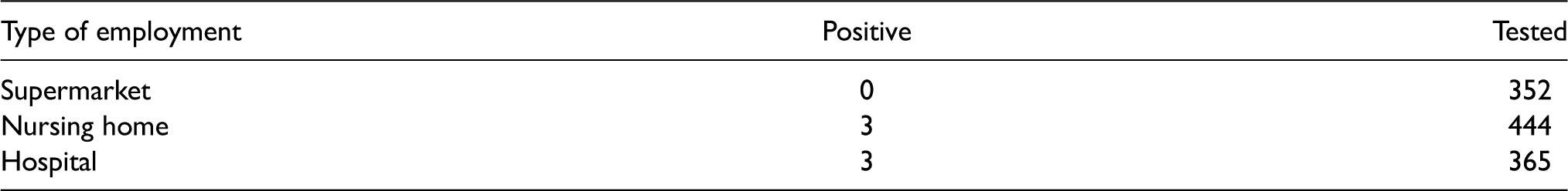
Among the 1161 persons tested, only six tested positive for COVID-19. Three of them were working in hospitals and three in nursing homes (Table 1).
Austrian COVID-19 test data.
Austrian COVID-19 test data.
Unfortunately, neither SAS/PROC GENMOD nor R/glm was able to provide risk ratios based on a Poisson regression analysis because ML analysis failed as there was a category with no events. However, the conditional median unbiased estimates for the two interesting risk ratios and associated exact 13 95% confidence intervals (CIs) were 3.05 (0.46, ∞) for nursing homes versus supermarkets and 3.71 (0.56, ∞) for hospitals versus supermarkets. Using Firth’s bias reduction approach, 8 which in the absence of covariates can be obtained by adding 0.5 events to each of the three observations, the analysis resulted in risk ratios (95% profile penalized likelihood (PPL) CI) of 5.55 (0.54, 746.13) and 6.75 (0.65, 907.60), respectively. Therefore, while it appears that employees of nursing homes or hospitals are at considerably higher risk of spreading the disease compared to supermarket employees, this claim is not fully supported by the study but still could be found in local media. Note that estimates of risk accompanied by 95% CI in each group, which could be obtained much easier than risk ratios, give a good summary of the data but do not answer the question of whether supermarket employees or health care workers are at higher risk of infection.
In this section, we will review the Poisson regression model with a special focus on nonexistence of ML estimates. We will further review Firth’s correction in the context of the Poisson regression model and we will propose a modification that gives unbiased predictions. Finally, we will present exact conditional analysis and Bayesian estimation with weakly informative priors.
The Poisson model
The Poisson model assumes that the counts of events in a study, Y, follow a Poisson distribution with parameter
The log-likelihood of the Poisson model is given by
Conditions for nonexistence of ML estimates in Poisson regression and consequences
In the coronavirus testing study, no infections were detected among the 352 supermarket workers, while among the 365 hospital employees, three were infected. The risk ratio would be computed as (3 of 365)/(0 of 352), which is not defined because of the division by zero. Similarly, there is no finite maximizer
As in logistic regression, adding covariates will not remove the nonexistence in Poisson regression. While numerical ML algorithms may declare convergence when the log-likelihood cannot be improved by a further iteration,
14
‘a spurious solution is characterized by a “perfect” fit for the observations with
Firth’s likelihood penalization applied to the Poisson model
Generally, Firth
8
suggested adding a penalty term to the log-likelihood of exponential family models that resembles the Jeffreys invariant prior such that the penalized log-likelihood becomes:
Already in Firth’s seminal paper,
8
an example with Poisson regression was included. However, Firth’s likelihood penalization (FL) for the Poisson model has not been studied any further. FL estimates maximizing (1) can be obtained through iteratively solving the modified score equations:
Similarly, in logistic regression with rare events, Firth’s penalization provides predicted probabilities that are on average higher than the observed event rate. To solve this problem, Puhr et al. 7 suggested two methods, ‘FL with intercept correction’ (FLIC) and ‘FL with added covariate’ (FLAC). Here we explore the performance of these methods in the setting of Poisson regression.
FLIC consists of first obtaining the FL solution and then to correct the intercept parameter by adding a constant
FLAC starts by estimating the FL solution as well, but this is only done to compute the values of
While the two approaches generally give different results for logistic regression, it is remarkable that not only the FLIC estimates, but also FLAC estimates of
Because FLIC and FLAC do not modify the FL regression coefficients, CI for the regression coefficients can be obtained out of the FL model, and in the case of data sparsity should preferably be computed by the PPL method.5,6 Here, a 
We have written a SAS macro FLACPOISSON that performs the Firth correction and the FLAC modification based on iterated data augmentation using repeated calls to PROC GENMOD (https://github.com/georgheinze/flicflac). For simplicity, we approximate the PPL CI in FLACPOISSON by evaluating the profile likelihood (PL) of the augmented data fixing the event counts of the pseudo data at the values
Alternative methods do deal with separation
Exact conditional Poisson regression with median unbiased estimation
In exact conditional Poisson regression, inference is based on the exact conditional likelihood of a parameter
Exact conditional Poisson regression does not provide an estimate of the intercept and thus cannot be used for prediction. The implementations in SAS/PROC GENMOD, in Cytel studio, and in Cytel’s PROC LOGXACT add-on for SAS 10 allow for computation of exact and mid-p CIs and more details can be found in the software documentation. 17 In the remainder, we will refer to this method as EP regression.
Bayesian data augmentation
Bayesian estimation with properly specified priors also solves the separation issue. To overcome problems of computing time and diagnostics in Bayesian analysis with Markov chain Monte Carlo algorithms, Sullivan and Greenland
18
illustrate the use of data augmentation to specify normal priors, including an example for Poisson regression. The spread of the normal prior for a regression coefficient is determined by the width of a prior interval for the associated IRR. For example, if a 95% prior interval for the IRR of (1/1000, 1000) is specified, then based on a normal distribution the prior standard error is
A simulation study
Methods
The methodology of our simulation study is described as recommended by Morris et al. 19
Covariates generated in the simulation study. I(x) is the indicator function that equals 1 if the argument x is true, and 0 otherwise. [x] indicates that the non-integer part of the argument x is eliminated.
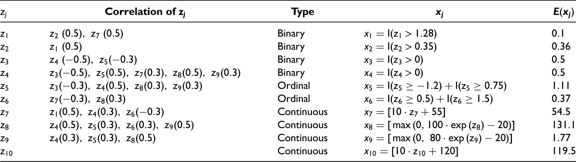
Covariates generated in the simulation study. I(x) is the indicator function that equals 1 if the argument x is true, and 0 otherwise. [x] indicates that the non-integer part of the argument x is eliminated.
To avoid extreme values for the two log-normally distributed covariates
We considered a full factorial design, varying the number of covariates,
We estimated 95% CI for regression coefficients by the Wald method for ML using PROC GENMOD, and by likelihood profiles applied to the augmented data for BDA, FL, and FLAC (FLACPOISSON macro). In the case of separation, the values for ML are those reported by PROC GENMOD at the last iteration.
Exact point and interval estimates and mid-p corrected CI were obtained by PROC LOGXACT. 10
Incidence of separation
The incidence of separation was generally higher in scenarios with smaller sample sizes and with larger negative values of
We only included EP in the comparison of methods for simulation scenarios with
Predictions
The description of the prediction performance is restricted to the methods ML, FL, FLAC, and BDA, since XL does not allow for predictions. Across all methods, predictions were more accurate in terms of RMSPE(
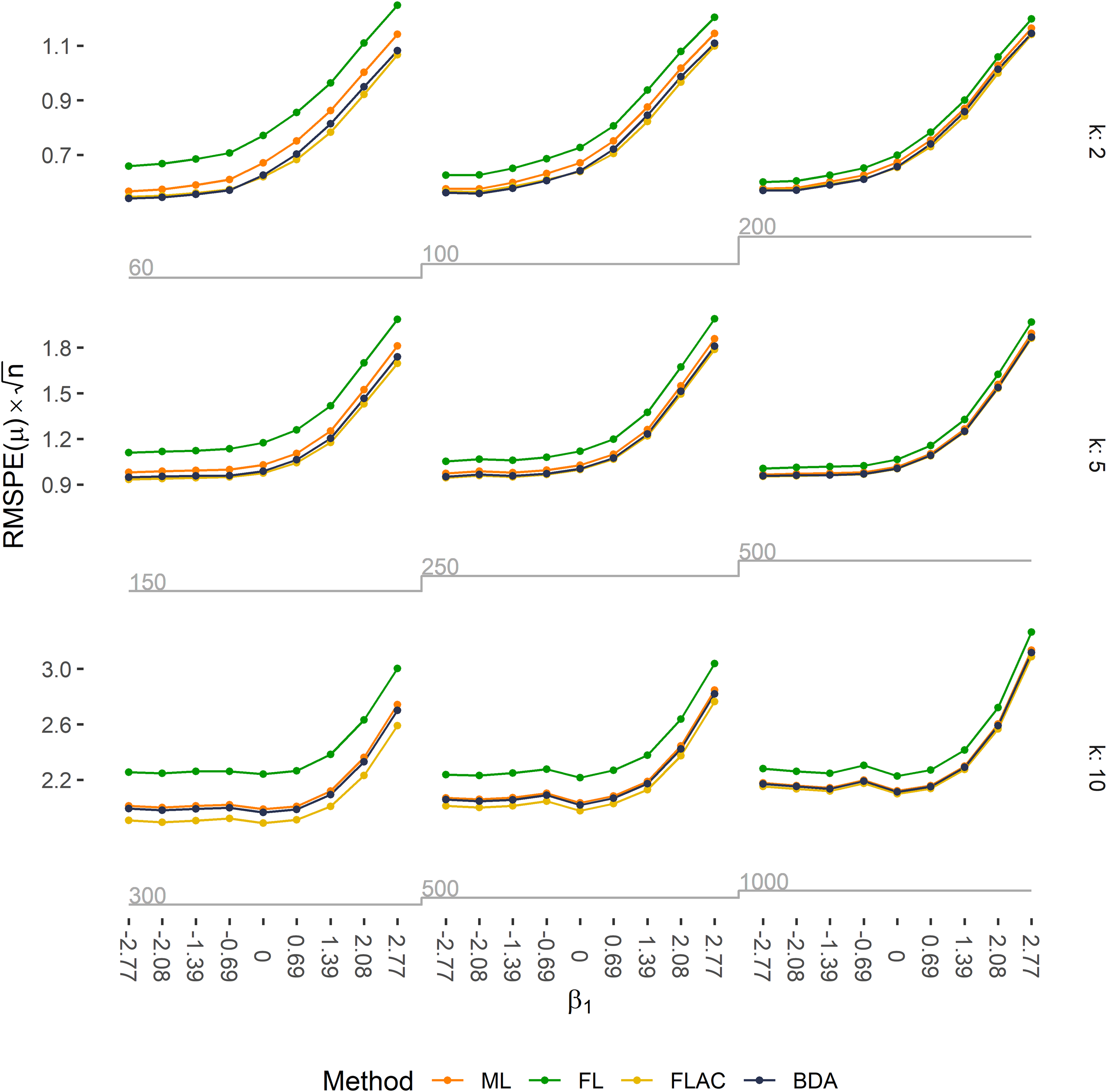
Predictive accuracy is expressed as RMSPE(μ) multiplied by the square root of the sample size n for all 81 simulation scenarios. Expected counts were obtained by ML, FL, FLAC, and BDA. Rows correspond to the number of covariates in the respective simulation scenario, columns to the EPV ratio, and ticks on the x-axis to the true value of
When
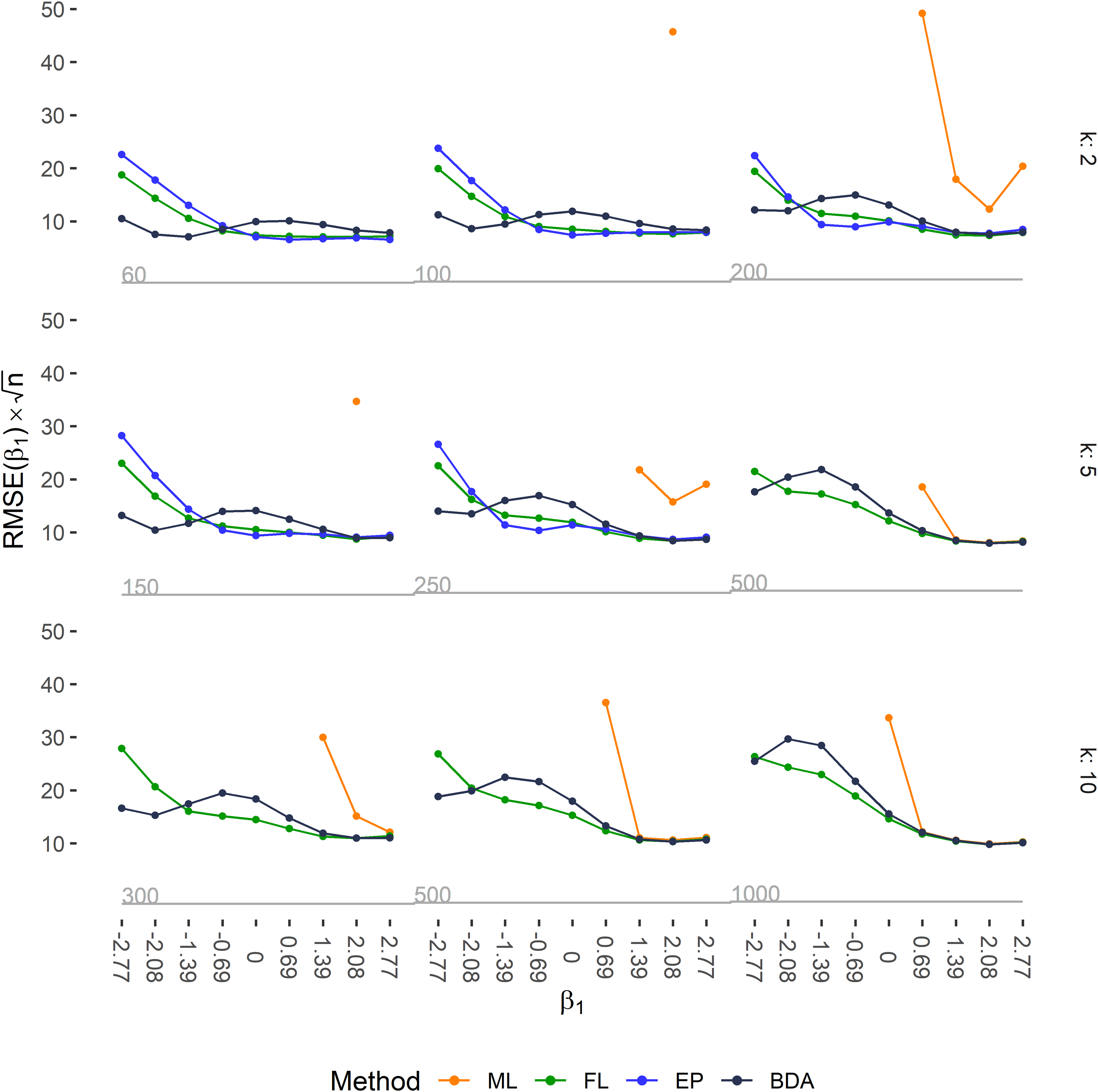
Accuracy of the estimated regression coefficient
ML lead to a large negative bias because of divergent estimation caused by separation when
Left-tailed and right-tailed coverage rates of 95% two-sided CIs are depicted in Figure 3, and the power to exclude
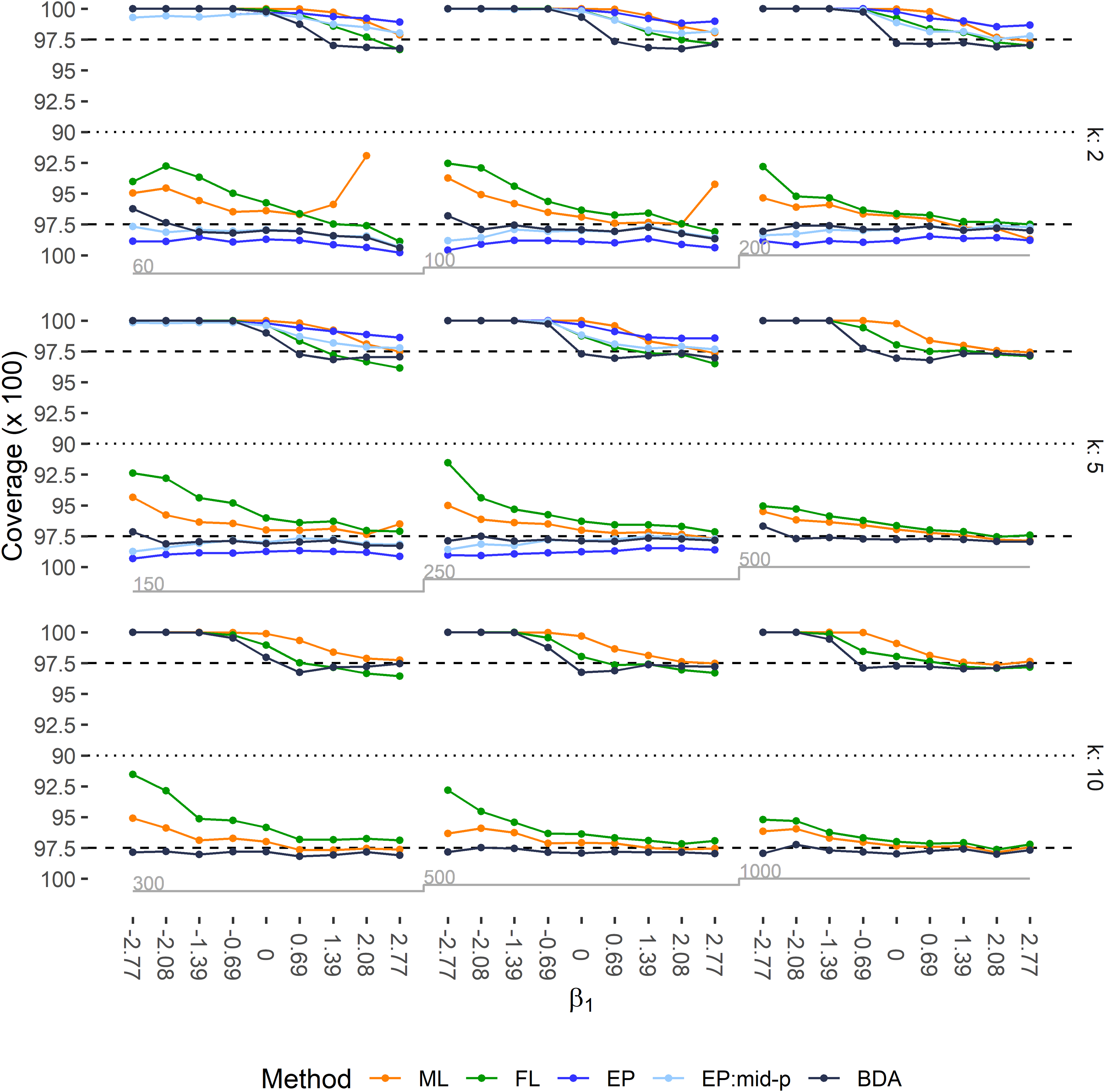
Left-tailed and right-tailed coverage of 95% two-sided CIs for regression coefficient
Feher et al. 25 studied risk factors for complications in implant dentistry. Risk factors were assessed in 1133 patients undergoing 2405 implantations. We used Poisson regression to model the number of haematological complications by the risk factors age (in decades), smoking (no smoking, light smoking, and heavy smoking), and diabetes mellitus and considered the number of implantations performed per patient as the rate multiplier. Smoking was coded using ‘ordinal coding’, that is, two dummy variables were defined contrasting light smokers from non-smokers, and heavy smokers from light smokers. Table S1 contains the basic descriptives for these variables.
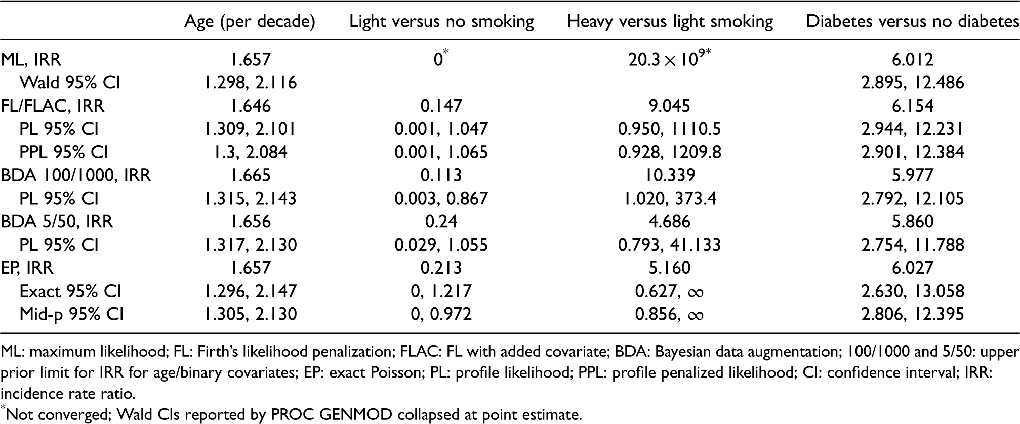
ML analysis failed to converge because no haematological complications were observed for light smokers (Table 3). This caused the regression coefficients of the two dummy variables associated with smoking to diverge. PROC GENMOD reported arbitrarily large estimates and standard errors for the corresponding regression coefficients but rather than reflecting the large standard errors, the reported Wald CI was collapsed at the point estimates.
Results for implant dentistry study: point estimates of IRRs and 95% CI.
Results for implant dentistry study: point estimates of IRRs and 95% CI.
ML: maximum likelihood; FL: Firth’s likelihood penalization; FLAC: FL with added covariate; BDA: Bayesian data augmentation; 100/1000 and 5/50: upper prior limit for IRR for age/binary covariates; EP: exact Poisson; PL: profile likelihood; PPL: profile penalized likelihood; CI: confidence interval; IRR: incidence rate ratio.
Not converged; Wald CIs reported by PROC GENMOD collapsed at point estimate.
By contrast, FL, BDA, and EP using the MUE gave plausible estimates for all variables (Table 3). These methods also supplied 95% CI, which provided some evidence that light smokers experienced fewer haematological complications than non-smokers or heavy smokers. When comparing the two methods of estimating CI for FL, as expected, fixing the pseudo data with weights computed at the maximum penalized likelihood estimate (‘PL CI’ from the augmented data, used in the simulation study) led to slightly narrower intervals than iterating the weights (‘PPL CI’). We also compared the impact of specifying different priors with BDA. Compared to weakly informative priors (‘BDA 100/1000’: 95% prior intervals for the IRR extending to 100 for age and to 1000 for the binary covariates, used in the simulation study), with narrower priors (‘BDA 5/50’: 95% prior intervals extending to 5 for age and to 50 for the binary covariates), all point estimates and nearly all CI were pulled towards unity. The effect of changing the prior was particularly strong for the two IRRs corresponding to smoking which caused the separation problem. Employing weakly informative priors resulted in CI supporting the hypothesis that light smokers experienced fewer complications than non-smokers and heavy smokers, while with narrower priors the CI included unity. EP generally resulted in IRR and CI closer to the estimates by BDA 5/50 than to the estimates by other methods.
While 37 hematologic complications were observed, 39.5 complications were predicted by FL, which estimated the intercept at −4.3728. Applying FLAC changed the intercept to −4.4382, and recalibrated the total number of predicted complications to the observed number of 37. Because age was centred at 50 years,
We proposed and investigated Poisson regression methods to deal with the problem of separation, which leads to nonexistence of ML estimates. We adapted two modifications of FL, namely FLIC and FLAC, which were originally developed to debias predictions in logistic regression, for Poisson regression. It turned out that in Poisson regression FLIC and FLAC lead to the same estimation method. This method, which we refer to as FLAC, competed well with alternative approaches such as EP regression, which needs special software and is only applicable for small-sized problems, or BDA, which is easy to implement but crucially depends on the choice of the width of the prior distribution. A possible advantage of BDA could arise if a model with many covariates should be fitted. It is essentially equal to ridge regression, and unlike FL can handle situations where the number of covariates exceeds the number of events by regularizing parameter estimates. In our application and simulations we fixed the variance of the prior distribution, which is inversely proportional to the penalty parameter in ridge regression. Optimizing that penalty parameter by, for example, cross-validation invalidates inference about regression coefficients, is not robust to separation 14 and can lead to instable results. 26 To sum up, for data sets fitting into the framework of this study, that is, with an EPV ratio of 3 or higher and moderate correlation between covariates, we advocate using FL as it does not need any user input or optimization of a penalty parameter and is computationally feasible, while showing good performance.
In some situations, count outcomes can be naturally reinterpreted as dichotomous outcomes, for example, in the coronavirus testing study where we can either count the number of infections per working place or determine whether a person is infected or not. These data allow for analysis via Poisson regression as well as via logistic regression. It was not the aim of this study to provide guidance on which analysis method to prefer with sparse data, but primarily the decision should depend on the estimand of interest, that is, whether risk ratios or odds ratios should be estimated. Our study employed a realistic design for simulations that resembled data one could typically see in epidemiological studies. Such a design is suitable to draw conclusions on the relative performance of methods in practically relevant situations. While in the simulation study we used R for data generation and summarizing results, we focused on the SAS software for fitting the Poisson models. SAS is widely used among epidemiologists, and with the Cytel SAS procedures, robust and efficient software was available to include EP regression in our comparisons. Hence we employed Cytel’s PROC LOGXACT for EP regression even if an implementation of EP regression is readily available in PROC GENMOD. We provide a SAS macro to apply the Firth correction and its modification FLAC in Poisson regression. The median unbiased estimator implemented in PROC LOGXACT has been described to suffer from extreme shrinkage in case the exact conditional distribution of the sufficient statistic is nearly degenerate. Therefore, an alternative estimator based on maximizing the conditional penalized likelihood was proposed. 27 We did not include it in our comparison as Heinze and Puhr 27 found it to be very similar to the FL estimator. We also did not consider the median bias-corrected estimator of Kosmidis et al. 28
R code for fitting a Poisson model with FL is also available, 29 however, without the possibility to invoke the FLAC extension or the estimation of PPL CI. We are also not aware of software packages in R which allow fitting EP regression models. Our SAS macro FLACPOISSON, a SAS macro to implement BDA and further SAS macros implementing FL and FLAC for logistic, conditional logistic and Cox regression are available on the GitHub repository https://github.com/georgheinze/flicflac. A further public repository, https://github.com/georgheinze/PoissonF, contains the aggregated data set of the implant dentistry study and code to reproduce its analysis, all codes used to conduct the simulation study, and an R markdown file which summarizes its results.
The FLAC method lends itself to several extensions. Most naturally, it can easily accommodate overdispersion by including the estimation of a dispersion parameter. 30 This can already be achieved with our SAS macro which is based on PROC GENMOD. Further work could be done to investigate the advantages of considering FLAC for this and other extensions, such as zero-inflated Poisson models and Poisson hurdle models.
Supplemental Material
sj-docx-1-smm-10.1177_09622802211065405 - Supplemental material for Solutions to problems of nonexistence of parameter estimates and sparse data bias in Poisson regression
Supplemental material, sj-docx-1-smm-10.1177_09622802211065405 for Solutions to problems of nonexistence of parameter estimates and sparse data bias in Poisson regression by Ashwini Joshi, Angelika Geroldinger, Lena Jiricka, Pralay Senchaudhuri, Christopher Corcoran and Georg Heinze in Statistical Methods in Medical Research
Footnotes
Acknowledgements
AJ acknowledges support by the research mobility grant (No. 331377) awarded by the Academy of Finland. AJ carried out parts of this work at Cytel Statistical Software and Services, Pune, India, and at Cytel Inc., Cambridge, MA, USA. PS and CC acknowledge the support by NIH, grant SBIR-9R44 GM104597-02A1. We thank Drs Kuchler, Gruber, and Feher from the University Clinic of Dentistry, Medical University of Vienna, for providing the data of the implant dentistry study which partly motivated this research.
Declaration of conflicting interests
The authors declared no potential conflicts of interest with respect to the research, authorship, and/or publication of this article.
Funding
The authors disclosed receipt of the following financial support for the research, authorship, and/or publication of this article: GH’s, AG’s, and LJ’s work were partly supported by the Austrian Science Fund (FWF), award I-2276-N33. AJ was supported by the research mobility grant (No. 331377) awarded by the Academy of Finland. PS and CC were supported by NIH, grant SBIR-9R44 GM104597-02A1.
Supplemental Material
Supplemental material for this article is available online.
Appendix 1
References
Supplementary Material
Please find the following supplemental material available below.
For Open Access articles published under a Creative Commons License, all supplemental material carries the same license as the article it is associated with.
For non-Open Access articles published, all supplemental material carries a non-exclusive license, and permission requests for re-use of supplemental material or any part of supplemental material shall be sent directly to the copyright owner as specified in the copyright notice associated with the article.