
Abstract
Background
The change in estimate is a popular approach for selecting confounders in epidemiology. It is recommended in epidemiologic textbooks and articles over significance test of coefficients, but concerns have been raised concerning its validity. Few simulation studies have been conducted to investigate its performance.
Methods
An extensive simulation study was realized to compare different implementations of the change in estimate method. The implementations were also compared when estimating the association of body mass index with diastolic blood pressure in the PROspective Québec Study on Work and Health.
Results
All methods were susceptible to introduce important bias and to produce confidence intervals that included the true effect much less often than expected in at least some scenarios. Overall mixed results were obtained regarding the accuracy of estimators, as measured by the mean squared error. No implementation adequately differentiated confounders from non-confounders. In the real data analysis, none of the implementation decreased the estimated standard error.
Conclusion
Based on these results, it is questionable whether change in estimate methods are beneficial in general, considering their low ability to improve the precision of estimates without introducing bias and inability to yield valid confidence intervals or to identify true confounders.
1 Background
Adjustment for potential confounders is routinely performed in etiological studies based on observational data. Subject matter expertise plays a pivotal role in identifying confounders. However, uncertainty often persists regarding whether some covariates are truly confounders or not. In a recent review of studies published in four major epidemiologic journals, only 146/292 (50%) of explicative studies indicated choosing adjustment covariates based on prior knowledge, and 30/146 (20%) of these reported also using data-driven methods. 1 In total, 69/292 (24%) of explicative studies reported using some data driven method to help selecting covariates. 1 This likely underestimates the prevalence of data-driven variable selection since 107/292 (37%) of studies did not provide sufficient information to determine how variables were selected. As such, variable selection based on the observed data is frequently attempted in epidemiology.
Also according to this review, the change in estimate (CIE) would be the most popular data-driven method for selecting confounders in epidemiologic studies. 1 Indeed, 34/69 (42%) of studies that used data-driven methods employed the CIE. Studies of varied size and fields of epidemiology were using the CIE. This is unsurprising considering that the CIE is recommended both in modern epidemiologic textbooks and articles over confounder selection methods based on P values in situations where the analyst determines that data-driven selection is warranted (see literature 2 , 3 and references therein). For example, in Chapter 15 of the 3rd edition of Modern Epidemiology, it is written “Although many have argued against the practice […], one often sees statistical tests used to select confounders (as in stepwise regression), rather than the change-in-estimate criterion just discussed.” 3
The most typical implementation of the CIE first entails fitting an outcome model according to the exposure and adjusted for all potential confounders. Potential confounders are then removed from the outcome model one at a time. The procedure stops once it becomes impossible to remove a potential confounder without altering too much the exposure effect estimate as compared to the estimate produced by the initial fully adjusted model. Intuitively, if all confounders are available, the fully adjusted model should yield an estimate that is appropriately adjusted for confounding. Any reduced model that yields an estimate similar to that of the fully adjusted model is thus also expected to provide adequate adjustment for confounding.
While the CIE is appealing because it is intuitive and simple to implement, concerns have been raised concerning its validity. For instance, it has been noted that the change in the effect estimate may partly reflect non-collapsibility instead of confounding when employing effect measures such as the odds ratio or the hazard ratio.2,4–6 A further critique of the CIE is that it is susceptible to produce invalid P values and confidence intervals. 3 This is because P values and confidence intervals are typically computed by statistical software assuming that the model is known a priori. When the model is selected based on the observed data, this assumption no longer holds. Finally, if the CIE is applied without reflecting on how covariates are causally related to the exposure and the outcome, it may lead to inappropriately controlling for colliders, thus introducing bias. 4
We are aware of only three simulation studies that have investigated the performance of the CIE.7–9 According to their results, the CIE would yield estimators with small bias and valid confidence intervals when a low change in estimate threshold is used (for example, 10%), but would fail to produce estimators with improved precision as compared to a model adjusting for all potential confounders. However, these simulation studies have a number of limitations. First, they consider scenarios with at most nine potential confounders.7–9 As such, situations with multiple potential confounders have never been investigated. Such situations are those where benefits from performing confounder selection are most expected. 2 Moreover, the CIE can be implemented in multiple ways. For example, in addition to the backward exclusion described earlier, it is also possible to proceed by forward inclusion of confounders. Forward implementation of the CIE is being used in practice, 1 but its performance has never been investigated as far as we know. Simulation studies have also focused on odds ratio effect measures. To the best of our knowledge, the performance of the CIE with hazard ratios or mean differences has never been examined.
The goal of the current study is thus to provide additional information regarding the performance of the CIE. We do not consider the problems caused by including colliders in the potential confounder set since it has already been shown that is impossible to distinguish between a confounder and a collider from the data alone.4,10 Hence, it is expected that the CIE would perform poorly when colliders are included among the potential confounders. Substantive knowledge input is essential for constructing the initial potential confounder set.
We have first conducted an extensive simulation study to investigate and compare the performance of various implementations of the CIE in a wide range of scenarios. Next, we compared the CIE implementations in a real data setting. This illustration, based on data from the PROspective Québec (PROQ) Study on Work and Health led by Brisson, 11 concerns the association between body mass index and diastolic blood pressure.
2 Simulation study
2.1 Simulation scenarios
The scenarios we have considered were inspired by the fourth data-generating process in Talbot et al.,
12
but feature more covariates. Let L1, L2, …, L30 represent a set of 30 potential confounders, X the exposure of interest and Y the outcome. For all scenarios, we have first simulated L6, L7, …, L30 as correlated normal variables with mean = 0, variance = 1, and correlations =
We have considered scenarios where Y was a continuous, binary, or time to event variable. When Y was continuous, it was generated as a normal variable with mean = 0.1L1 + 0.1 L2 + ⋯ + 0.1 L10 + βX and variance = 1. When Y was binary,
A causal diagram representing the relationships between the variables is presented in Figure 1. If this diagram was known to the investigator, confounder selection could be performed by ensuring that all backdoor paths from X to Y are blocked (see the appendix of VanderWeele and Shpitser
13
for an introduction to causal diagrams). For instance, adjusting for either
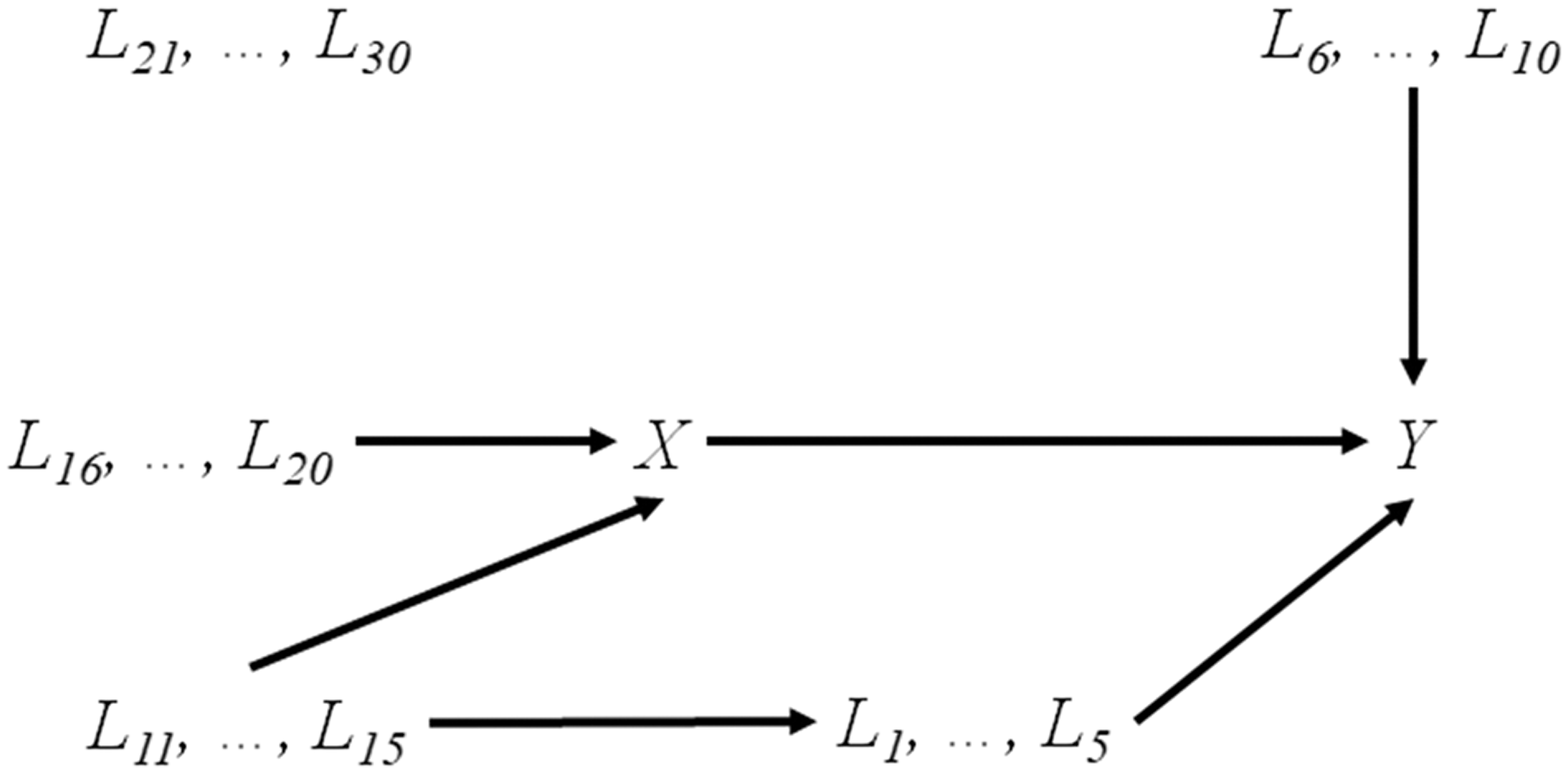
Causal diagram depicting the relationships between the variables in the simulation study. Arrows between groups of variables indicate that each variable of one group is causally affecting each variable in the second group. Variables L6, …, L30 are correlated in some scenarios (due to external/unobserved common causes).
A total of 54 different simulation scenarios were constructed by considering all possible combinations of the following factors: (1) sample size of n = 500 or n = 1000, (2) correlations
2.2 Change in estimate implementations
We have considered six different implementations of the CIE. These six implementations are first described generally, then details specific to the type of outcome are presented.
Backward – standard (BS). We have first fitted a model for the outcome according to the exposure and all covariates, and computed the effect estimate from this model. All covariates were then considered for exclusion, one at a time, and the relative difference in the effect estimate between the fully adjusted model and the model with one fewer variable was computed. The covariate whose exclusion altered the least the effect estimate was effectively excluded from the model. This process was repeated until it was impossible to exclude a covariate without changing the estimate by more than a pre-specified threshold as compared to the estimate from the fully adjusted model.
Backward – P values (BP). This implementation only differs from BS in that the covariate to be excluded at each step was the one whose associated P value was the largest.
Backward – confidence intervals (BC). We have started by fitting a model for the outcome according to the exposure and all potential confounders and determined the lower and upper bounds of the 95% confidence interval for the effect estimate. Next, covariates were considered for exclusion, one at a time. For each candidate, we calculated the relative change in each bound of the effect estimate’s confidence interval following the exclusion of the covariate and computed the maximum of these two changes. The covariate whose exclusion altered the least both bounds – the one with the smallest maximum change in bounds – was effectively excluded. This exclusion procedure was repeated until the maximum change in bounds of all candidates for exclusion was larger than a pre-specified threshold, comparing to the bounds of the fully adjusted model. Some authors have proposed that such an implementation may be superior to those focusing on estimates, because the confidence interval is usually the final product of an analysis. 3
Backward – mean squared error (BM). Again, a model for the outcome according to the exposure and all potential confounders was first fitted. The exposure coefficient and its estimated standard error are computed. The mean squared error (MSE) of this initial model is estimated as the square of the exposure coefficient’s standard error. Then, covariates are considered for exclusion, one at a time. For each candidate, we computed the estimated MSE as the square of the difference between the exposure coefficient from the reduced model and that of the initial model, plus the square of the exposure coefficient’s standard error in the reduced model. The covariate whose exclusion yielded the lowest estimated MSE was effectively excluded. The exclusion procedure stopped once excluding any of the candidates for exclusion increased the estimated MSE as compared to the one in the previous step. This is a slightly adapted version of the procedure proposed by Greenland et al., 14 which is designed to focus on accurate exposure effect estimation, as measured by the MSE.
Forward – crude (FC). We have first fitted a model for the outcome according to the exposure only and calculated the exposure effect estimate. All covariates were then considered for inclusion, one at a time. The covariate whose inclusion altered the most the estimate was effectively included. The estimate from the model adjusting for one additional covariate became the new comparator. This inclusion process was repeated until all candidates for inclusion altered the effect estimate by less than a pre-specified threshold.
Forward – partial (FP). This implementation only differs from FC in that the initial model was adjusted for L1, L2, L3, L6, L7. This implementation seeks to imitate a situation where the investigator is able to identify some confounders and risk factors of the outcome based on prior knowledge but is unsure about the status of the other potential confounders.
For all implementations, the model was a linear regression when Y was continuous, a logistic regression when Y was binary, and a Cox regression when Y was a time to event. For all implementations, except BM, the exposure effect estimate for determining the change in estimate was a mean difference, an odds ratio or a hazard ratio, when Y was continuous, binary or a time to event, respectively. For BM, the change in MSE was based on the regression coefficient, regardless of the type of outcome. Three different changes in estimate thresholds were used for each implementation, except BM: 1%, 5% and 10%. For BM, there was no threshold. Percentages following implementation abbreviations are henceforth used to indicate the threshold.
2.3 Analysis
For each scenario, 1000 datasets were generated. The exposure effect was estimated with each of the 16 combinations of CIE implementation and threshold value, as well as with an unadjusted model and a fully adjusted model. For each of these 18 analysis methods (16 CIE implementations, unadjusted model and fully adjusted model), we first computed bias as the difference between the estimated exposure coefficient and the true exposure effect coefficient. For scenarios with a continuous outcome, this true exposure coefficient is the value of
3 Results
The Monte Carlo standard error was less than 0.008 for estimating bias, 0.006 for estimating standard error, and 0.016 for estimating coverage.
16
The results did not vary much according to sample size and amount of correlation between covariates. Therefore, only tables presenting the results for n = 500 and
3.1 Continuous outcome
Table 1 and Web Tables 1–5 summarize the results of the scenarios with a continuous outcome. When
Results of scenarios with continuous outcome, n = 500 and ρ = 0.2.
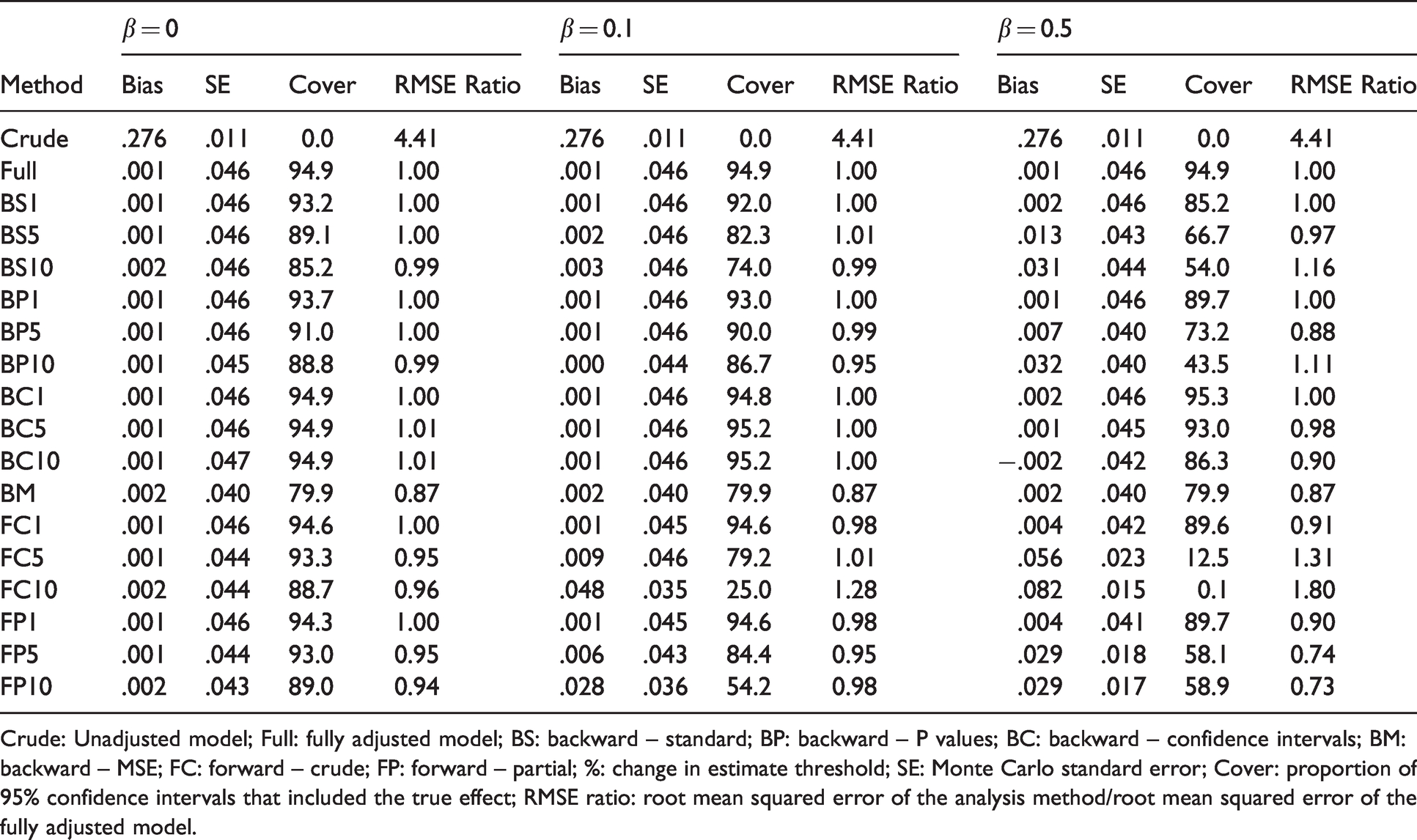
Crude: Unadjusted model; Full: fully adjusted model; BS: backward – standard; BP: backward – P values; BC: backward – confidence intervals; BM: backward – MSE; FC: forward – crude; FP: forward – partial; %: change in estimate threshold; SE: Monte Carlo standard error; Cover: proportion of 95% confidence intervals that included the true effect; RMSE ratio: root mean squared error of the analysis method/root mean squared error of the fully adjusted model.
Results of scenarios with binary outcome, n = 500 and ρ = 0.2.
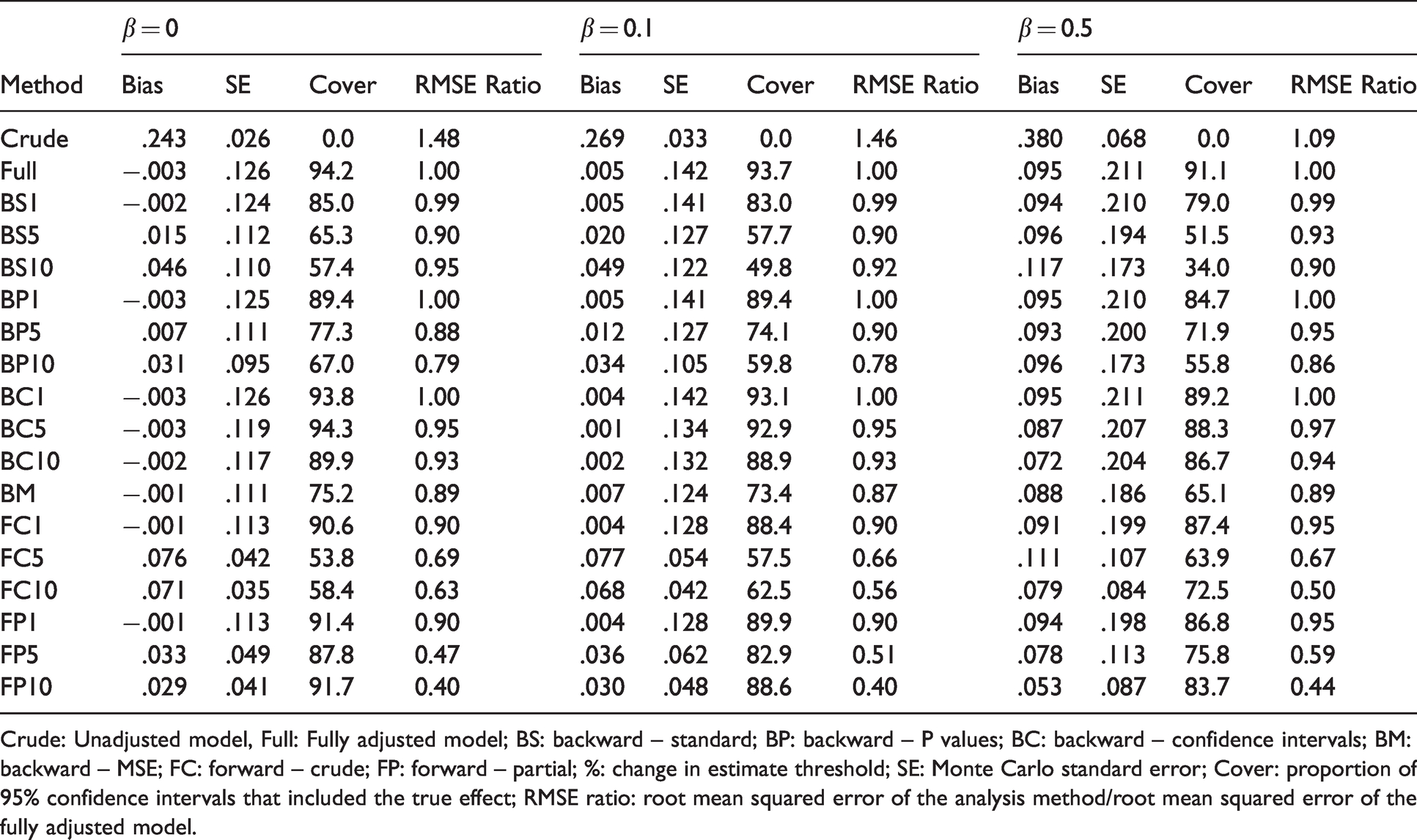
Crude: Unadjusted model, Full: Fully adjusted model; BS: backward – standard; BP: backward – P values; BC: backward – confidence intervals; BM: backward – MSE; FC: forward – crude; FP: forward – partial; %: change in estimate threshold; SE: Monte Carlo standard error; Cover: proportion of 95% confidence intervals that included the true effect; RMSE ratio: root mean squared error of the analysis method/root mean squared error of the fully adjusted model.
Results of scenarios with time to event outcome, n = 500 and ρ = 0.2.
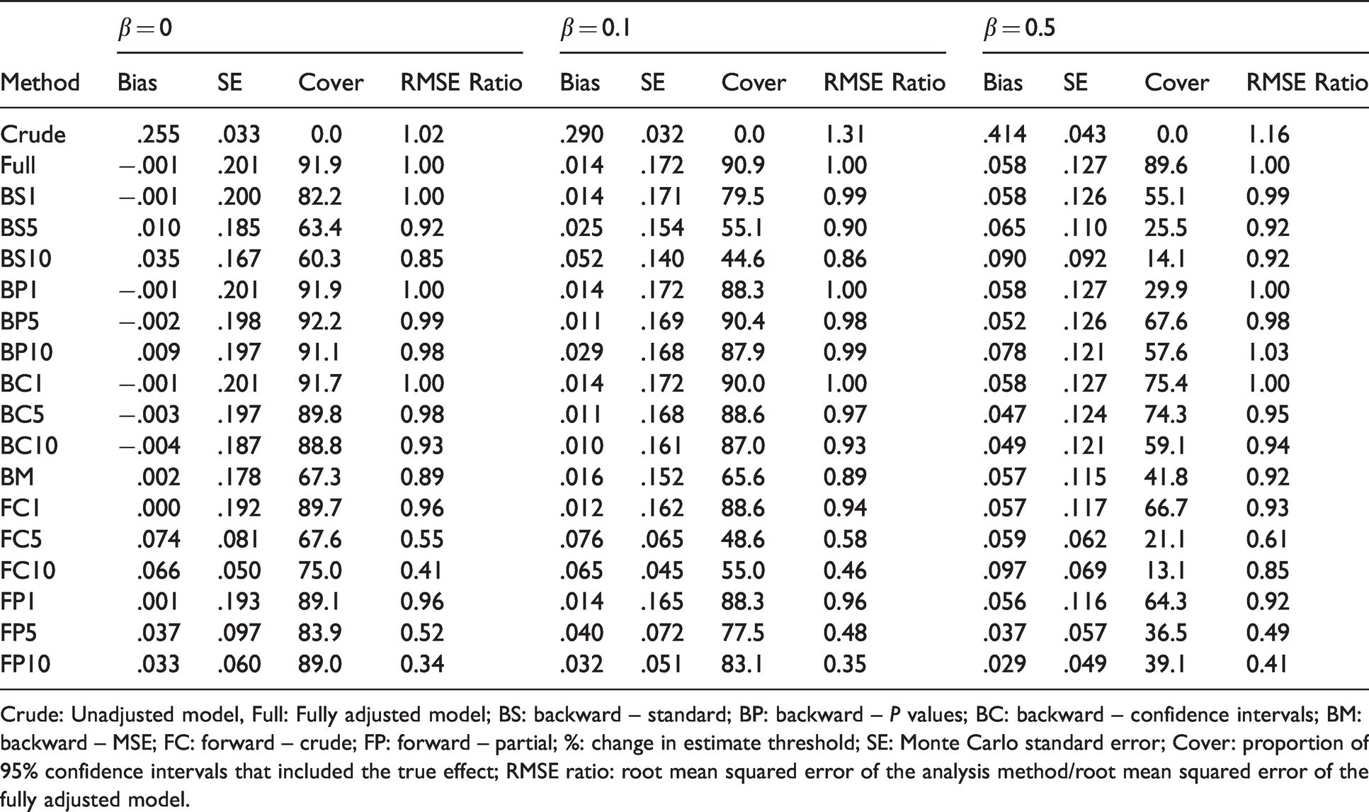
Crude: Unadjusted model, Full: Fully adjusted model; BS: backward – standard; BP: backward – P values; BC: backward – confidence intervals; BM: backward – MSE; FC: forward – crude; FP: forward – partial; %: change in estimate threshold; SE: Monte Carlo standard error; Cover: proportion of 95% confidence intervals that included the true effect; RMSE ratio: root mean squared error of the analysis method/root mean squared error of the fully adjusted model.
Proportion of simulation replicates in which a set sufficient to control confounding (S) was selected and average proportion of inclusion of each instrument (I) and other variable (O).
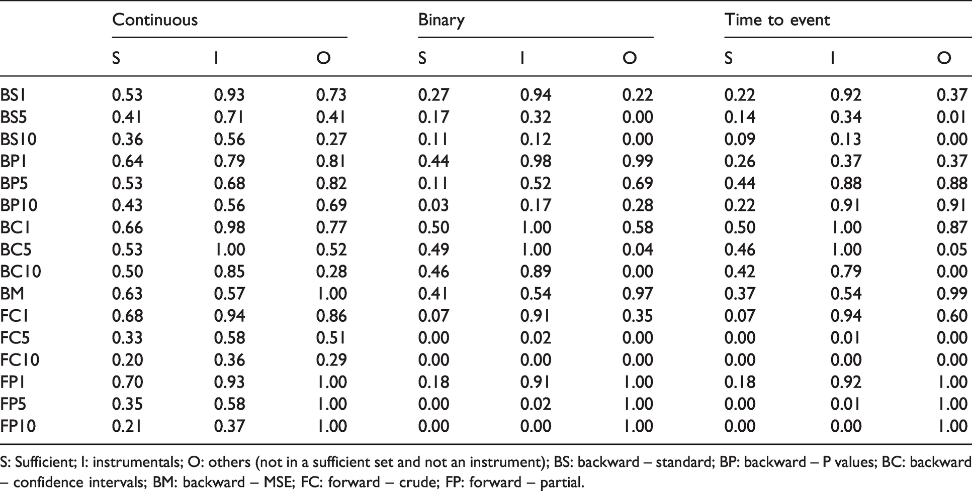
S: Sufficient; I: instrumentals; O: others (not in a sufficient set and not an instrument); BS: backward – standard; BP: backward – P values; BC: backward – confidence intervals; BM: backward – MSE; FC: forward – crude; FP: forward – partial.
Characteristics of the extracted sample from the PROspective Québec (PROQ) Study on Work and Health according to body mass index.
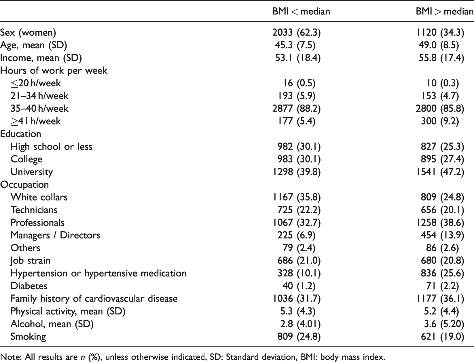
Note: All results are n (%), unless otherwise indicated, SD: Standard deviation, BMI: body mass index.
All CIE implementations produced confidence intervals that included the true effect in less than 90% of replications in at least some scenarios, except for BC1% and BC5%. Overall, the coverage of confidence intervals tended to be lower when the true effect increased, when a larger threshold was used or for the larger sample size. Forward implementations generally had confidence intervals with the lowest coverage, sometimes as low as 0%.
Only the BM implementation achieved a modest RMSE reduction as compared to the fully adjusted model, around 10%, in all scenarios. When
3.2 Binary outcome
The results for the scenarios with a binary outcome are presented in Table 2 and Web Tables 6–10. When
Estimate and selected covariates for the association between body mass index and diastolic blood pressure in the PROspective Québec (PROQ) Study on Work and Health according to change-in-estimate implementation.
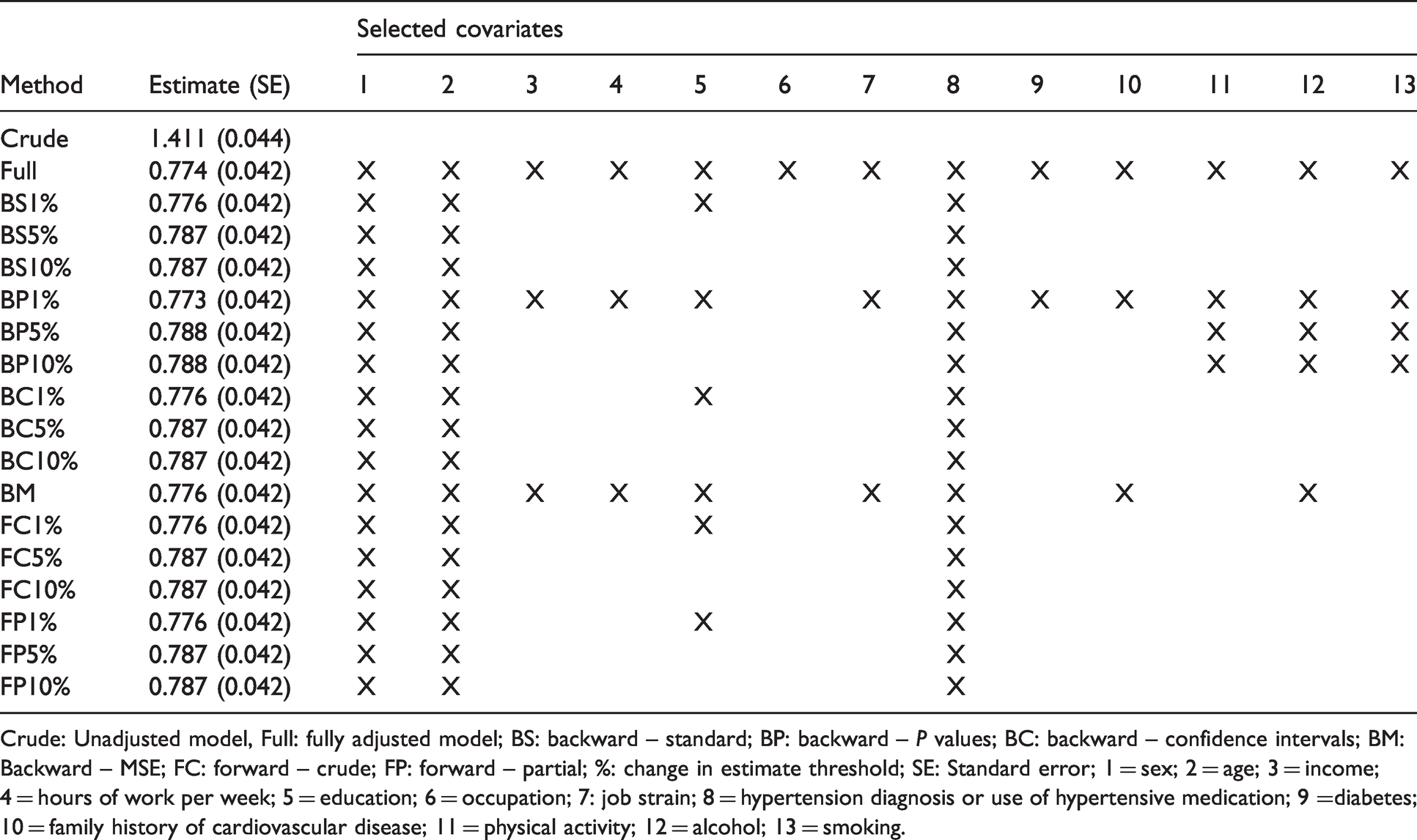
Crude: Unadjusted model, Full: fully adjusted model; BS: backward – standard; BP: backward – P values; BC: backward – confidence intervals; BM: Backward – MSE; FC: forward – crude; FP: forward – partial; %: change in estimate threshold; SE: Standard error; 1 = sex; 2 = age; 3 = income; 4 = hours of work per week; 5 = education; 6 = occupation; 7: job strain; 8 = hypertension diagnosis or use of hypertensive medication; 9 =diabetes; 10 = family history of cardiovascular disease; 11 = physical activity; 12 = alcohol; 13 = smoking.
Most methods had coverage rate below 90% in most scenarios. BC1% and BC5% had close to appropriate coverage in all scenarios with either
BS1%, BP1%, BC1% and BC5% had an RMSE similar to the one of the fully adjusted model in all scenarios. BS10%, FC5% and FC10% had mixed results, sometimes increasing, and sometimes decreasing the RMSE. BP10%, BM, FP5% and FP10% were the implementations that most consistently decreased the RMSE across scenarios. FP5% and FP10% were the most susceptible to yield an important decrease in the RMSE.
3.3 Time to event outcome
The results for the scenarios with a time to event outcome are displayed in Table 3 and Web Tables 11–15. In scenarios with
The coverage of 95% confidence intervals was below 90% in at least some scenarios for all methods. Only the fully adjusted model had close to appropriate coverage in all scenarios.
As in the binary outcome scenarios, BS1%, BP1%, BC1% and BC5% had an RMSE similar to the one of the fully adjusted model. BS10%, BP5%, BP10%, FC5% and FC10% increased the RMSE by more than 10% in one or more of the scenarios we considered. FP5% and FP10% were the methods that most consistently decreased the RMSE and that induced the greatest reduction in the RMSE.
3.4 Covariates inclusion
Table 4 presents the proportion of inclusion of covariates for each CIE implementation across simulation scenarios. The proportion of replicates in which a set sufficient to control confounding was effectively selected was less than 70% for all methods. This proportion was generally greater for smaller thresholds than for larger ones. On the other hand, most methods included instruments relatively often, sometimes as much as including all instruments in 100% of the replicates. This was particularly the case for smaller thresholds. Similarly, most methods also often included variables that are neither confounders nor instruments (“other” variables), especially with the 1% threshold. These results indicate that none of the implementation adequately differentiated confounders and non-confounders in our simulation study.
3.5 PROspective Québec (PROQ) study on work and health
To illustrate the change in estimate method in a real data setting, we explored the association between body mass index (BMI) and diastolic blood pressure (BP) in the PROspective Quebec (PROQ) Study on Work and Health. We note it would be possible (in fact, preferable) to instead draw a causal graph based on our subject-matter knowledge. However, since our goal is to illustrate and compare the different CIE implementations, we applied a naïve approach where all variables that were identified as potential confounders based on substantive knowledge are included in the variable selection procedures.
In Quebec City (QC, Canada) 9188 white-collar workers (48.5% women) enrolled in the PROQ cohort, were followed over a period of 25 years. 11 At recruitment, in 1991–1993, participants worked in one of 19 public and parapublic organizations in the Quebec City region. The eligibility criteria were to work at least 21 hours a week and not to hold another paid job of more than 10 h a week. The PROQ cohort had a participation rate of 75%. A first follow-up occurred in 1999–2001 with a participation rate of 89%. A second follow-up happened in 2015–2018, but is not considered in this analysis. This study was approved by the CHU de Québec – Université Laval’s ethical review board (#2012-1674).
BMI, a measure of body fat based on height and weight, has been positively associated with systolic and diastolic BP as well as with hypertension.17–20 The reduction of BMI combined with lifestyle modification are preferred strategies to reduce BP.21–23 Weight management strategies are supported by prospective evidence reporting that BMI reduction is associated with BP reduction, implying a causal relationship.18,24,25 Since BMI and BP are important cardiovascular risk factors, 26 this relationship has important implication, especially in population with high obesity rates.
We estimated the association between BMI at baseline and diastolic BP at the first follow-up using an unadjusted model, a fully adjusted linear regression, as well as the 16 CIE implementations considered in the previous section. Based on subject-matter knowledge, a set of 13 potential confounders measured at baseline was considered. This set included sex, age, income (in 1000 Canadian dollars), hours of work per week, education, occupation, exposure to job strain (a psychosocial work stressor), hypertension diagnosis or use of hypertension medication, self-reported diabetes, family history of cardiovascular disease, frequency of 20–30 minutes physical activity per month, number of alcohol drinks per week and current smoking (yes or no). Weight (kg) and height (cm) were measured by a trained research assistant. BMI was calculated by dividing a participant’s weight by their height in metres squared. BP was measured according to recognized protocol. 27 In brief, participant’s BP was measured at rest after they had been sitting for 5 min. The average of three BP measurements taken 1–2 minutes apart was recorded. More information is available elsewhere. 11 For the FP implementation, age and sex were forced to be included. To simplify the illustration, we considered a subsample of 6526 participants without missing data on any of the considered variables.
Table 5 provides descriptive statistics on these data. Among others, the proportion of female participants was lower among those with a BMI over the median (24.1 kg/m2) than those with a BMI below the median. Those with a greater BMI were also older, more likely to have a university diploma, suffered from hypertension or diabetes in a greater proportion, drank more alcohol and were less likely to be smokers. The linear association between BMI (in kg/m2) and diastolic BP (in mm Hg) estimated using the different methods is reported in Table 6. In this illustration, all methods produced similar point estimates, wherein each increase of 1 kg/m2 of BMI was associated with an increase of approximately 0.78 mm Hg of diastolic BP. Interestingly, all methods yielded virtually identical standard errors (0.042). Hence, in this example, employing the CIE to select potential confounders did not improve the apparent precision of the estimation. The covariates selected by the CIE implementations were also very similar. Age, sex and diagnosis of hypertension were always selected, and education was additionally included when a 1% threshold was used. Only the BP and BM implementations included further covariates.
4 Discussion
We have conducted an extensive simulation study that aimed at addressing a gap in knowledge regarding the performance of the CIE for selecting potential confounders. To the best of our knowledge, this is the first simulation study to consider scenarios with multiple potential confounders, with a continuous or a time to event outcome and to investigate the performance of forward inclusion and backward exclusion based on changes in confidence intervals implementations of the CIE.
In summary, we have observed that all CIE implementations are at risk of introducing substantial bias and to produce confidence intervals that include the true effect much less often than expected. Forward inclusion methods produced particularly poor results in terms of bias and coverage. Our results also indicate mixed performance of many CIE implementations in terms of reducing the RMSE. While most methods were able to achieve at least some reduction of the RMSE as compared to the fully adjusted models in some scenarios, the reduction was often modest and an increase in the RMSE could also occur. In such cases, the data-driven selection of confounders was harmful. In this regard, our results are similar to those of previous simulation studies.7–9 Forward CIE implementations were the most susceptible to substantially reduce the RMSE but were also the most likely to introduce important bias and yield invalid inferences. We have also observed that all CIE implementations failed to adequately differentiate confounders from non-confounders. The methods that were the most likely to include confounders were also the most likely to include instruments, which are particularly harmful for effect estimation. In the real data illustration, no reduction of the estimated standard error was observed, regardless of the implementation or threshold.
A limitation to consider when interpreting these results is that they arose from a synthetic data simulation study. Although a total of 54 different scenarios were considered, alternative scenarios may yield different results. Moreover, it is difficult to adequately replicate the complexity of real data using synthetic data simulations. Future studies may consider plasmode simulations, 28 which combine real and synthetic data, to address this issue. Another limitation concerns the non-collapsibility of the odds ratio and the hazard ratio. When non-collapsible effect measures are used, the change in estimate between different covariate adjustment sets may reflect non-collapsibility in addition to confounding. We attempted to mitigate this issue by estimating a true effect specific to the variables that were included in the final model. It would have also been possible to employ adjustment methods that circumvent the non-collapsibility issue by estimating marginal effects instead of conditional ones. When estimating a marginal effect, the effect measure is no longer conditional on the covariates that are included in the model, thus bypassing the non-collapsibility issue. Such methods notably include inverse probability weighting, standardization/g-formula, augmented inverse probability weighting and targeted maximum likelihood estimation.29,30 We did not consider these methods in the current study in an attempt to evaluate the CIE methods as they are currently being implemented in practice.
Despite these limitations, our results provide important insights concerning the CIE for selecting confounders. Considering the low ability of all CIE methods we have explored to yield unbiased estimates with improved precision and their inability to identify true confounders or valid inferences, there seems to be little or no benefit in employing any of the CIE implementation. An important point to consider is that CIE may give a false impression of improved precision when the estimated standard error is reduced after variable selection. However, this estimated standard error is invalid and underestimates the true standard error, since it does not account for the variability associated with the variable selection. Unfortunately, adequately accounting for the variable selection when estimating the standard error and producing confidence intervals is theoretically challenging.31,32 Although the usual bootstrap has been proposed, 14 this solution is not theoretically supported when the post-selection estimator is insufficiently smooth. 33
More sophisticated data-driven methods for confounder selection have been developed in recent years. Some of these methods address multiple of the shortcomings of the CIE that were observed in our study. For instance, they target an unbiased estimation of the casual effect with improved precision as compared to a fully adjusted model, and offer theoretical guarantees, under some assumptions, concerning the identification of true confounders in large sample sizes.12,34–40 However, causal thinking is always essential to adequately control confounding, notably to avoid adjusting for colliders or for variables lying on the causal pathway of interest (mediators) and to ensure that all known confounders are adjusted for.
Multiple tools and methods have been proposed to facilitate knowledge-based selection of covariates.5,13,41,42 Sensitivity analyses can also be used to explore the robustness of results to different choices of covariates when the role of some of them is unclear. As such, we believe that data-driven confounder selection should be considered as a potential complement to substantive knowledge only when it is unclear if some variables are true confounders or not; it should not be considered as a mandatory step of exposure effect estimation. Data-driven confounder selection methods may prove particularly helpful in new areas of research where expert knowledge is scarce, such as an emerging disease like COVID-19. When data-driven confounder selection seems warranted, we believe the CIE should be avoided since it offers little or no benefits and it can yield invalid estimates and inferences. Instead, the novel methods with a stronger theoretical background we mentioned earlier should be considered.
Supplemental Material
sj-pdf-1-smm-10.1177_09622802211034219 - Supplemental material for The change in estimate method for selecting confounders: A simulation study
Supplemental material, sj-pdf-1-smm-10.1177_09622802211034219 for The change in estimate method for selecting confounders: A simulation study by Denis Talbot, Awa Diop, Mathilde Lavigne-Robichaud and Chantal Brisson in Statistical Methods in Medical Research
Footnotes
Declaration of conflicting interests
The author(s) declared no potential conflicts of interest with respect to the research, authorship, and/or publication of this article.
Funding
The author(s) disclosed receipt of the following financial support for the research, authorship, and/or publication of this article: This work was supported by grants from the Fonds de recherche du Québec – Santé [#265385 to DT] and the Natural Sciences and Engineering Research Council of Canada [# 2016-06295 to DT]. DT is a Fonds de recherche du Québec – Santé Chercheur-Boursier (FRQS). MLR was supported by a FRQS training award for health professionals. The illustration’s data come from the PROspective Québec (PROQ) Study on Work and Health funded in large part by the Canadian Institutes of Health Research. Funding sources had no role in the design of the study, analysis and interpretation of the data, or in writing the manuscript.
Supplemental material
Supplemental material for this article is available online.
References
Supplementary Material
Please find the following supplemental material available below.
For Open Access articles published under a Creative Commons License, all supplemental material carries the same license as the article it is associated with.
For non-Open Access articles published, all supplemental material carries a non-exclusive license, and permission requests for re-use of supplemental material or any part of supplemental material shall be sent directly to the copyright owner as specified in the copyright notice associated with the article.