
Abstract
Cystic fibrosis is a chronic lung disease requiring frequent lung-function monitoring to track acute respiratory events (pulmonary exacerbations). The association between lung-function trajectory and time-to-first exacerbation can be characterized using joint longitudinal-survival modeling. Joint models specified through the shared parameter framework quantify the strength of association between such outcomes but do not incorporate latent sub-populations reflective of heterogeneous disease progression. Conversely, latent class joint models explicitly postulate the existence of sub-populations but do not directly quantify the strength of association. Furthermore, choosing the optimal number of classes using established metrics like deviance information criterion is computationally intensive in complex models. To overcome these limitations, we integrate latent classes in the shared parameter joint model through a fully Bayesian approach. To choose the optimal number of classes, we construct a mixture model assuming more latent classes than present in the data, thereby asymptotically “emptying” superfluous latent classes, provided the Dirichlet prior on class proportions is sufficiently uninformative. Model properties are evaluated in simulation studies. Application to data from the US Cystic Fibrosis Registry supports the existence of three sub-populations corresponding to lung-function trajectories with high initial forced expiratory volume in 1 s (FEV1), rapid FEV1 decline, and low but steady FEV1 progression. The association between FEV1 and hazard of exacerbation was negative in each class, but magnitude varied.
Keywords
Introduction
Cystic fibrosis (CF) is a lethal genetic disorder that primarily affects the lungs. The clinical course of CF is marked by progressive loss of lung function and typically results in respiratory failure. Forced expiratory volume in 1 s (hereafter, FEV1) is the most important clinical indicator in monitoring lung function decline in patients with CF. Patients during follow-up might experience acute respiratory events referred to as pulmonary exacerbations. It is, therefore, of clinical interest to characterize the association between the longitudinal outcome FEV1 and time-to-first exacerbation. The motivation for our research comes from the US CF Foundation Patient Registry that consists of patients that were monitored from 2003 until 2015. In particular, we examined a subset of the Registry, which consists of 1016 patients. These patients were six years and older and were observed with a median number of follow-up visits equal to six (with a range of 1–93 visits). The average age at baseline is 15 years (with a range of 6–21).
Several authors have studied the evolution of lung function over time, as summarized in a recent review; 1 however, to our knowledge, little work has been done regarding the association of the lung function such as FEV1 with time-to-event outcomes. In particular, joint modeling of longitudinal FEV1 and survival outcomes in CF was introduced several years ago, 2 but has not been further used in CF epidemiology due to the computational burden of this approach. Furthermore, it is well recognized that different unobserved sub-groups of the biomarker FEV1 exhibit different longitudinal profiles. 3 Patients can be categorized in several sub-groups (latent classes) with different trajectories. It is, therefore, of high clinical interest to measure the strength of association between FEV1 with the risk of first exacerbation accounting for the latent trajectories.
The joint model of longitudinal and survival data constitutes a popular framework to analyze longitudinal and survival outcomes simultaneously.4,5 In particular, two paradigms within this framework are the shared parameter joint models and the joint latent class models. The former paradigm links the longitudinal and the survival process via the random effects; however, it does not allow for latent classes.6–11 The latter paradigm, which associates the two processes through latent classes, explicitly postulates the existence of sub-populations.12–14 The main disadvantage of this approach is that there is no clear interpretation for the association of the two outcomes. In particular, it is not possible to obtain a parameter that quantifies the relationship between FEV1 and time-to-first exacerbation. The use of latent classes in the shared parameter model has been previously proposed in the framework of joint models of longitudinal and survival data. In particular, Jacqmin-Gadda et al. 15 focused on the evaluation of the conditional independence assumption by proposing a score test; however, the relationship between the longitudinal and survival outcome per class is not further discussed.
In our clinical application, we are mainly interested in quantifying the association between the longitudinal outcome FEV1 and the survival outcome time-to-first exacerbation using the shared parameter model. From the literature, it has been shown that sub-populations exist for the evolution of FEV1. 3 The aim of the paper is twofold. Firstly, to model the relationship between FEV1 and time-to-first exacerbation. For this purpose, we propose a Bayesian shared parameter joint model that integrates latent classes inherent in this heterogeneous population. This model will assess the strength of the association between the two outcomes while allowing for latent classes. Secondly, to address a problem that arises in latent class models, which is the selection of the optimal number of classes. Several approaches have been proposed in the literature both in frequentist and Bayesian frameworks, including among others the use of information criterion, Bayes factors, and reversible jump Markov chain Monte Carlo (MCMC). These approaches are computationally intensive and can require the fit of several models with different numbers of classes, which can be time-consuming. To overcome this problem, we will implement the method of Nasserinejad et al. 16 to our joint model. This method is a pragmatic extension of Rousseau and Mengersen 17 criterion that showed that when we overfit a mixture model by assuming more latent classes than present in the data, the superfluous latent classes will asymptotically become empty if the Dirichlet prior on the class proportions is sufficiently uninformative. Nasserinejad et al. 16 performed an extensive simulation study to further investigate this approach and used it as a criterion also in longitudinal studies for obtaining the optimal number of classes by simply excluding latent classes that are negligible in proportion.
Joint model estimation
Longitudinal submodel
To account for the fact that the population is heterogeneous and consists of G possible unobserved sub-groups, we postulate a latent class mixed-effects model.18–20 We let

According to the specification of the latent class mixed-effects submodel (1), both fixed and random effects are class-specific, whereas the measurement error
We let

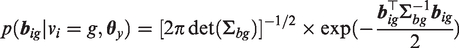
We employ a Bayesian approach where inference is based on the posterior distribution of the parameters in the model. We use MCMC methods to estimate the parameters of the proposed model. The likelihood of the model is derived under the assumption that the longitudinal and survival processes are independent given the random effects and the latent classes. Moreover, the longitudinal responses of each subject are assumed independent given the random effects and the latent classes. The likelihood contribution for the ith patient is written as

The likelihood contribution of the longitudinal outcome takes the form
The likelihood contribution of the survival model is given by
The posterior distribution is written as

A commonly used prior in mixture models for the class probability is a Dirichlet distribution. In particular
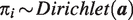
Small values of
Selection of number of classes
An important task in latent class models is to identify the optimal number of classes. Several approaches have been previously proposed for choosing the optimal number of classes in both frequentist and Bayesian settings. Common examples are the Bayesian information criterion (BIC), 21 deviance information criterion (DIC), 22 and other Bayesian approaches such as Bayes factor and reversible jump MCMC algorithm. 23 A drawback of the approaches above is that they are computationally intensive and some require the fit of models assuming different numbers of classes, which might be time-consuming for complex models such as the joint models of longitudinal and survival outcomes.
Furthermore, it has been previously discussed in the literature that a problem that arises in the calculation of the DIC in mixture models is that the posterior mean of the parameters may not lead to good predictive estimates. The MCMC parameters suffer from label switching, making the DIC (which is based on averaging over MCMC draws) unstable. A more appropriate choice for the estimates would be the mode of the posterior distribution. A wide range of options for constructing an appropriate DIC, including also mixture models, has been proposed by Celeux et al. 22 However, these are not straightforward to apply with existing software.
An interesting alternative was proposed by Rousseau and Mengersen,
17
where they proved that in overfitted mixture models (with more latent classes than present in the data), the superfluous latent classes will asymptomatically become empty if the Dirichlet prior on the class proportion is sufficiently uninformative. Recently, Nasserinejad et al.
16
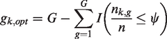
used this approach and proposed a latent class selection procedure for longitudinal models. An overfitted mixture model converged to the true mixture by assigning a small portion of individuals to empty classes, if the parameters of the Dirichlet prior First, a latent class model with a large enough number of latent classes is fitted. Then, the number of non-empty classes at each iteration is calculated as
After obtaining the non-empty classes per iteration, the posterior mode of the non-empty classes is calculated. Finally, the model with the optimal number of classes, which are the non-empty classes, is refitted.
where G is the total number of classes, k represents the iteration,
Advantages of this approach are that it is easy to implement even in such complex models, and it is not influenced by the label switching problem since we observe the non-empty classes at each iteration. The only time that we need to correct for label switching is when we fit the final model with the optimal number of classes. Furthermore, this approach requires us to fit the model only two times (namely one with the high number of classes and one with the optimal number of classes) instead of assuming all possible number of classes, therefore decreasing the computational burden. It has been shown through extensive simulations in the longitudinal setting that this method performs better than alternative model selection criteria such as BIC and DIC. 16
Simulations
We performed a series of simulations to validate the proposed model, to examine the class selection method on the joint modeling framework, and to explore the appropriate threshold that indicates a class as empty.
Design
We assumed around 1000 patients with maximum number of repeated measurements equal to 10. For simplicity, in this section, we ignore the notation for the latent classes (g). To simulate the continuous longitudinal outcome, we used the following linear mixed-effects model per data set. In particular


The baseline risk was simulated from a Weibull distribution
Under this setting, we simulated three different data sets that have different parameters for the fixed effects in the longitudinal submodel, the baseline covariates and baseline hazard in the survival submodel, the variance diagonal matrix of the random effects and the association parameter (more details are presented in Table 1). Figure 1 illustrates the evolution of the longitudinal outcome per gender from the simulation parameters for each one of the three data sets.
Simulation parameters for the three data sets.
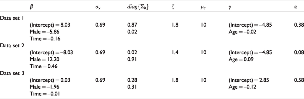
Simulation parameters for the three data sets.
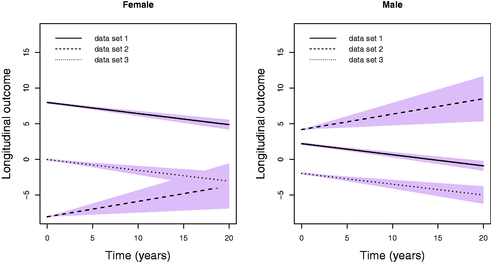
Evolution of the longitudinal outcome per gender from the simulation parameters for each one of the three data sets.
In order to investigate the proposed methodology, we assumed the three following scenarios. For Scenario I, we combined all three data sets assuming
diag{
where
We compared our proposed class selection methodology with the DIC criterion. Several adaptations have been proposed for mixture models by Celeux et al.
22
The parameters are not always identifiable, and the posterior mean of the parameters can be a poor estimator; therefore, in our simulation study, we assumed DIC3. A frequently used package, when the focus is on the association between a longitudinal and a survival outcome while taking into account that different sub-populations exist, is the
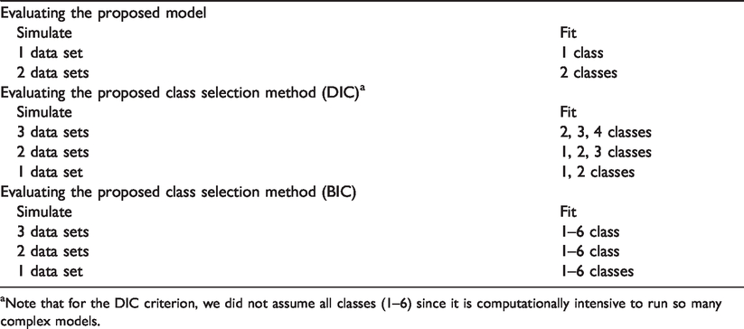
Simulation study overview.
Simulation study overview.
aNote that for the DIC criterion, we did not assume all classes (1–6) since it is computationally intensive to run so many complex models.
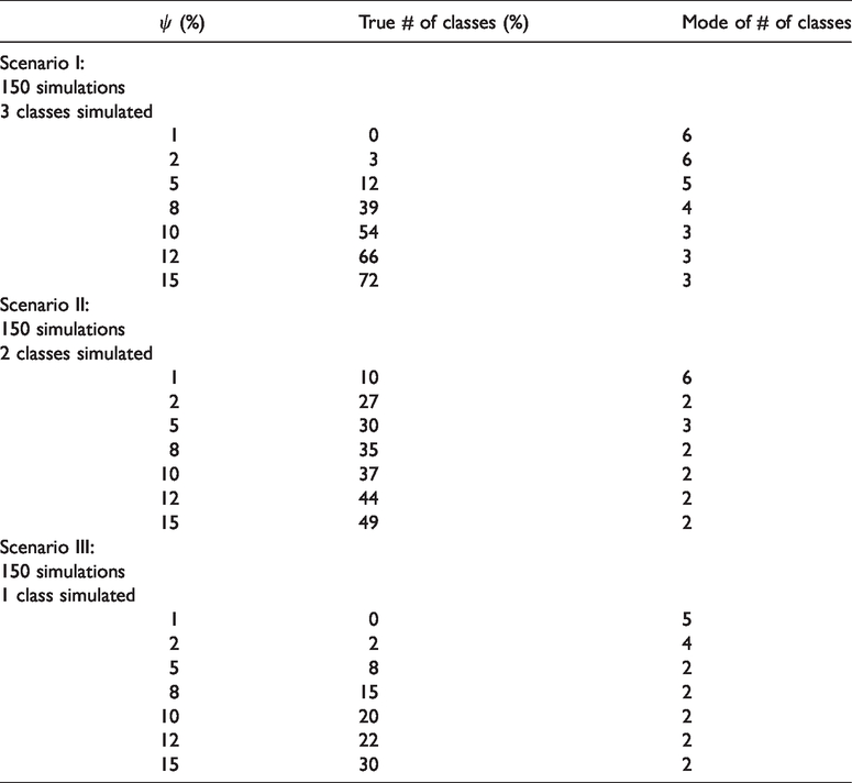
The results from the different scenarios for the validation of the proposed model are presented in Table 1 in the Supplementary Material. We obtain that the true parameters are close to the model parameters. The results from the different scenarios for the investigation of the proposed class selection approach are illustrated in Table 3. In particular, we present for different ψ the percentage of the true number of classes and the mode of the number of classes.
Simulation results: cut-off ψ, percentage of true number of classes, mode of the number of classes.
Simulation results: cut-off ψ, percentage of true number of classes, mode of the number of classes.
For Scenario I, we obtain the highest percentage when assuming ψ to be between 10 and 15%. In particular, assuming that the ψ is equal to 15% we obtain 72% of the time the correct number of classes and a mode equal to the correct number of classes (three). On the other hand, using the DIC and BIC criterion, we obtain 7% and 13% of the time the correct number of classes, respectively. Furthermore, both methods seem to underestimate the true number of classes (mode equal to one).
For Scenario II, we obtain the highest percentage when ψ is between 8 and 15%. In particular, assuming that the ψ is equal to 15% we obtain 49% of the time the correct number of classes and a mode equal to the correct number of classes (two). On the other hand, using the DIC and BIC criterion, we obtain 0% and 5% of the time the correct number of classes, respectively. Similar to Scenario I, both methods seem to underestimate the true number of classes (mode equal to one).
Finally, for Scenario III, the DIC and BIC criteria seem to perform better than the proposed approach, where it almost always selects the correct number of classes (one). This is not surprising since those criteria always underestimated the true number of classes in the previous scenarios. These results are also in line with previous work by Nasserinejad et al. 16 Using the proposed approach and assuming that the ψ is equal to 15%, we obtain 30% of the time, the correct number of class and a mode equal to two.
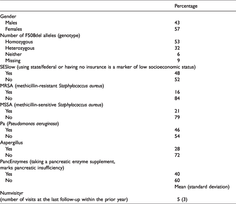
In this section, we present the analysis of the motivating data set. Our primary focus is to investigate the association between FEV1 and time-to-first exacerbation by taking into account that we have sub-groups with different evolution over time for FEV1. The first step is to obtain the optimal number of classes that can explain the heterogeneity of the population. From the literature, it is known that two or three classes are observed for the evolution of FEV1 outcome. 3 Therefore, for the selection process, we fitted a joint model assuming six classes. For the longitudinal outcome, we assumed a linear mixed-effects submodel including natural cubic splines for time (modeled as age, in years) with one internal knot at 15.84 years (corresponding to 50% of the observed follow-up times) in both the fixed and random effects parts. The DIC criterion and subject-specific plots (illustrating the observed and predicted values) were used to investigate the need for a non-linear evolution over time. Based on the DIC criterion, the best fit was obtained when using cubic splines with two knots. However, the observed versus predicted value plots did not show any drastic difference when assuming one knot; therefore, we decided to continue with the simplified model. Furthermore, we corrected for some baseline characteristics which were mainly based on clinical relevance and the literature. These variables, together with descriptive statistics, are presented in Table 4. In Figure 2, the FEV1 evolutions of 25 randomly selected patients with more than one repeated measurements are presented.
Descriptive statistics of the variables that were used in the model.
Descriptive statistics of the variables that were used in the model.
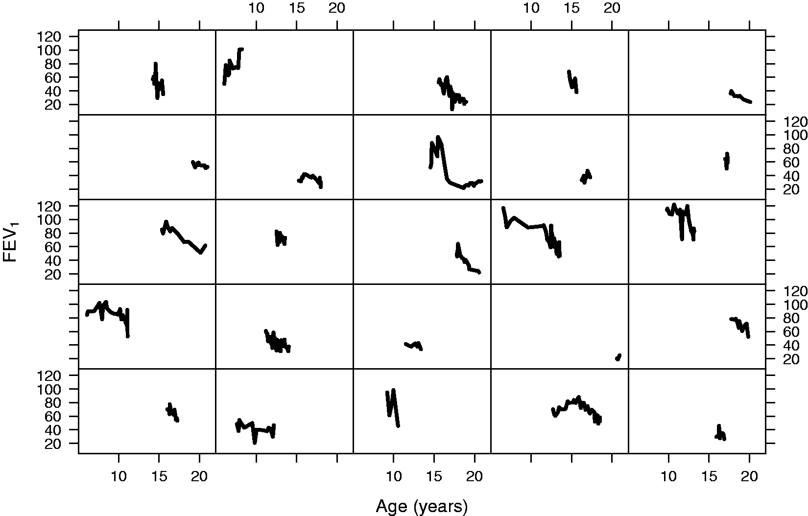
Individual FEV1 evolutions of 25 randomly selected patients with more than two repeated measurements.
Specifically, the model takes the form
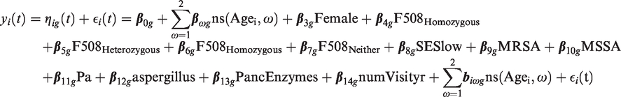
To investigate the association between FEV1 and time-to-first exacerbation, we postulated the proposed joint latent class model

For the baseline hazard, we assumed a quadratic B-splines basis with five internal knots placed at the corresponding percentiles of the observed event times ranging from 11.7 until 20.8 years.
In the Dirichlet distribution for the prior of the class probability, following the recommendation in Nasserinejad et al.,
16
we assumed
diag{
For the variance of the association parameter, no large value was required to ensure that we have a uninformative prior since with the standard joint model we obtained an association parameter smaller than 0.1. We ran the MCMC using a single chain with 500,000 iterations, 450,000 burn-in, and 100 thinning. The results indicate the presence of three or four classes, assuming that a class is empty if it contains 10 to 15% of the patients (10%
We reran the model assuming three classes and the normal scale of the continuous covariate age, numVisitsyr and FEV1 outcome. We ran the MCMC using 500,000 iterations, 450,000 burn-in, and 100 thinning. We, moreover, assumed two chains with different initial values to investigate the convergence towards local maximum. Density plots are presented in the Supplementary Material (Figures 1 to 5). We assumed the same priors as before except for
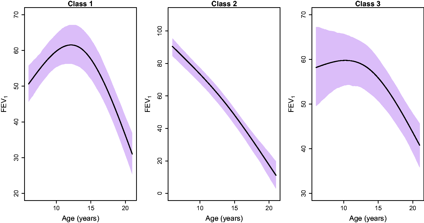
Evolution of the longitudinal outcome FEV1 per class assuming patients who are females, are F508del homozygotes, without low SES, are not infections with MRSA, MSSA, or Aspergillus, do not use pancreatic enzyme, do not have Pseudomonas aeruginosa and had five visits within the prior year which is the mean value of all observations. The plots illustrate the posterior mean and credible interval for each class.
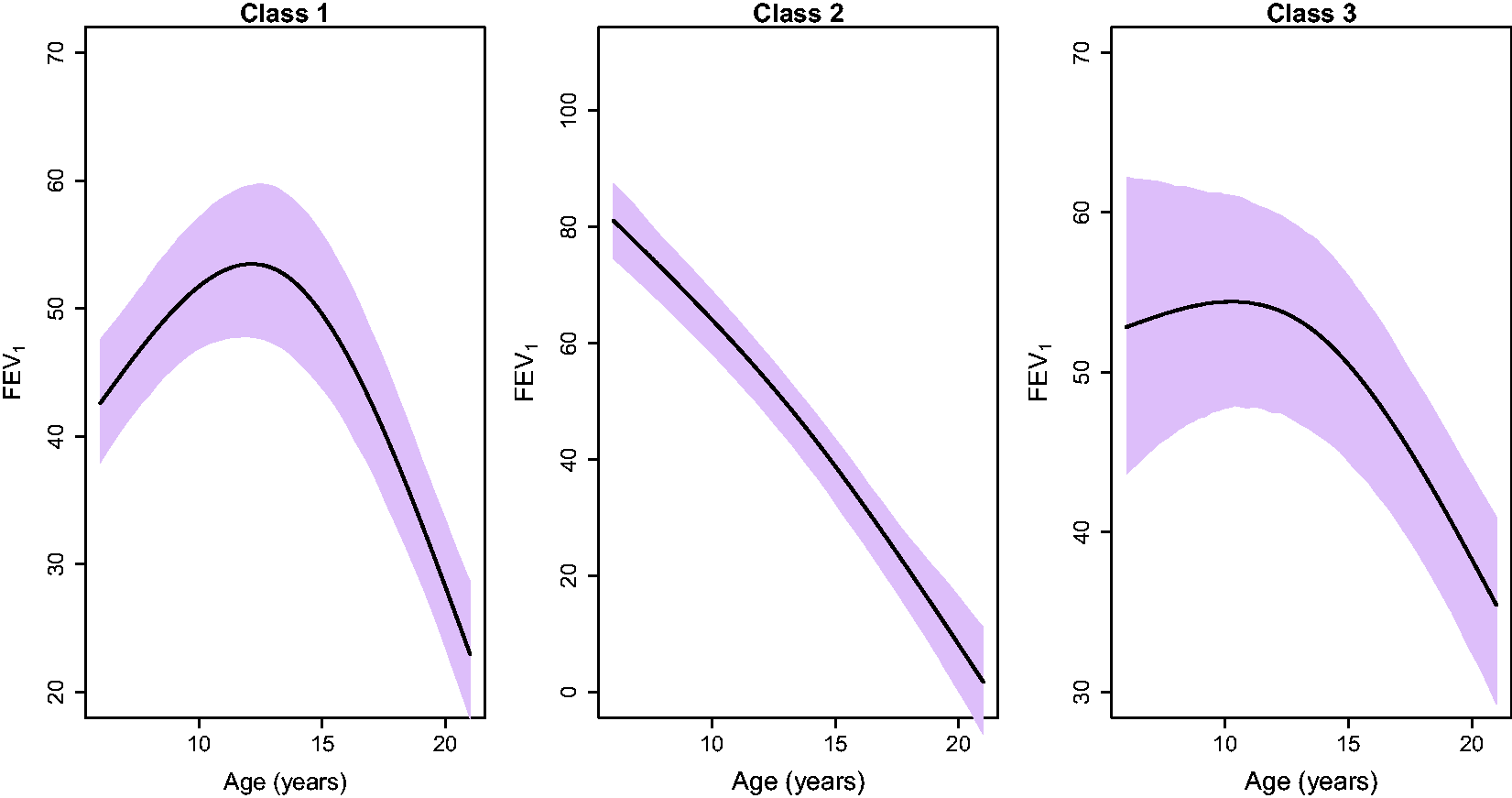
Evolution of the longitudinal outcome FEV1 per class assuming patients who are females, are F508del homozygotes, have low SES, are infections with MRSA, MSSA, Aspergillus, use pancreatic enzymes, have Pseudomonas aeruginosa and had eight visits within the prior year. The plots illustrate the posterior mean and credible interval for each class.
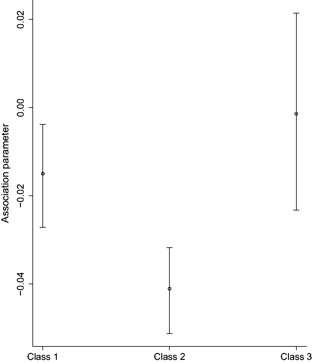
Mean and credible interval of the association parameter per class.
We, furthermore, examined this association parameter while ignoring the latent sub-populations. In that case, the association parameter is smaller than the largest parameter from our proposed model. This indicates that the use of a common association parameter for all sub-populations would lead to an underestimated/overestimated parameter for each group. Since it is expected that patients with a constant lung-function trajectory are less likely to experience exacerbation compared to the patients with a steeper decline, it is not realistic to assume a common association between the FEV1 evolution and time-to-first exacerbation for those group of patients.
In this paper, we proposed a shared parameter joint model incorporating latent classes. Applying it to CF data, this model accounted for patient heterogeneity inherent in the progression of FEV1. Compared to previously proposed joint latent class models, 13 we obtained the strength of the association between FEV1 and time-to-first exacerbation per group of patients. Finally, we focused on the selection of the optimal number of classes and used an overfitted mixture model (high number of classes) to obtain the non-empty classes.
A limitation of this approach is that it requires an intensive computational effort. In particular, for the class selection, where a model with a high number of classes is required, the number of parameters increases drastically. This, in combination with the high number of observations in the CF application increases the computational time that is required. Considering the difficulty of this model, it is almost impossible to obtain the optimal number of classes with other Bayesian criterion. Implementing the proposed criterion is straightforward; however, due to the complexity of the model, it is computationally expensive to fit a model with a larger number of classes, e.g. 10. It was shown in the simulation analysis that the DIC and BIC criteria always underestimated the true number of parameters, and it, therefore, performed better when the true number of classes was one. Even though in that scenario, the proposed method did not work perfectly, it seems to be better than other criteria and easier to perform.
The main limitation and challenge of the proposed approach is the choice of the threshold that indicates whether a class is empty or not. A simulation study was performed to investigate whether the proposed class selection method would be appropriate for the shared parameter models. An interesting finding was that the threshold was higher compared to simple approaches, such as mixed models. In particular, in our shared parameter model with integrated latent classes, the threshold was between 10% and 15%. In more simple settings, such as a linear mixed model that was extensively investigated with simulations by Nasserinejad et al., 16 this threshold was lower. Since this threshold highly depends on the complexity of the model, it is advisable to perform simulation studies to decide on a realistic cut-off when a different model is used. When no clear decision can be taken, our proposed criterion could be combined with other criteria to investigate the optimal number of classes in fewer models. Caution, however, is needed when using other criteria since we showed that the DIC and BIC performed worse in finding the correct number of classes. These results were in line with previous work by Nasserinejad et al. 16 The proposed approach led to the same number of classes as discussed in the CF literature on FEV1 trajectory classification; 3 , 25 therefore, we did not investigate further the number of classes using other criteria. A further limitation of the manuscript is that we did not investigate which functional form describes best the association between FEV1 and time-to-first exacerbation. In this work, we assumed the underlying values of FEV1 to be related to time-to-first exacerbation as a first step to establishing an association between the two outcomes;2,27,28 however, our future research focuses on investigating which functional form of FEV1 is associated with the survival outcome exacerbations. Furthermore, in our model, recurrent exacerbations and death are not taken into account. Although there is a large database available in the US Registry, we used only a subset in order to make it feasible to run the proposed model. This subset has particular characteristics, and it cannot be generalized to all patients in the Registry. Therefore, the presented results do not reflect the diversity of the whole database.
Possible extensions would be to include more covariates also in the survival submodel in order to take into account extra information regarding the patients. Furthermore, using the proposed model for obtaining future FEV1 measurement and time-to-first exacerbation probabilities could lead to more efficient treatment prioritization and clinical management for patients with CF. In this paper, we used an overfitted mixture model and a non-informative Dirichlet prior for the class proportion in order to obtain the optimal number of classes. Overviews of mixture modeling, mixtures of Dirichlet processes, and how to identify the optimal number of classes using a Dirichlet prior can be found in Escobar and West and in Frühwirth-Schnatter and Malsiner-Walli.29,30
Supplemental Material
sj-pdf-1-smm-10.1177_0962280220924680 - Supplemental material for Integrating latent classes in the Bayesian shared parameter joint model of longitudinal and survival outcomes
Supplemental material, sj-pdf-1-smm-10.1177_0962280220924680 for Integrating latent classes in the Bayesian shared parameter joint model of longitudinal and survival outcomes by Eleni-Rosalina Andrinopoulou, Kazem Nasserinejad, Rhonda Szczesniak and Dimitris Rizopoulos in Statistical Methods in Medical Research
Footnotes
Acknowledgements
The authors would like to thank the Cystic Fibrosis Foundation for the use of Cystic Fibrosis Foundation Patient Registry (CFFPR) data to conduct this study. Additionally, we would like to thank the patients, care providers, and clinic coordinators at Cystic Fibrosis centers throughout the United States for their contributions to the CFFPR. The authors would like to thank the two anonymous reviewers for critically reading the manuscript and suggesting substantial improvements.
Declaration of conflicting interests
The author(s) declared no potential conflicts of interest with respect to the research, authorship, and/or publication of this article.
Funding
The author(s) disclosed receipt of the following financial support for the research, authorship, and/or publication of this article: This study was funded by grants K25 HL125954 and R01 HL141286 from the National Heart, Lung and Blood Institute of the National Institutes of Health.
Supplemental material
Supplemental material for this article is available online.
References
Supplementary Material
Please find the following supplemental material available below.
For Open Access articles published under a Creative Commons License, all supplemental material carries the same license as the article it is associated with.
For non-Open Access articles published, all supplemental material carries a non-exclusive license, and permission requests for re-use of supplemental material or any part of supplemental material shall be sent directly to the copyright owner as specified in the copyright notice associated with the article.