
Abstract
The hazard function plays a central role in survival analysis. In a homogeneous population, the distribution of the time to event, described by the hazard, is the same for each individual. Heterogeneity in the distributions can be accounted for by including covariates in a model for the hazard, for instance a proportional hazards model. In this model, individuals with the same value of the covariates will have the same distribution. It is natural to think that not all covariates that are thought to influence the distribution of the survival outcome are included in the model. This implies that there is unobserved heterogeneity; individuals with the same value of the covariates may have different distributions. One way of accounting for this unobserved heterogeneity is to include random effects in the model. In the context of hazard models for time to event outcomes, such random effects are called frailties, and the resulting models are called frailty models. In this tutorial, we study frailty models for survival outcomes. We illustrate how frailties induce selection of healthier individuals among survivors, and show how shared frailties can be used to model positively dependent survival outcomes in clustered data. The Laplace transform of the frailty distribution plays a central role in relating the hazards, conditional on the frailty, to hazards and survival functions observed in a population. Available software, mainly in R, will be discussed, and the use of frailty models is illustrated in two different applications, one on center effects and the other on recurrent events.
Keywords
1 Introduction
The central concept in survival analysis is the hazard function. It describes the instantaneous risk of the event of interest for an individual, given that the individual has not experienced the event previously. The hazard function indirectly also describes the distribution of the time to event; there is a one-to-one relation between the probability of being alive over time, the survival function, and the hazard function. Individuals may differ with respect to their survival probabilities, or, equivalently, with respect to their hazards. Females tend to live longer than males, or in terms of hazards, the mortality rate of males is higher than that of females; patients with more severe disease tend to die earlier and have a higher hazard than less severely diseased patients. Such characteristics can be accounted for in survival models by including them in models for the hazards. The most influential of such models is Cox’s proportional hazards model. 1 The proportional hazards assumption specifies that the ratio of the hazards between any two individuals is constant over time, and the shape of the hazard is given by a non-parametric “baseline hazard”. If a model is perfectly specified, so that all possible relevant covariates are accounted for, then the baseline hazard reflects the randomness of the event time, given the value of covariates.
In practice, however, it is rarely possible to account for all relevant covariates. Then the explanatory variables account for observed heterogeneity, and the unaccounted part is termed unobserved heterogeneity. If this is the case, then the estimated hazard for a specific set of covariates does not have an individual interpretation. 2 Rather, it represents an average hazard function, where the average is taken at each time point over the individuals still alive at that time point. The effects of unobserved heterogeneity on life times are collectively referred to as frailty in demographic research. 3 The frailty is an unobserved individual random effect that acts multiplicatively on the hazard. The estimated spread of this random effect (e.g. variance) is an indication of the amount of unobserved heterogeneity. The frailty model quickly gained popularity in econometrics, 4 demographics 5 and biostatistics. 6
Frailty models are useful for two purposes. First, univariate frailty models can be used to explain effects of selection of healthier subjects over time, and also to explain lack of fit, such as deviations from the proportional hazards model. Frailty models can be used in this context to offer alternative explanations for the behavior of the hazard and of hazard ratios over time. These alternative explanations are hypothetical to a large degree, because of identifiability issues, but useful nonetheless. Second, in shared frailty models, frailties can also be used to model dependence of survival times in clustered data or recurrent events. Here the frailty term is shared among individuals in the same cluster, or, in the case of recurrent events, among subsequent events of the same individual.
The aim of this tutorial is to provide an overview of theory and practice in the field of frailty models, while offering insight into the problems that are addressed by such models. We concentrate on the use of frailty models in survival analysis. Frailties have also been used in, for instance, infectious disease modeling,7,8 but this is outside the scope of the present tutorial. For more detailed information, we recommend the books.9–11 In section 2 we study the effects of unobserved heterogeneity in survival data, univariate frailty models, and we discuss different frailty distributions. In section 3, we analyze the effect of unobserved heterogeneity in shared frailty models, covering clustered survival data, recurrent events, and an overview of estimation methods. In section 4, we compare available software packages for frailty models and the representation of event history data in the R statistical software. In section 5 we examine different extensions to the frailty models. Finally, in section 6, we illustrate the application of frailty models in two common situations, the modeling of center effects and the analysis of recurrent events.
2 Univariate frailty models
2.1 Heterogeneity in the Cox model
Before we introduce the frailty model and start discussing the effects of unobserved heterogeneity, we illustrate here some of these effects in the more familiar setting of the Cox proportional hazards model.
2.1.1 Heterogeneity over time
The Cox model specifies the hazard of a time to event T as

The risk set at time t is composed of individuals that have not yet experienced the event of interest and have not yet been removed for other reasons, such as censoring. The distribution of the covariates among the individuals in the risk set changes over time. We illustrate this by considering model (1) and a single covariate following a standard normal distribution
This is illustrated by simulating a single sample of life times of size n = 100, according to equation (1), with a covariate
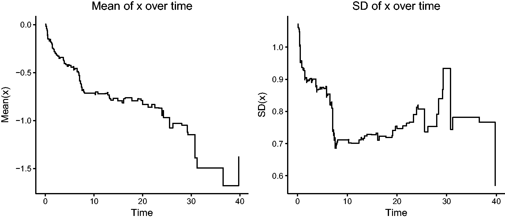
Changes in the mean and variance of a covariate x over time among survivors in a proportional hazards model.
2.1.2 Heterogeneity due to missing covariates
The proportional hazards assumption in the Cox model (1) specifies that the ratio

Assume that the model (1) is correct and
No evidence of violation of the proportional hazards assumption is found, when a test based on Schoenfeld residuals is used 13
However, when x2 is omitted, the resulting estimate of the effect of x1 is visibly smaller than 1:
Moreover, there is clear evidence against the proportional hazards assumption.
This is also illustrated by the plot of scaled Schoenfeld residuals of
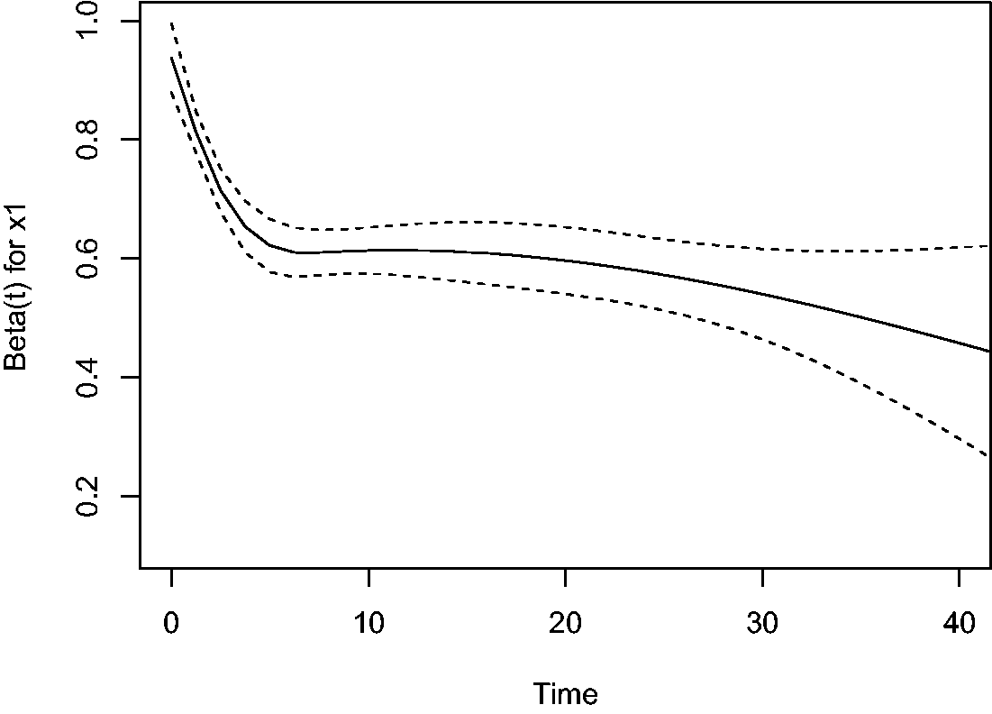
Plot of scaled Schoenfeld residuals-based
The explanation for the phenomenon illustrated in the simulated example is that the individual hazard is determined by the combined effect of x1 and x2. Since β1 and β2 are both positive, the “high risk” individuals (high x1, high x2) are the first to experience the event, on average, followed by the “moderate risk” ones (high x1 and low x2, or low x1 and high x2), and eventually the “low risk” ones (low x1 and low x2). This causes the correlation between x1 and x2, which is initially around 0, to become negative, as can be seen in Figure 3, where the sample correlation between x1 and x2 over time, among the survivors at the time, is shown in the large simulated data set. This phenomenon is also known in epidemiology as the obesity paradox. 17 The result of this negative correlation is that if x2 is not accounted for, the individuals with high x1 in the population of survivors artificially appear at lower risk than before, since they are likely to have a low value of x2, if they are still alive. This induced loss of independence has profound consequences. Suppose that x1 stands for a treatment in a randomized clinical trial. Since the treatment has been randomized, at randomization x1 may be expected to be independent of any measured or unmeasured characteristics influencing the time to the event of interest. Putting it differently, the distribution of these characteristics is expected to be the same for the randomized treatment arms at baseline. The above shows that this independence between x1 and the unmeasured characteristics can no longer be expected to hold at later points in time, ultimately implying that the hazard ratio is unsuited as a causal effect measure for survival data in the presence of unobserved heterogeneity.18,19
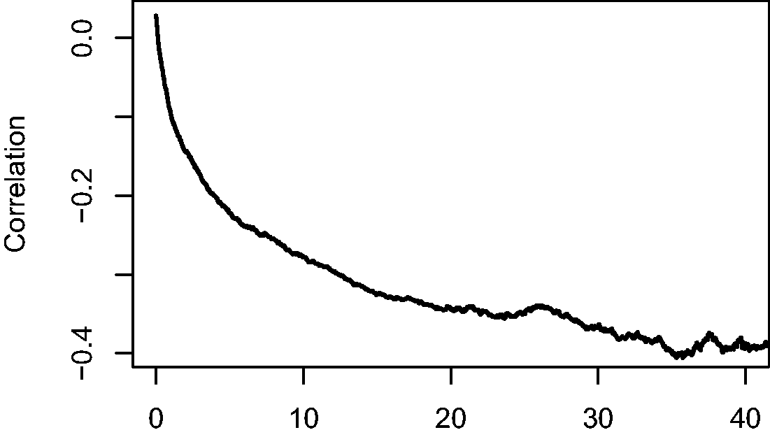
Correlation between x1 and x2 among survivors over time.
2.1.3 Conditional and marginal hazards
More generally, suppose that the proportional hazards model (1) holds for a covariate vector

Imagine that a Cox model is fitted only including
The
Since the effect of
2.2 The frailty model
A frailty model is a model for the hazards in which this unobserved heterogeneity is explicitly included as a multiplicative random effect, the frailty. In the univariate frailty model, the hazard of an individual with frailty Z is specified as

The frailty Z is a latent random term, assumed to have a certain non-negative distribution. Individuals with a higher frailty can be thought of as being more frail, and therefore expected to die sooner than other individuals with the same measured covariates. If the event of interest is a positive outcome, like pregnancy or recovery, subjects with a higher “frailty” are expected to experience the positive outcome sooner than others with the same covariates. For identifiability, Z is assumed to be scaled so that

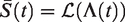
The survival function

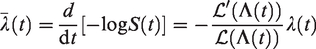
Unlike S(t),

A population averaged interpretation may also be given here:
The conditional and marginal hazards are equal only if
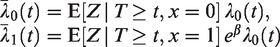
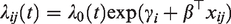
If observed covariates are also present, then it is usually assumed that the proportional hazards assumption holds conditional on the frailty, with

Then, the population averaged interpretations of
Regardless of whether the differences between individuals come from observed covariates
2.3 Frailty distributions
2.3.1 The Laplace transform
The Laplace transform turns out to be a very useful concept in describing relations between the conditional hazards and the marginal hazards and survival functions. The distribution of a non-negative random variable Z can be uniquely specified by its Laplace transform
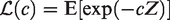
It is immediate that
Let us return to the frailty model of the previous section, where we wrote the hazard as
and the marginal hazard as
The Laplace transform of the frailty distribution of survivors can be easily expressed in terms of the Laplace transform of Z. First, denote the density of Z as f(z) and the density of
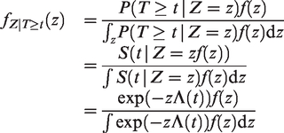
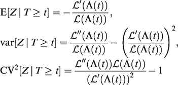
The Laplace transform of
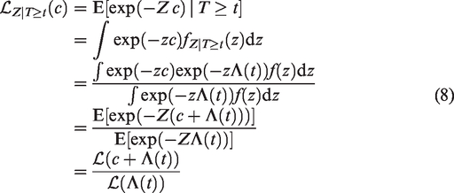
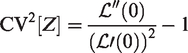
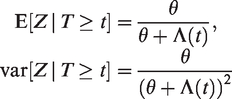
The expectation, variance and squared coefficient of variation of
2.3.2 Infinitely divisible distributions
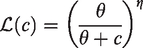
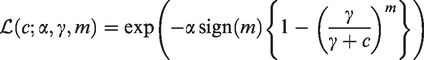
A rich family of frailty distributions with tractable Laplace transform are formed by the infinitely divisible distributions with Laplace transform specified as
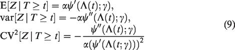
The unconditional expectation, variance and coefficient of variation of Z follow by replacing
The
Both functions reach their maximum over
A more general family of infinitely divisible distributions is the power-variance-function (PVF) family, with the Laplace transform The gamma frailty, obtained as a limiting case when The inverse Gaussian distribution, when The so-called Hougaard distributions, when m < 0; The compound Poisson distribution, when m > 0, which has probability mass The positive stable distribution, obtained as a limiting case when
2.3.3 Other frailty distributions
The
2.4 Frailty effects
The different frailty distributions discussed in section 2.3 represent different ways of expressing unobserved heterogeneity. Different frailty distributions lead to different selection effects, such as the one illustrated in section 2.1.1. Moreover, they impact the marginal effect of the observed covariates in different ways, generalizing the phenomenon illustrated in section 2.1.2. An advantage of the PVF family of distributions and their closed form Laplace transforms is that it facilitates the study of these phenomenons.5,6,26 An overview may be found in Aalen et al., 24 Chapter 6.
2.4.1 The selection effect
In section 2.3, it was shown that, for the gamma frailty model, the expectation and variance of the frailty distribution of the survivors decrease over time, in a similar way as illustrated in section 2.1.1. In Figure 4, we show the expectation and the variance of
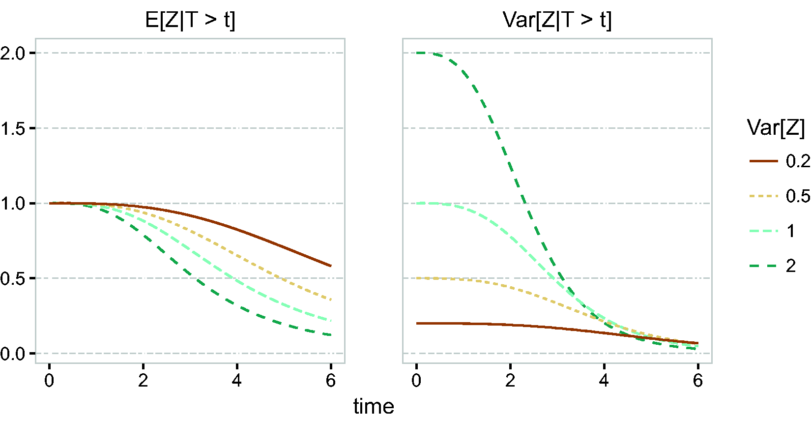
Frailty distribution of survivors, gamma frailty,
2.4.2 The marginal hazard ratio
In section 2.1.2, we illustrated that, when important covariates are omitted from a Cox model, the marginal effect of the remaining covariates is time-dependent. The same phenomenon happens with the marginal covariate effect in the case of frailty models. Suppose that only one observed covariate is present,
The marginal effect of x can be quantified by the ratio of these two marginal hazards. This results in
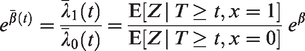
It follows that the original hazard ratio
If
Similar considerations apply for other frailty distributions. For example, for the inverse Gaussian distribution, the marginal hazard ratio is
In this case, we see that

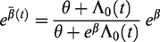
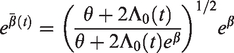
The effect of different frailty distributions on the hazard ratio is illustrated in Figure 5. For the gamma frailty distribution, the marginal hazard ratio approaches 1 with time, while for the inverse Gaussian it approaches
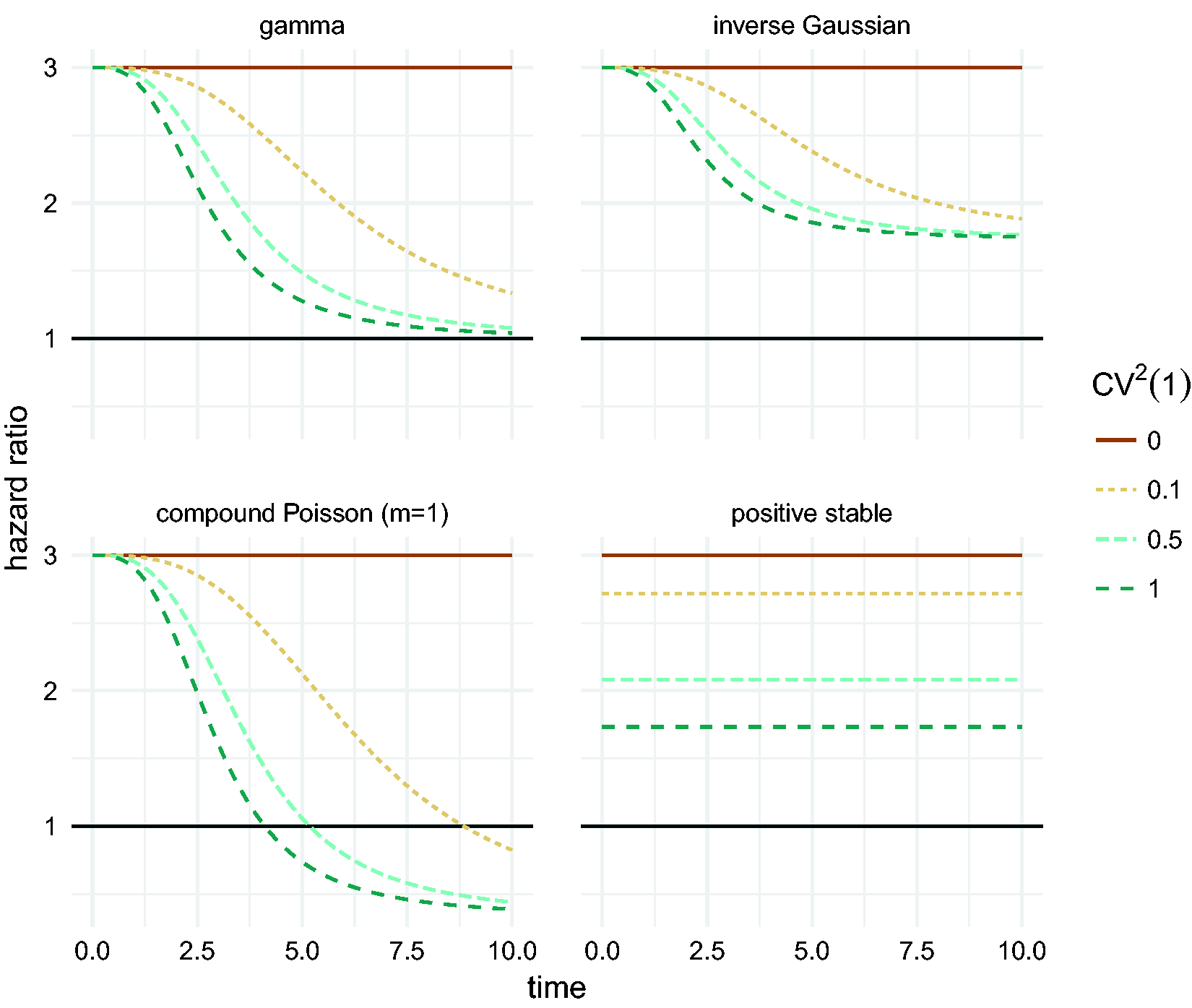
Marginal hazard ratio between two groups of individuals: a low risk one with
2.5 Identifiability
In the frailty model, the marginal hazard equals
Without further assumptions, observing a time-dependent covariate effect of the type shown in Figure 5 is equally compatible with (at least) two explanations. One is that the proportional hazards assumption holds in the conditional model, and this effect appears distorted at the marginal level as a result of unobserved heterogeneity. The second is that there is no unobserved heterogeneity, and the observed covariate has a time-dependent effect. In the first case, the frailty model is the natural choice. The frailty then explains heterogeneity due to unobserved covariates or other sources of natural variation. Even with an exhaustive set of covariates, the remaining natural between-subject variation can be explained by the frailty. In the second case, the modeling strategy would include a stratified analysis or an extended Cox model with interactions of covariates with time [Therneau and Grambsch, 12 Chapter 6.5]. Further explanations of violation of the proportional hazards assumption are discussed in Van Houwelingen and Putter, 28 Chapter 5.
In this context, the result of Elbers and Ridder, 27 while theoretically interesting, is of little practical use. Only a firm – and probably naïve – belief in the conditional proportional hazards assumption can substantiate a claim towards the presence of frailty. In principle, this situation changes in the case of clustered survival data, because positive correlation between the event times is induced by the frailty. This is discussed in section 3. The more information on the correlation structure, the easier it is to distinguish the presence of frailty from non-proportional hazards. However, when the cluster sizes are small, identifying the appropriate model remains a difficult problem because presence of frailty and violations of proportional hazards are confounded. 29
The positive stable distribution does not have finite expectation, and therefore it does not fall under the result of Elbers and Ridder. 27 As shown in Figure 5, it preserves the proportional hazards assumption at the marginal level. It is not identifiable with univariate survival data, even with covariates in a proportional hazards model. In some sense, this may be seen as an advantage, since it illustrates that the identifiability of univariate frailty models is based on a strong assumption about the mechanism that generated the data. The positive stable distribution does prove useful in the context of clustered failures or recurrent events in section 3.
Since the presence of frailty in a conditional proportional hazards model with univariate frailties is only identifiable through the distortion of the proportional hazards assumption in the marginal model, it follows that the frailty distribution is extremely hard to determine from such univariate data. Basically, it can be identified, assuming proportional hazards for the conditional model, only through the way in which the non-constant
3 Shared frailty models
In the previous section we used the familiar setting of the Cox model to illustrate some of the “odd effects of frailty”. 24 Also here, before introducing shared frailty models in clustered and recurrent events data, we will illustrate, again in the Cox model setting with shared covariates, some of the issues that turn out to play a role in shared frailty models.
3.1 Missing covariates in paired data
Consider the situation of paired event times, where covariate values are shared between individuals from the same pair. Assume that individuals from a given pair have the same distribution of the event time, denoted as T, with the hazard function
Consider one pair, with event times T1 and T2. The marginal survival function of either T1 or T2 is given by
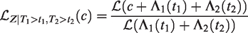
All this leads to a positive marginal correlation of the two life times. More specifically, it is straightforward to show that the marginal survival function of T2, given T1 = t1, is given by
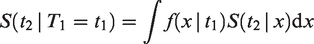
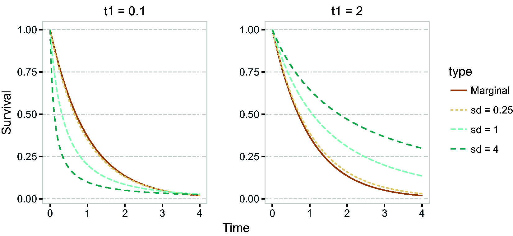
Conditional survival function of T2, given
It can be seen that for
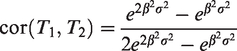
A plot of the correlation as a function of
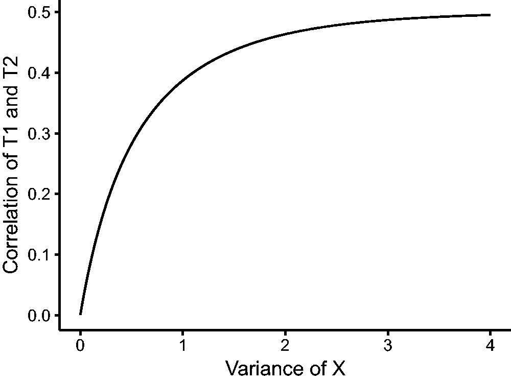
Correlation between T1 and T2 as a function of
If the correlation of life times cannot be explained by observed covariates (for example, because x is omitted), then there are two practical approaches. One is marginal modeling, which is in the spirit of general estimating equation (GEE) models. For the Cox model, this involves adjusting the standard errors of the observed covariates.
31
The second is to model the conditional hazard by introducing a “shared” frailty Z, that would take the place of
3.2 Clustered failures
3.2.1 The shared frailty model
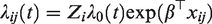
Assume that there are N clusters and ni individuals are part of cluster i. The hazard of the jth individual from cluster i is specified as

The individuals in cluster i share the frailty Zi, and conditional on Zi their lifetimes are assumed to be independent. While in the univariate case individuals are thought to be a random sample from a larger population of individuals, in the clustered failures case the clusters are thought to be an independent random sample from a population of clusters, and the individuals within a cluster are considered to be an independent random sample from a distribution specific to the cluster and further modified by covariates.
In the univariate case, the marginal survival function was derived, and also the marginal hazard. In the clustered failure case, we can derive the marginal joint survival function of a pair of individuals (or more), and it is useful to derive the posterior distribution of the frailty, given all information about the cluster, including observed events and censorings. This is studied in the next section.
3.2.2 Frailty distributions and clustered failures
Consider two individuals j = 1, 2 in the same cluster, with conditional hazards λ1 and λ2. The conditional cumulative hazards for these individuals are given by

The last equation follows from the assumed conditional independence of T1 and T2, given the frailty. The marginal joint survival probability is obtained by taking the expectation with respect to Z, which results in

There is a close connection with copulas, see for instance.
10
The Laplace transform of Z, given that individual 1 and 2 are alive at t1 and t2, is obtained, with the same arguments as in equation (8), as
The only difference from the univariate case is that
Assume now that the event time T1 of the first subject is observed at t1, and subject 2 is still seen to be alive at t2. Recall that the density of Tj is given by
The Laplace transform of Z, given

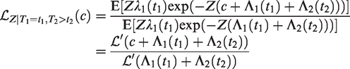
For a more detailed derivation, see equation (8). If both events are observed, the Laplace transform of Z given
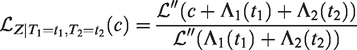
So far the Laplace transforms of the conditional distribution of Z, given T1 and T2, have been expressed in terms of generic hazard rates. Let us now turn to the situation where we have observed data from a cluster of arbitrary size, in which all subjects share the same frailty. Some of these observations include right-censored observations, for others the event of interest has been observed. Suppose we have a model that, conditional on observed covariates
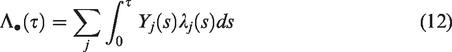
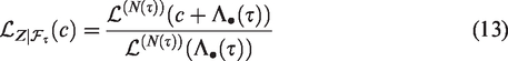
The expectation of this distribution follows as minus the derivative of its Laplace transform at c = 0
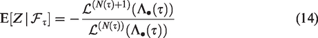
For the gamma frailty, we obtain that
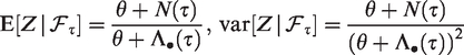
The class of infinitely divisible distributions, discussed in section 2.3.2, allows similar expressions to be derived.
3.2.3 Dependence and the cross-ratio
The estimated frailty variance offers an indication of unobserved heterogeneity between clusters, but it offers little information on the resulting marginal correlation of the event times. Even for paired data, the formulas for the bivariate survival function in equation (11) are difficult to interpret.
One measure of bivariate dependence is Kendall’s coefficient of concordance (Kendall’s tau). Denote two pairs of individuals as


This is proportional to the probability that the events within the same cluster are concordant, in the sense that they occur both before the median survival time or after. In frailty models, both τK and κ are positive quantities, since the specification (10) only allows for positive dependence. Under independence, both measures would be 0. However, the reverse statement is not usually true. Estimation of these coefficients in censored data is detailed in Hougaard, 9 Chapter 4.
A more natural way of exploring the within-cluster dependence structure is via the cross-ratio,
32
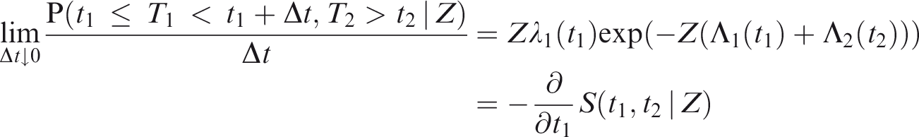
defined for pairs of subjects from the same cluster. It compares how the hazard of one subject in the pair would behave if an event would happen to the other subject, as opposed to an event not happening. Unlike τK and κ, it is a local measure of dependence. To illustrate this, we consider one cluster with individuals 1 and 2. Conditional on the frailty, their event times T1 and T2 are independent. Denote the hazard of individual 2 if individual 1 is alive at t1 as
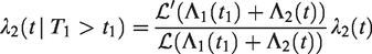
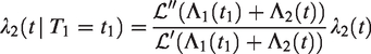
These two hazards concern different hypothetical event histories of the other individual in the cluster. They are equal only if there is no dependence between the two individuals. The cross-ratio can be expressed as
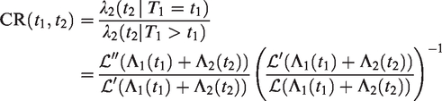
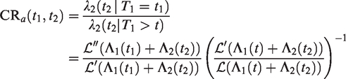
In Figure 8, we illustrate the unadjusted and adjusted cross-ratio functions for the gamma, inverse Gaussian and positive stable distributions. For comparison purposes, the distributions are matched by Kendall’s tau rather than variance. Both unadjusted and adjusted cross-ratio functions show that the hazard of individual 2 is larger if individual 1 has an event. The unadjusted cross-ratio for the gamma frailty is constant, showing that the event of individual 1 affects the hazard in the same way over time. The shape of the unadjusted cross-ratio for the inverse Gaussian and positive stable frailties shows that there is a strong immediate dependence that vanishes over time.
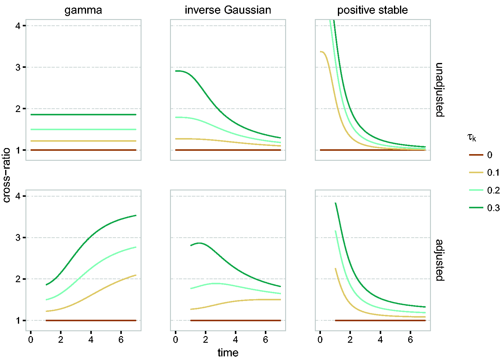
Cross-ratio (top row) and adjusted cross-ratio (bottom row, at
The adjusted cross-ratio paints a slightly different picture. For the gamma, it implies that, if one member of the pair dies, the hazard for the survivor would appear increasingly larger as compared to the scenario where the partner would still be alive. For the positive stable distribution, the surviving individual is at a perceived high risk right after the partner died, but the differences quickly decreases. This can be interpreted as a large correlation between the life times on the short term. As before, the inverse Gaussian is somewhere in the middle.
The unadjusted cross-ratio may be interpreted as an “instantaneous odds ratio”, 33 and for bivariate survival data it may be used for selecting the frailty distribution (Duchateau and Janssen, 10 Chapter 4). One disadvantage is that it depends on the conditional cumulative hazard; a scaled cross-ratio that overcomes this has been proposed by Paddy Farrington et al. 25
The gamma frailty is said to induce “late dependence” (a high probability of events occurring close by at later time points), the positive stable frailty induces “early dependence” (a high probability of event occurring close by early in the follow-up) and the inverse Gaussian is somewhere in the middle. The timing of the dependence can be studied by analyzing the joint distribution of T1 and T2. 9 A disadvantage of this approach is that the marginal distributions of T1 and T2 must be known separately, which is usually not possible.
3.2.4 Frailty model for recurrent events
Recurrent events are most commonly defined in the framework of counting processes. Each individual is described by a process N(t) that “counts” the number of events experienced by the individual until time t.
The two common frameworks for modeling N are the Poisson process and the renewal process.
34
If unobserved individual heterogeneity is present, then there are two approaches that may be used in practice. One is the marginal approach, where the unobserved heterogeneity is treated as a nuisance.
35
In that case, the focus of analysis is the marginal rate of N, which is defined as the probability of observing an increase in N in the small interval
The second approach is to model the intensity of N. While the hazard is defined as the instantaneous probability of an event given that the individual is alive, the intensity is defined as the instantaneous probability of an event given the whole previous event history of the individual. One way of incorporating the previous event history of the individual is to assume that the intensity at time t depends in some way on the number of events observed prior to time t. When the Poisson and renewal processes depend explicitly on the past, they result in so-called modulated Poisson and renewal processes. Another way is to implicitly model the dependence on the event history through a frailty Z. The conditional intensity of N, given Z, is then specified as

The marginal intensity is obtained by replacing Z by
The intensity in equation (15), with t referring to “time since origin of the recurrent event process”, is referred to as the calendar time or Andersen-Gill formulation. In the Andersen-Gill formulation, N is assumed to be a Poisson process, conditional on Z, meaning that its intensity conditional on Z does not depend on the history
In the case of recurrent events, the frailty mainly expresses that, if two individuals with identical covariates were observed over the same period of time, the expected number of events is larger for the one with the higher frailty. The number of events carries the most information on the frailty 9 (Chapter 9). Therefore, the measures of dependence discussed in subsection 3.2.3 are of little interest in this context.
Modeling recurrent events is a complex task and several types of models may be accommodated with counting processes (Therneau and Grambsch, 12 Section 8.5). Furthermore, time-dependent covariates representing, for example, the number of previous events, may also be added in the model (Aalen et al.,24 Chapter 8). A comprehensive reference on recurrent event modeling may be found in Cook and Lawless. 34
3.3 Estimation and inference for frailty models
Depending on the nature of the baseline hazard or intensity λ0, the frailty models may be classified as semi-parametric or parametric. In semi-parametric models, no assumptions are made on the baseline hazard or intensity λ0 and the maximum likelihood estimate of λ0 has mass only at the event times, as is the case for the Breslow estimator. 36 In parametric models, λ0 is determined by a small number of parameters, such as the exponential, Weibull or Gompertz models, or flexible parametric approaches employing spline-based estimators.
3.3.1 Likelihood and EM-based approaches
The likelihood construction for counting processes is detailed in most survival analysis textbooks.24,37 To cover all the scenarios described previously, assume that i denotes the cluster, (i, j) the j-th individual within the cluster i and tijk denotes the k-th event or censoring time observed on individual (i, j). We define the event indicator δijk as 1 if tijk is an event time and 0 otherwise. Suppose that the conditional hazard of subject (i, j), conditional on the frailty Zi is given by
Assuming that the frailties Zi are observed, the conditional likelihood contribution of cluster i is given by
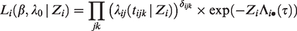
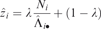
In the first part of this expression, Zi appears to the power Ni•, the total number of events from the cluster i. The marginal likelihood contribution of cluster i is obtained by taking the expectation over Zi

The parameters to be optimized are β, the vector of regression coefficients, λ0, the baseline hazard, and θ, the parameters of the frailty distribution, usually the frailty variance. For valid inference based on
For semi-parametric gamma frailty models, the Expectation-Maximization (EM) algorithm39 has been proposed.38,40 It can be extended in a straightforward way to the class of infinitely divisible distributions described in section 2.3.2.9,41 This involves iterating between two steps:
The “E” step, which involves calculating the expected log-likelihood
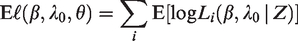
In practice, this involves calculating 2. The “M” step, where
The advantage of this approach is that the M step may be calculated via Cox’s partial likelihood,
42
effectively eliminating the problem of the high-dimensional λ0. For the E step, the “posterior” distribution of Zi, given the event history

This is available in closed form only for the gamma frailty, and is typically difficult to calculate for other frailty distributions. The expectation of this distribution,
3.3.2 Alternative approaches
The penalized likelihood method44,45 is a very popular way of estimating gamma and log-normal semi-parametric frailty models. The basic idea behind it is that, for fixed θ, the
Other approaches include a pseudo-likelihood method, 46 which leads to consistent estimators and may be employed for a larger number of frailty distributions, and the h-likelihood method.47,48 This approach relies on maximizing the joint likelihood of the observed and unobserved data. It has been developed for the gamma and log-normal distributions.
3.3.3 Inference
For parametric models, the variance–covariance matrix is typically obtained directly, as the inverse of the numeric Hessian matrix. This is usually provided directly by optimization software. For models estimated with the EM algorithm, Louis’ formula may be used 49 to obtain standard errors of the estimates. It has been shown that the baseline hazard may be regarded, for practical purposes, as an ordinary finite dimensional parameter and the information matrix may be constructed from the matrix of second derivatives. 50
For the profile EM algorithm, the variance covariance matrix for
Inference regarding the frailty variance is more challenging. The limiting case, when the variance is 0, is a proportional hazards model without frailty. A likelihood ratio test based on a 50:50 mixture of
4 Frailty models in practice
4.1 Software
Support for frailty models exists in major statistical packages such as R,
54
SAS
55
and Stata.
56
The
Semi-parametric gamma and log-normal frailty models may be estimated via the penalized likelihood method in the
Parametric and flexible parametric frailty models for the gamma and log-normal distributions are supported by the
4.2 Data representation
In R,
54
the canonical resources for survival analysis are found in the
An event history is represented by a collection of observations, which are vectors Recurrent events in calendar time (or “Andersen-Gill” representation). In this case, for an individual, tR are event times and tL is usually 0 or the time of the previous event. Usually, the last observation is censored with the last tR being the end of follow-up. Recurrent events in gap time. In this case, tL = 0 and tR are observed gap times. The last observation may be censored, indicating an incomplete gap time at the end of follow-up. Left truncated survival times, where tL is the time point after which the individual enters the study. Time-dependent covariates. In this case, if the value
In the presence of frailty, an observation is interpreted as a contribution to the conditional likelihood of the form

For a collection of observations sharing the same frailty Z, the software maximizes
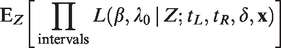
For left truncated survival times, however, this is generally incorrect. In the univariate case, the frailty distribution of a left truncated individual is that of
In the case of clustered survival times, the event of observing the whole cluster must be taken into account.66–68 If the individuals from the same cluster have truncation times
More complicated selection schemes arise when the left truncation times are not independent, even conditional on the frailty. 69 In the case of recurrent events, such selection schemes may arise when individuals are included into the study only if they experience a certain number of events. 70 Such scenarios usually require ad-hoc estimation procedures and are not generally supported by the main software packages.
In R, one of the reasons why the same notation is used to denote both recurrent events and left truncation is because they lead to the same likelihood in frailty-less models. In the case of frailty models, the treatment depends on the package used. For example, the
5 Extensions
The standard shared frailty model assumes that the frailty is shared among all individuals in the same cluster. This assumption can be relaxed by assuming that the frailty terms of individuals in the same cluster are not shared, but correlated.7,11,71,72 Correlated frailty models address the limitation that shared frailty models may only be employed for positively correlated event times.
Furthermore, so far the random effect Z has been assumed to be time-constant. This is consistent with the interpretation that Z accounts for individual specific or cluster specific characteristics that are fixed from the time origin, and have an effect that is constant over time. However, the unobserved heterogeneity might be time-dependent, thus better explained by an unobserved random process that unfolds over time. Several approaches based on this idea have been proposed. The frailty may be modeled with diffusion processes73,74 or Levy processes.
75
More recently, an approach on birth-death Poisson processes has been proposed.
51
Simpler, piecewise constant, frailty models have also been considered.76,77 A limited implementation combining the birth-death processes and the piecewise constant frailty is implemented in the R package
Since the models presented in sections 2 and 3 are intended for the analysis of one stochastic event process, it has been assumed that the censoring does not depend on the frailty included in the time to event model. This assumption may be tested, 82 and in case a violation of this independence assumption is detected, the event and censoring processes can be modeled jointly. An example is when the observation recurrent event process may be stopped by death 83 or when the frailty is also associated with the censoring. 84
Moreover, we assumed that in case of time-dependent covariates, the vector
More advanced random effect structures may be, in theory, considered. For example, if individuals experience recurrent events and are nested within clusters, a hierarchical random effects model may be considered. This is, however, not easily done in practice, and there is no standard software that currently supports such models.
6 Illustration
We end by discussing two illustrations of the use of frailty models. The first is a study on center effects in a breast cancer study, the second on recurrent events in patients with chronic granulomatous disease. The R code for the analyses performed is available as Supplementary Material.
6.1 Frailty models for center comparisons
The data originate from a clinical trial in breast cancer patients, conducted by the European Organization for Research and Treatment of Cancer (EORTC-trial 10854). The objective of the trial was to study whether a short intensive course of perioperative chemotherapy yields better therapeutic results than surgery alone. The trial included patients with early breast cancer, who underwent either radical mastectomy or breast conserving therapy before being randomized. The trial consisted of 2795 patients, randomized to either perioperative chemotherapy or no perioperative chemotherapy. Results of the trial were reported in literature.87,88 The data have been studied in a multi-state model in Putter et al. 89 and Van Houwelingen and Putter. 28 This data is based on a subset of all 2687 patients with complete information on all covariates used below. For descriptives on these covariates, see Van Houwelingen and Putter, 28 Appendix A.2.
In the trial, patients have been included in 15 participating centers. The size of the centers varies between 6 patients (the smallest one) and 880 (the largest), as illustrated in Figure 9.
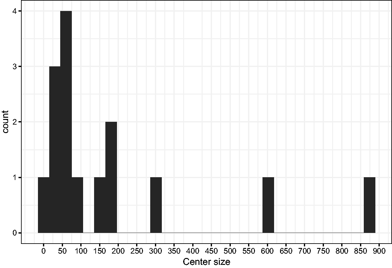
Histogram of center sizes.
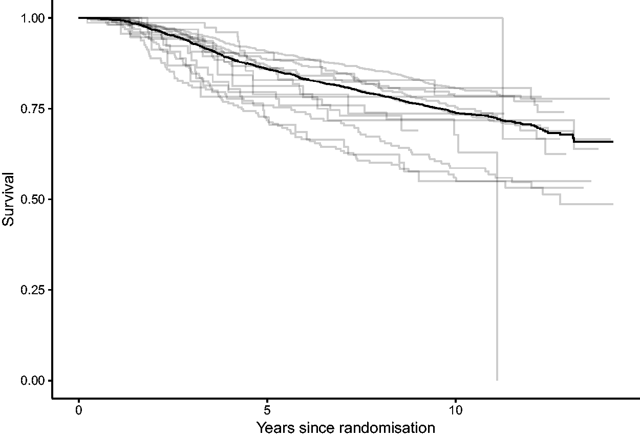
Kaplan–Meier survival estimates, overall and by center.
For this illustration, the endpoint of interest is overall survival. In Figure 10, we show the Kaplan–Meier estimates corresponding to each center (gray) and the overall estimate (black). These survival curves do not make it easy to compare centers. One of the reasons is that the survival curves are not controlled for possible differences between the distribution of covariates across centers (so-called case-mix), another is that it is difficult to disentangle randomness from systematic differences between centers.
For the inclusion of covariates, we start with a proportional hazards model, where the hazard of subject j from center i, given its covariates
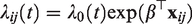
This model does not yet include any differences between centers. Estimating it is straightforward in principle, but for the standard maximum likelihood approach, the event times of the individuals are assumed to be independent. This assumption might not hold when observations come from the same center. Generalized estimating equations (GEE), with independent working covariance, may be used to obtain valid (sandwich) standard errors in this case. The results, with unadjusted and adjusted (robust) standard errors, are shown in Table 1, under “Cox model”. The hazard ratios
Estimates from the Cox model, the fixed effects model, the gamma and log-normal frailty models.
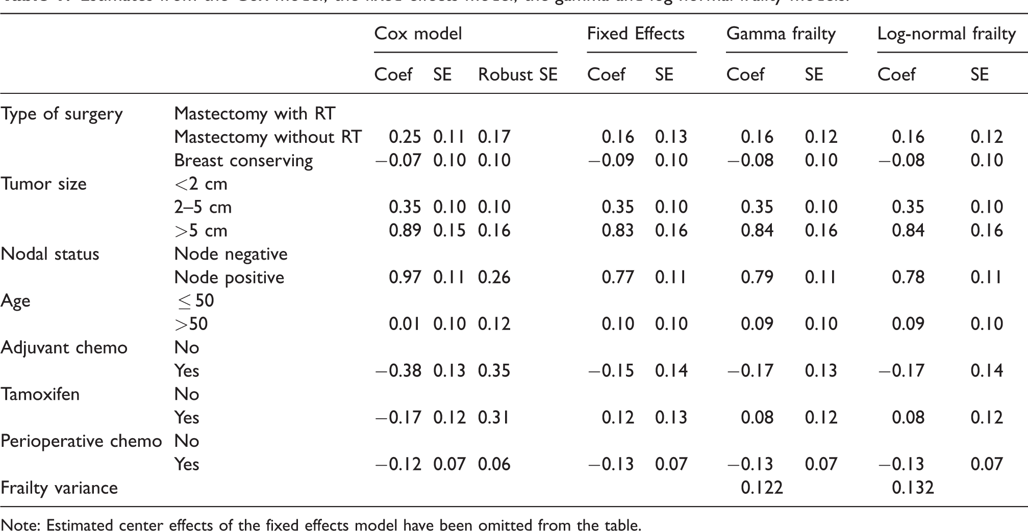
Note: Estimated center effects of the fixed effects model have been omitted from the table.
To explain more of the underlying heterogeneity, we account for center effects. The centers are included in a fixed effects model. The underlying model would be given by
Such a model can be fitted using center as a factor variable, taking one of the centers, usually the first, as reference center. The resulting estimates of the regression coefficients are shown in Table 1, under Fixed Effects. We can visually assess the differences between centers via a caterpillar plot, shown in Figure 11. The error bars denoted with “fixed effects” correspond to the estimates and 95% confidence intervals of the fixed effects estimates. In the Cox model estimated above, the first center is taken as reference, with an implicit
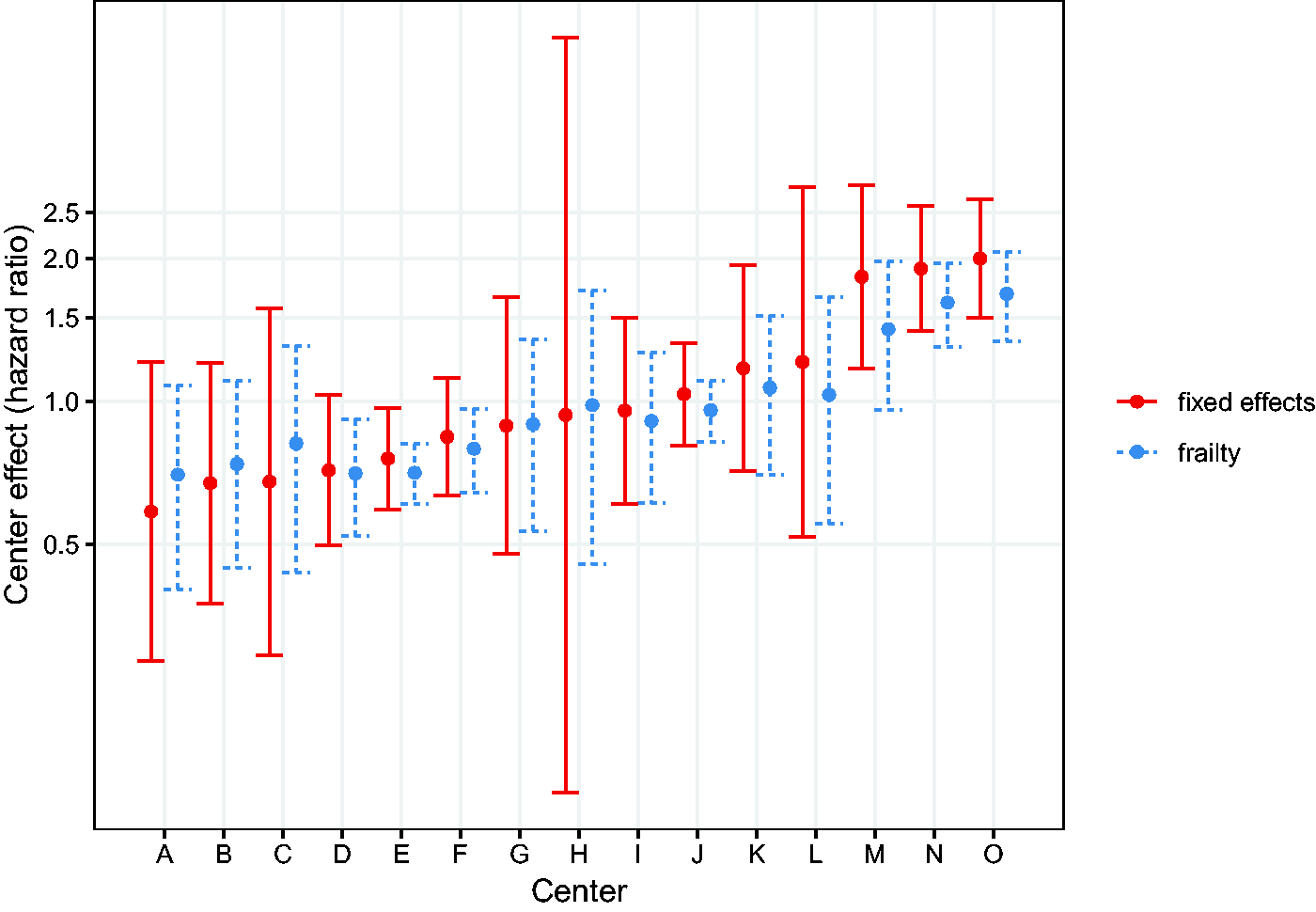
Center effects from the fixed effects and frailty models, expressed in hazard ratios.
More naturally, we would think about the centers as being randomly drawn from a population of centers, and their effects as being realizations from a frailty distribution. The underlying model would be
It may be observed that, particularly for the extreme centers, the frailty estimates are shrunken towards the mean (1). In terms of interpretation of the frailty estimates, it is helpful to study the form of the empirical Bayes estimates. For the gamma frailty model, it may be shown that the empirical Bayes estimate for center i is given by
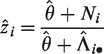
with

Therefore,
The proportional hazards assumption may be checked with, for example, with a test based on residuals. 13 In the case of the Cox model, this tests shows evidence against non-proportionality for tumor size and nodal status. For the frailty model, the same test can be carried out on the same Cox model, but with the logarithm of the log-frailties as offset. In this case, the conclusions are unchanged and indicate that further modeling of these variables may be required. Note that this may not be the case if the clusters would be smaller in size; we discuss this in section 7.
For comparison, we also estimated the same model with log-normal instead of gamma frailty. The maximized likelihood of this model was −5449.4 versus −5450.9 for the gamma frailty, suggesting a better fit to the data. The estimates of the regression coefficients are also shown in Table 1. The results from the two models are virtually identical, except for the estimated frailty variance which is slightly larger than the one from the gamma frailty.
6.2 Frailty models for recurrent events
The data are from a placebo controlled trial of gamma interferon in chronic granulomatous disease (CGD) and are available in the
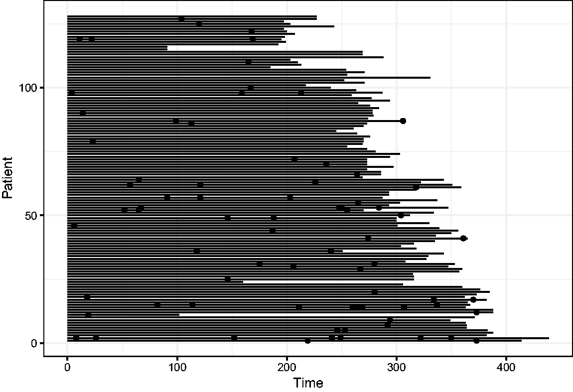
Event history of the CGD data. The length of the line indicates the length of follow-up, and the dots indicate the infections.
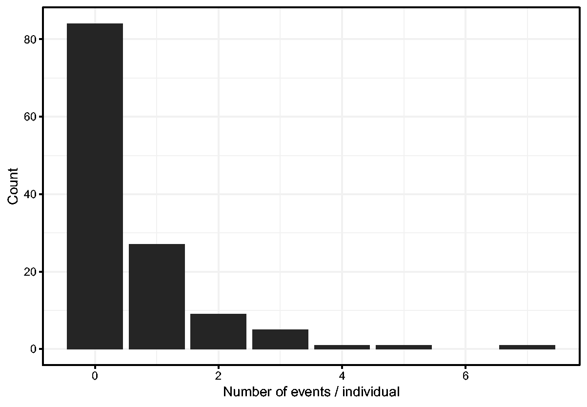
Histogram of number of events per individual.
A preliminary Cox model fit reveals that the treatment is highly significant, and that age, inherit and steroid usage are also significant. For the purpose of illustration, we will include these variables, plus sex, from now on. The results from the Cox model with these selected covariates are shown in Table 2. The covariates explain part of the differences between intensities in the occurrence of infections between the individuals. To quantify the unobserved heterogeneity in the intensities, we fit a shared gamma frailty model to the data. The frailties reflect the increase or decrease in infection rates of different individuals. The result is shown in Table 2. The frailty variance is estimated as 0.555, with (profile) likelihood ratio test-based 95% confidence interval
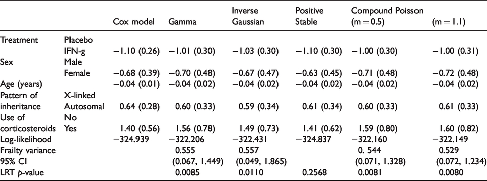
Estimates of the regression coefficients and fit summary from the Cox model and shared frailty models, with gamma, inverse Gaussian, positive stable and compound Poisson (with parameters 0.5 and 1.1) distributions, fitted on the CGD data.
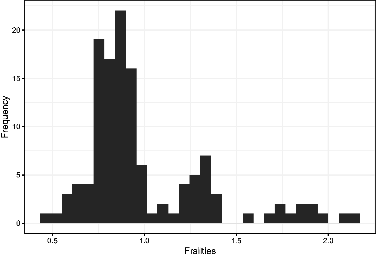
Histogram of the estimated frailties.
It is possible to question our choice for the gamma frailty. Partially due to software limitations, other distributions are rarely considered in practice. Table 2 also shows estimated frailty variances with 95% confidence intervals, as well as marginal log-likelihoods of fitted frailty models with other frailty distributions, including the inverse Gaussian, compound Poisson (m = 0.5), and positive stable distributions. Recall that the inverse Gaussian is a particular case of the PVF distributions. So is the compound Poisson distribution, where the parameter m, initially chosen as 0.5, determines the actual distribution. A grid search among possible values of the m parameter of the compound Poisson distribution (from 0.2 to 2.0 in steps of 0.1) identified m = 1.1 as optimal value, in terms of maximizing the log-likelihood. The small differences between the log-likelihoods for different values of m, however, indicate that no clear difference can be seen between any of the compound Poisson distributions. It is notoriously difficult to choose between frailty distributions; in practice this choice is usually made by convenience.
The positive stable distribution is interesting to note. As mentioned before it does not have finite mean or variance; in contrast to the other frailty models, the fit of the positive stable frailty model is not deemed significantly better than that of the Cox model without frailty, by the likelihood ratio test.
In a sense, a frailty model implies that the marginal intensity of the counting process, given the past, depends on the previous number of events, through
7 Practical modeling advice
In practice, one would fit the frailty model for clustered survival data or recurrent event modeling. For univariate survival data, estimating frailty models involves a large degree of speculation, and their practical value is therefore limited. Nevertheless, they are useful tools in situations where there is a strong a priori evidence for heterogeneity, as for example in modeling time to pregnancy, 90 or when the objective is to understand or provide alternative explanations of the shape of the hazard. 91
In the context of clustered survival data, one would fit a frailty model for estimating covariate effects while adjusting for, and with the objective of quantifying the between-cluster heterogeneity. In the context of recurrent event data, one would fit a frailty model for estimating covariate effects without assuming that the recurrent event process is Poisson and quantifying the between-subject heterogeneity. The usage of random effects is particularly sensible when the clusters (or individuals, in the case of recurrent events) are considered to be a random sample from a larger population.
The starting point for modeling is typically a marginal model, using the GEE approach. The point estimates for covariate effects are obtained from a proportional hazards model, and the standard errors are calculated using a sandwich estimator. With coxph, for example, this may be obtained with the +cluster() option. In some cases, this explanation may suffice. The hazard ratios in such a marginal model quantify the effect of the covariates at the population level.
When the clusters are large in size, or when individuals have numerous recurrent events, one may consider including cluster-specific (or individual-specific, in the case of recurrent events) fixed effects. The variability of these fixed effects may be assessed informally, as illustrated in section 6.1. A meaningful variability would indicate the presence of unobserved heterogeneity. One issue with this is that the fixed effects estimates of the clusters with few subjects will have a large variability, and shrinkage towards the mean would be desirable. This was also illustrated in the same section. All frailty distributions will provide some degree of shrinkage, but only for the gamma and a limited set of other frailty distributions closed-form results are easily available. One way to formally evaluate the presence of unobserved heterogeneity is with the Commenges-Andersen score test. In practice, a frailty model may be useful to be estimated anyway, to be able to quantify the heterogeneity and formally evaluate the improvement in model fit via the likelihood ratio test.
In terms of choosing which frailty distribution is most appropriate, we start with the practical considerations. The gamma frailty model is the simplest and most well understood frailty model, and may be estimated by the base R survival package. Furthermore, theoretical results indicate that the gamma distribution is the limiting distribution of the frailty of long-time survivors,
92
irrespective of the frailty distribution at baseline. The log-normal frailty model is conceptually simple as well, since it involves considering an additive random effect on the same scale as the other covariates. This can also be estimated by the
In principle, different frailty models may be compared via their log-likelihoods. Such a procedure might be useful for selecting a well-fitting frailty distribution from a larger class of frailty distributions, such as the power variance family, but since the frailties are latent, there typically is not a lot of information in the data to make a well informed choice, as could also be seen in section 6.2. Since the gamma frailty distribution is the most popular frailty distribution, a number of procedures for testing goodness-of-fit of the frailty distribution in the shared gamma frailty model have been proposed. Shih and Louis 93 suggest to visually assess the fit of the gamma frailty distribution by plotting the empirical Bayes estimators of the frailties given the observable data so far over time. For the gamma frailty model, these should be constant over time. This test was later extended by Glidden. 94 Geerdens et al. 95 developed a goodness-of-fit test by constructing a class of frailty model that extend the gamma frailty model using polynomial expansions that are orthogonal to the gamma density. The aforementioned tests focus on the goodness-of-fit of the gamma frailty distribution in the gamma frailty model. When evaluating the fit of a proportional hazards frailty model, another aspect is the validity of the (conditional) proportional hazards assumption. This assumption may be assessed in a similar way as in a regular survival model, by including the logarithm of the empirical Bayes frailty estimates as an offset in the proportional hazards model, and studying the Schoenfeld residuals. 12 This is most sensible when cluster sizes are relatively large (e.g. above 10 subjects). When this is not the case, the presence of frailty and the proportional hazards assumption may still be, to some extent, confounded. 29
Supplemental Material
sj-zip-1-smm-10.1177_0962280220921889 - Supplemental material for A tutorial on frailty models
Supplemental material, sj-zip-1-smm-10.1177_0962280220921889 for A tutorial on frailty models by Theodor A Balan and Hein Putter in Statistical Methods in Medical Research
Footnotes
Acknowledgement
The European Organisation for Research and Treatment of Cancer (EORTC) is gratefully acknowledged for making available anonimized data of the EORTC-10854 trial.
Declaration of conflicting interests
The author(s) declared no potential conflicts of interest with respect to the research, authorship, and/or publication of this article.
Funding
The author(s) received no financial support for the research, authorship, and/or publication of this article.
References
Supplementary Material
Please find the following supplemental material available below.
For Open Access articles published under a Creative Commons License, all supplemental material carries the same license as the article it is associated with.
For non-Open Access articles published, all supplemental material carries a non-exclusive license, and permission requests for re-use of supplemental material or any part of supplemental material shall be sent directly to the copyright owner as specified in the copyright notice associated with the article.