Sage Journals: Discover world-class research

Abstract

It is often unrealistic to assume normally distributed latent traits in the measurement of health outcomes. If normality is violated, the item response theory (IRT) models that are used to calibrate questionnaires may yield parameter estimates that are biased. Recently, IRT models were developed for dealing with specific deviations from normality, such as zero-inflation (“excess zeros”) and skewness. However, these models have not yet been evaluated under conditions representative of item bank development for health outcomes, characterized by a large number of polytomous items. A simulation study was performed to compare the bias in parameter estimates of the graded response model (GRM), polytomous extensions of the zero-inflated mixture IRT (ZIM-GRM), and Davidian Curve IRT (DC-GRM). In the case of zero-inflation, the GRM showed high bias overestimating discrimination parameters and yielding estimates of threshold parameters that were too high and too close to one another, while ZIM-GRM showed no bias. In the case of skewness, the GRM and DC-GRM showed little bias with the GRM showing slightly better results. Consequences for the development of health outcome measures are discussed.

Keywords

Item response theory normality zero-inflation skewness patient-reported outcomes

Introduction

Health outcomes research and clinical practice often require measurement of directly unobservable variables, such as pain and depression. A common strategy is measuring these variables by means of questionnaires. For instance, the Patient-Reported Outcomes Measurement Information System (PROMIS) Depression Item Bank is a collection of questions, or “items,” which was developed to measure depression.¹ One of the items of the item bank asks patients to report how often they felt like nothing could cheer them up in the past seven days. Patients can choose among five response options: never, rarely, sometimes, often, and always.

In order to assign a score to an individual based on his or her observed item responses, a metric for the measurement instrument is needed; statistical models can be used to create such metrics. For instance, the graded response model (GRM)² is often used for items with multiple response options. The GRM is a member from a family of statistical models known as item response theory (IRT).³ Historically one of the central tools of ability measurement and educational testing, IRT models have recently gained popularity in health outcomes research.^4–8 For instance, the metric of all PROMIS instruments, including the PROMIS Depression Item Bank, were created using the GRM.⁹

Under the GRM, the observed score X_j on item j with ordinal response options $k = 0, 1, \dots, K$ is expressed using K cumulative response probabilities, given by

P (X_{j} \geq k | θ) = \frac{e^{a_{j} (θ - b_{j k})}}{1 + e^{a_{j} (θ - b_{j k})}}

(1)which gives the probability that the response will be category k or higher. Given that

P (X_{j} \geq 0 | θ) = 1

and

P (X_{j} > K | θ) = 0

, the probability that the observed response will be the kth response option can be obtained by subtracting cumulative probabilities

P (X_{j} = k | θ) = P (X_{j} \geq k | θ) - P (X_{j} \geq k + 1 | θ)

(2)

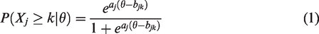
In these equations, θ represents the latent score of a respondent on the metric of the instrument, a_j determines the rate of increase of the logistic curves, and b_jk is the location on the metric of the instrument where respondents have a probability of 0.50 of choosing category k or higher. Parameters a_j and b_jk are conventionally called “slope” (or “discrimination”) and “threshold” (or “difficulty”) parameters, respectively.¹⁰ Since the latent score θ is unobservable, the metric of the instrument is not defined by the model, but must be identified using model constraints. In most cases, the GRM is estimated using marginal maximum likelihood (MML),^11,12 where the scale is fixed using a latent density function $g (θ)$ in which the mean and variance are constrained. Conventionally, $g (θ)$ is assumed to be the standard normal density (a mean of zero and a standard deviation of one).

Following the initial applications of IRT in health outcomes research, challenges of this new venue were identified.¹³ One of these challenges is related to the nature of the variables of interest and the assumption of standard normality of the latent score distribution (shown in Figure 1, left-hand panel). In health outcomes research, constructs are often operationalized in such a way that there is a lower end of the scale which merely expresses the absence of the underlying construct (e.g., “no depression”) and a higher end which expresses severity using a substantially finer gradation (e.g., “mild,” “moderate,” or “severe” depression). Such constructs are called “quasi-traits,”¹³ and one of their characteristics is that the underlying latent variable may be non-normally distributed in the population used for calibrating the instrument.

Figure 1.

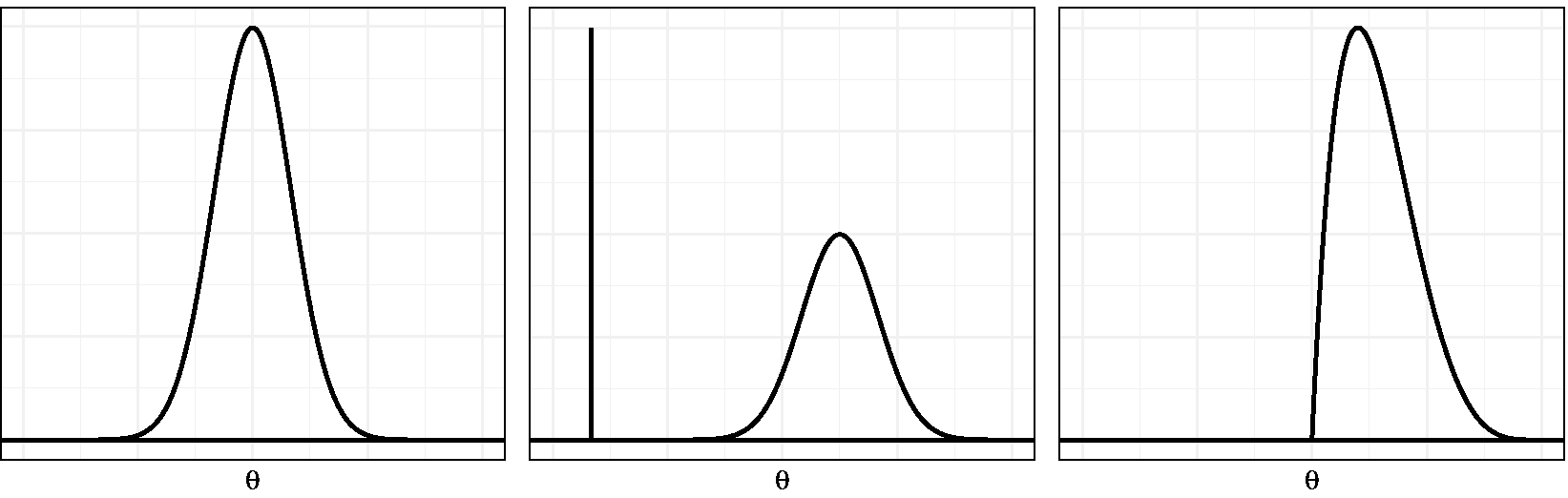
Normal, zero-inflated, and skewed latent trait distribution examples.

The non-normality of quasi-traits may be the consequence of various processes.^14–16 First, the population may be composed of two or more subpopulations. For instance, the general population may be composed of individuals with and without depression. Then one could assume a normal distribution for each subpopulation, allowing for differences in severity between populations, like in a multiple-group model.¹⁷ However, in the case of quasi-traits, with all respondents from the healthy group selecting the lowest response options, it is not realistic to assume normality within each group. In fact, a latent score cannot be assigned to respondents from this population, since a complete zero pattern does not contain information about the specific latent score. One way to deal with this is to assume an additional response process leading to the surplus of zero-patterns. More specifically, a normal distribution for the latent variable has been suggested for the regular response process and a constant distribution for the latent variable under the other response process. For example, when measuring depression severity, a normal distribution is assumed for the subpopulation suffering from depression, and the healthy subpopulation would be assumed to have a very low latent trait score with no variance (Figure 1, middle panel). This scenario has been referred to as “zero-inflation,” since there is an excess of complete zero patterns under the IRT model.^7,16 An alternative scenario leading to non-normality would be one where the latent trait distribution in the population is skewed (Figure 1, right-hand panel). This situation may arise when the majority of the population has low to medium latent trait scores but a small fraction with much higher scores is also present.¹⁸ This process will be referred to as “skewness.”

Previous research suggests that the violation of the normality assumption is detrimental to item parameter and score estimates. For instance, a study examining the robustness of MML estimation of the Rasch model revealed that deviations from normality caused bias in item parameter estimates, with bias increasing with more severe skewness.¹⁹ Another study suggested that when the underlying distribution is positively skewed, assuming a normal distribution would introduce negative bias in slope estimates and negative bias for lower category threshold estimates, which means that the estimates would be too low.¹⁵ In addition, the bias in parameter estimates has been shown to be more outspoken for extreme values of the parameter.²⁰ Recently, similar results were reported,²¹ although one study reported smaller biases.²² It has also been suggested that parameter estimates are biased in the presence of zero-inflation;^16,23 for instance, the slope parameters would be overestimated. Biased parameter estimates may lead to biased latent score estimates, by which conclusions with reference to a patient’s relative standing or a patient’s progress may be false.²⁴ Also, biased parameter estimates may lead to biased estimates of reliability, by which the measurement precision of a patient’s score estimate may be under- or overestimated.¹⁷

To deal with the bias stemming from non-normality, alternative IRT models have been developed. Recently, the use of mixtures of normal distributions was suggested as an approximation to non-normal distributions.²⁵ A special case of the mixtures of normal distributions can be used when zero-inflation is expected and is called zero-inflated mixture IRT (ZIM-IRT).^16,23 Also, solutions have been suggested for estimating IRT models for data resulting from skewed latent distributions, such as incorporating a skewed-normal density,²⁶ and augmenting the model with an extra step in which the density is estimated empirically. Two recent examples of the latter approach are Ramsay Curve IRT (RC-IRT)¹⁵ and Davidian Curve IRT (DC-IRT).²⁷

Recently, the use of ZIM-IRT and RC-IRT, among others, was exemplified using the PROMIS Anger item bank,²⁸ which consists of 29 polytomous items. The authors reported that, in comparison to the GRM, the slope estimates were higher for RC-IRT and lower for ZIM-IRT, whereas the threshold estimates had a smaller range for RC-IRT and a larger range for ZIM-IRT. This study was illustrative of the considerable impact of model choice on item parameters. However, because it used empirical data, which obviously lack an unequivocal criterion (e.g., true values of item parameters), the relative performance of the competing approaches could not be assessed. For a systematical and objective comparison of methods, Monte Carlo simulations are more appropriate.

Several simulation studies have shown promising results for methods dealing with non-normality, but the conditions under which these methods were evaluated were not in line with the settings commonly encountered while developing item banks for health outcomes. For instance, ZIM-IRT was evaluated using simulated data sets which consisted of 10 or 11 items with dichotomous response options,^16,23 whereas the PROMIS item banks, for instance, typically contain many more items and more than two response options.²⁹ Likewise, the parameter recovery performance of DC-IRT has not yet been evaluated in a simulation study where polytomous items are considered. Therefore, the available series of simulation studies is incomplete, and additional studies are required to examine the performance of these new methods in settings typical for health outcome measurement.

The aim of the current study was to investigate two models, each corresponding to one of the possible causes of non-normality discussed previously, focusing on the settings typically encountered in the assessment of health outcomes, where the measured constructs often consist of quasi-traits and the item pool commonly consists of a large number of polytomous questions. The method for tackling non-normality caused by zero-inflation, ZIM-IRT, is the most popular method in the literature. The method for dealing with skewness, DC-IRT, is the simplest method available allowing for flexible estimation of various forms of the latent distribution, including skewed distributions. Moreover, both methods are readily available in popular software packages, ZIM-IRT in Mplus¹¹ and DC-IRT in the R package mirt.¹² Polytomous extensions of ZIM-IRT and DC-IRT were compared to the GRM, in order to identify the conditions under which these models improve parameter estimation.

Methods

Models for non-normal latent trait distributions

The first method that was examined was the ZIM-GRM, which is the extension of ZIM-IRT²³ to deal with zero-inflation in polytomous items. ZIM-IRT was inspired by the models developed for dealing with excess zeros in count data with correlated observations³⁰ and combines the idea of using latent classes to identify a group with extreme responses with a method for weakening the normality assumption through a mixture distribution.²³ ZIM-GRM replaces the standard normal density used in MML estimation with a mixture of distributions

f (θ) = π I (θ = - 100) + (1 - π) g (θ)

(3)

The first term (where I is an indicator function) states that with probability π, the latent trait is assigned a score of −100, and the second term (where g represents a normal density) states that with probability $1 - π$ , the latent trait is normally distributed. Parameter π is the proportion of respondents in the population who belong to the zero-inflation state. As such, $f (θ)$ represents a mixture distribution of a normal and a degenerate component.³⁰ Alternatively, the model may also be explained through a latent class model.¹⁶ It contains two latent classes, the first class being represented by a normal latent trait distribution and the zero-inflation class by a degenerate distribution for $θ = - 100$ .

The second method was the DC-GRM, the extension of DC-IRT²⁷ for polytomous items. DC-GRM modifies the standard normal density used in estimation of the GRM, $g (θ)$ , with a Davidian curve (a semi-nonparametric method for approximating densities³¹) which is given by

h (θ) = R_{t}^{2} (θ) g (θ)

(4)where g represents a normal density, t is the number of smoothing parameters, and the term

R_{t} (θ) = \sum_{λ}^{t} m_{λ} θ^{λ}

is used for relaxing normality, where

m = (m_{0}, m_{1}, \dots, m_{t})

is the vector of smoothing parameters and

m_{t} \neq 0

. Since R_t is a polynomial of degree t, higher values of t makes the density more flexible. During model estimation,

h (θ)

is constrained to have a zero mean and unit variance to maintain the GRM’s usual scale.^27,31 Under these constraints, t = 0 and t = 1 give the standard normal density. During the analysis, the best fitting t is chosen among a set of candidates. Lower values of the Hannan–Quinn information criterion (HQC),³² which is a function of the model’s likelihood, number of parameters, and sample size, have been suggested for model selection.²⁷ In the current study, DC-GRMs were estimated using

t = 2, 3, 4, 5

. The model with the smallest HQC was selected for obtaining item parameter estimates.

Finally, to illustrate the impact of ignoring non-normality and to provide a benchmark for the new methods, the standard version of the GRM was examined as well.

Simulation design

In the simulation study, the following four factors were varied: number of respondents, number of items, ratio of zero-respondents, and skewness of the latent score distribution. The levels of these factors were based on a review of the literature, as described below.

Regarding the number of respondents, simulation studies have suggested to use a sample of at least 500 observations for estimating the GRM with sufficient precision,³³ but is common in health outcome research to use larger samples for calibration,^1,34 and therefore, levels of 500 and 1000 respondents were used.

Regarding the number of items, calibration studies in the health outcomes field have been published with number of items ranging from 10 to 124 items;²⁹ to cover a large part of this range, levels of 5, 25, and 50 were used.

The levels of rate of respondents in the zero-inflation group were fixed at 0%, 10%, and 25% to include the absence of zero-inflation, a ratio representative of published studies,^18,28 and a ratio closer to extreme cases in the literature, respectively.^16,23

Since no calibration studies were found that reported on the estimated skewness of the latent trait, skewness levels were based on the range encountered in previous simulation studies^19,20,22; levels of skewness of 0, 0.50, and 0.75 were used.

Because in the simulation study two separate scenarios for causing non-normality were examined, its design had a hierachical nature. The factors number of respondents and number of items were nested within factor rate of zero-inflation and within factor skewness, producing a $2 \times 3 \times 3$ design for each scenario; within each design cell, 100 replications were produced yielding a total of 1800 + 1800 = 3600 simulated data sets.

Data generation

Although it is common in simulation studies to use parameter values typically encountered in the field of interest,^35,36 it was chosen not to use calibration results from the health outcomes field, as many studies^1,18,37,38 show signs of non-normality themselves which likely resulted in biased parameter estimates. By contrast, it was chosen to use parameter values from a classic simulation study using the GRM,³³ in which the values for item parameters of a “good” test were specified. Discrimination parameters were drawn from a uniform distribution between 0.75 and 1.33, and threshold parameters were drawn as follows: b₁ uniform between −2.0 and −1.0, b₂ uniform between −1.0 and 0.0, b₃ uniform between 0.0 and 1.0, and b₄ uniform between 1.0 and 2.0. For each data set, a new draw was taken from these distributions, by which the true item parameter values varied over replications.

For each data set, two subsets were created. The first was a “calibration set” for studying the impact of non-normality on the item parameter estimates of the various methods. The second was a “validation set” which was used to illustrate the impact of potential deviations in the estimation of item parameter on estimates of the latent trait score. For the calibration sets, the latent trait scores were created as follows. Under the skewness scenario, the method introduced by Fleishman³⁹ was used to provide the skewed latent trait distribution with a mean of zero and standard deviation of one. Under the zero-inflation scenario, the non-zero-inflated part of the latent trait distribution followed a standard normal distribution. The zero-inflation part consisted of latent trait scores of −100, and the rate of zero-inflation was varied by varying the fraction of respondents drawn from the zero-inflated part. For all validation sets, 51 true latent score values between −2.5 and 2.5 with increments of 0.1 were used.

In the creation of each data set, using the sampled values of item parameters and latent trait scores, equations (1) and (2) were used to calculate the five response category probabilities of each item for each simulated respondent. Next, item responses were obtained by randomly drawing from the resulting multinomial distributions. If not all five item categories were observed for all items in the calibration set, item parameters were re-sampled and item responses were created anew.

Simulation outcomes

Of each data file, the calibration set was used to examine item parameter estimates, and the validation set was used to examine latent trait scores. Although other methods are available for estimating latent traits,⁴⁰ it was chosen to use maximum likelihood (ML) in order to keep the estimation in agreement with the modeling approach.

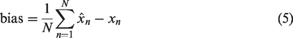
The primary outcome of the simulation study was the bias of both item and person parameter estimates, which was calculated as the mean difference between the true values and estimates

bias = \frac{1}{N} \sum_{n = 1}^{N} {\hat{x}}_{n} - x_{n}

(5)where x_n and

{\hat{x}}_{n}

are the true parameter value, and the estimate of the parameter, respectively, and N is the total number of values used for aggregation. N differs for item and person parameters: for latent trait values (e.g.,

θ = - 1.5

), N is equal to the number of replications (100), whereas for each of the five item parameters (e.g., the a-parameter), N is equal to

J \times 100

as the outcomes are aggregated across all items within a data set. Note that since true item parameter values vary within data sets and over replications, like

{\hat{x}}_{n}

, x_n is expected to vary. Bias will be larger than zero when the parameters are systematically overestimated, equal to zero if estimates are on average equal to the true value and smaller than zero if parameters are underestimated.

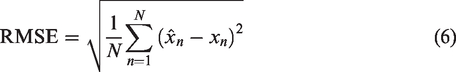
As secondary outcome measure, the root mean squared error (RMSE) was used, which was calculated as

RMSE = \sqrt{\frac{1}{N} \sum_{n = 1}^{N} {({\hat{x}}_{n} - x_{n})}^{2}}

(6)and which is a function of both bias and sampling variance;⁴¹ it was chosen to report on this outcome only when it provided information over and above the bias measure.

Data analysis

For analyzing the impact of non-normality on item parameters, both tabulations and graphical displays of the average bias and RMSE in each cell of the design were used. For analyzing the impact on latent trait estimates, graphical displays depicting the outcomes as a function of true latent values were used.

For the simulation and data analysis, R (version 3.5.1)⁴² was used. The R packages mirt (version 1.29)¹² and SimDesign (version 1.13)⁴³ were used for generating data, estimating GRM and DC-GRM, and managing simulations. DC-GRM estimation was implemented as part of the mirt package during the study (see Appendix A for details of the implementation). The ZIM-GRM was estimated using the MplusAutomation package (version 0.7.3)⁴⁴ for running Mplus version 7.4 from R.¹¹ The original Mplus script published by Wall et al.²³ for dichotomous item responses was adapted for the current settings.

Results

Throughout the analyses, the outcomes for sample sizes of 500 and 1000 were highly similar. Therefore, in this section, we mainly focus on results for the condition with 500 respondents and only discuss the condition with 1000 respondents when results clearly deviate. Tables 1 to 4 and 6 to 9 in Appendix B provide detailed results for both levels of sample size. Also, as the secondary outcome measure RMSE provided no additional information compared to the bias it was decided to leave it out of the report.

Zero-inflated latent trait distributions

A first inspection of the ZIM-GRM results showed that the estimate of the rate of zero-inflation (π in equation (3)) was very close to the true rate: in all conditions with 25 and 50 items, for every data set, the estimates were within 0.2 and 0.1 percentages points of the true values, respectively. In the five-item condition, estimates were always within two percentage points of the true value.

Figure 2 shows the average bias in the estimation of the a, b₁, and b₄ parameter as a function of number of items and rate of zero-inflation for both the GRM and ZIM-GRM. In the absence of zero-inflation (see the left-hand panel of each of the three plots), both the GRM and the ZIM-GRM had an average bias close to zero for all levels of number of items. In the zero-inflation conditions, whereas the ZIM-GRM mostly showed unbiased parameter estimates, the GRM showed substantial bias, with bias increasing with increasing zero-inflation and increasing number of items. In the case of 10% zero-inflation, the average bias in a parameter estimates was 0.54, 0.80, and 0.98, respectively, for numbers of items of 5, 25, and 50; in the case of 25% zero-inflation, these values were more than twice as high. Parameter b₁ showed a similar pattern: in the 10% zero-inflation condition, the average bias was 0.75, 0.92, and 1.01, respectively, for numbers of items of 5, 25, and 50; in the 25% zero-inflation condition, these respective values were at least 60% higher. The b₄ parameter showed an opposite but less extreme pattern: it was somewhat overestimated with less bias for lower numbers of items, and with differences between the rate of zero-inflation conditions that were much smaller. Turning to the GRM estimates of parameters b₂ and b₃ (see Table 1 in Appendix B), average bias showed a similar pattern as for b₁, but bias was smaller with b₃ showing considerably less bias than b₂. In short, in case of zero-inflation, the GRM overestimated the a parameter, and it yielded b parameters with both a biased center (estimates were too high) and a biased spread (the estimates of the respective thresholds were too close to one another).

Figure 2.

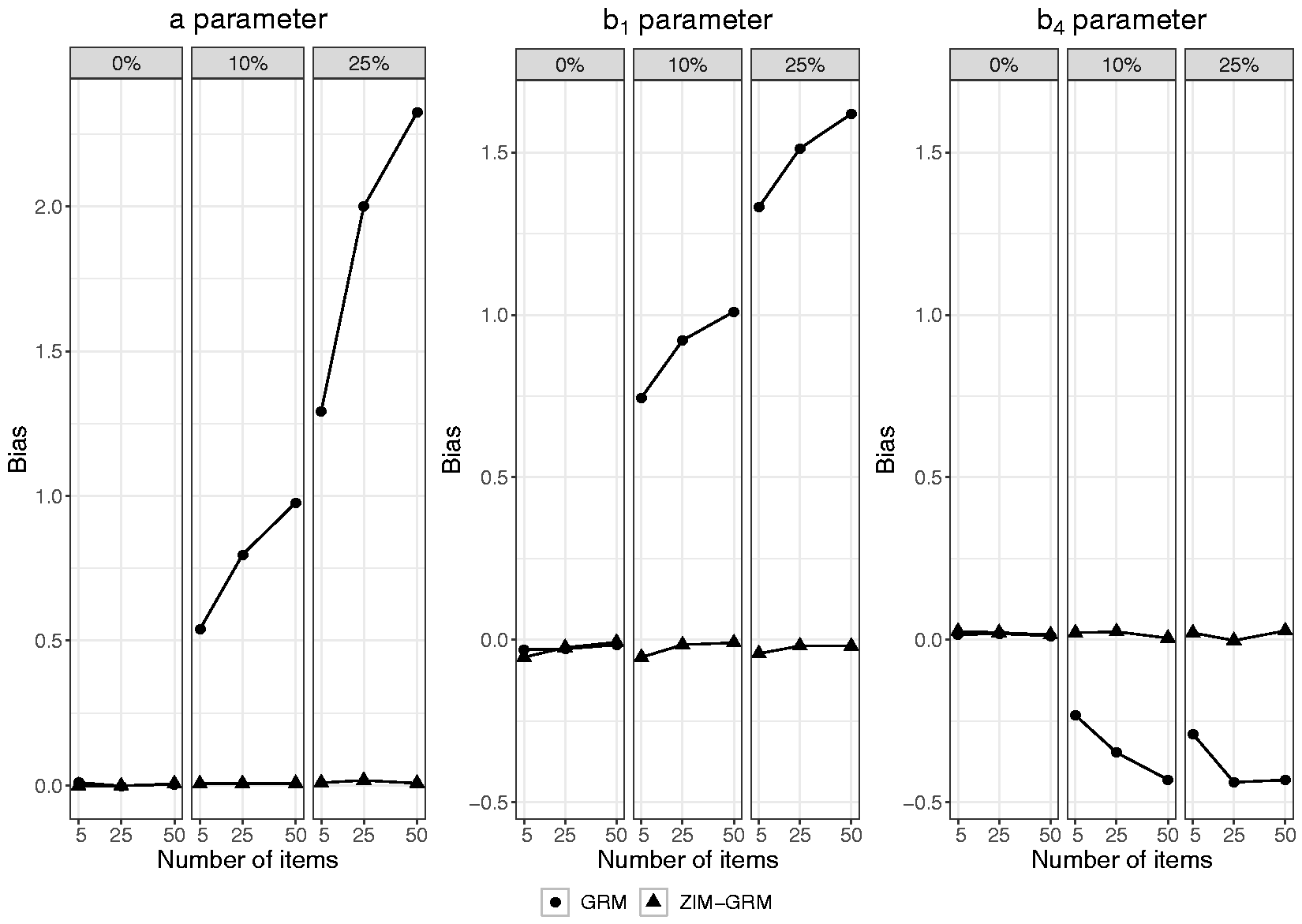
Bias in item parameter estimates of the GRM and ZIM-GRM per level of number of items and of zero-inflation (0%, 10%, and 25%) for a sample size of 500. GRM: graded response model; ZIM-GRM: zero-inflated mixture graded response model.

Figure 3 shows the average bias in the estimation of the latent score as a function of true latent score, number of items, and rate of zero-inflation for both the GRM and ZIM-GRM (also see Tables 3 and 4 in Appendix B, for average bias values of aggregated values of the true latent trait). In the absence of zero-inflation (see the data points depicted by a square), both the GRM and ZIM-GRM showed no bias except for true latent scores smaller than −2 (small positive bias) and larger than 2 (small negative bias) in case of a number of items of five. This is an artifact originating from the use of ML for estimating the latent scores: for these regions, extreme response patterns (0 0 0 0 0, and 4 4 4 4 4, respectively) were frequently encountered, and ML’s inability to scale these resulted in missing values, which were excluded from the analysis. As a result, the average estimate for the remaining response patterns of high (low) true latent scores were artificially low (high). In the two zero-inflation conditions, whereas the ZIM-GRM showed unbiased latent score estimates, the GRM showed substantial bias, with bias increasing with increasing zero-inflation and increasing number of items. For example, in the case of five items and 10% zero-inflation, a true value of −2.5 was overestimated by more than one unit. The plots show that both the spread and center of the latent scale were affected by the GRM: For more extreme true latent scores, estimates were more biased toward zero, but the size of shrinkage was larger on the left-hand side of the scale than on its right-hand side, yielding a positively valued overall average bias.

Figure 3.

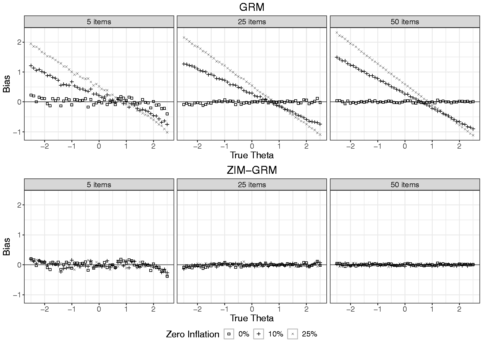
Bias in latent trait estimates for the GRM and ZIM-GRM per level of number of items and zero-inflation for a sample size of 500. GRM: graded response model; ZIM-GRM: zero-inflated mixture graded response model.

Skewed latent trait distributions

As DC-IRT was not yet available in publicly available software, it was implemented as part of the mirt package during the study. Appendix A shows a validation study in which the simulation results of the original procedure by Woods and Lin²⁷ were successfully replicated.

In a first inspection of the estimated DC-GRMs, the number of selected smoothing parameters (t in equation (4)) was examined (see Table 5 in Appendix B, which shows its average for each cell of the simulation design). When skewness was absent, the average number of selected smoothing parameters was very close to the minimally required number of two parameters for all conditions. When skewness was present, t increased (indicating responsiveness to non-normality) with increasing skewness and increasing number of items; this pattern applied to both numbers of respondents, but with somewhat higher values in the condition with 1000 respondents.

Figure 4 presents the average bias in the estimates of a, b₁, and b₄ as a function of number of items and level of skewness for both the GRM and DC-GRM. In the absence of skewness (see the left-hand panel of each of the three plots), the GRM and DC-GRM had very similar outcomes, with average bias within 0.02 of each other and no values exceeding 0.04 in absolute value. In the two conditions with skewed latent traits (a skewness of 0.50, and 0.75, respectively), the GRM and DC-GRM mostly showed similar outcomes as well, both with average bias very close to zero for the a parameter, and for the b parameters mostly values within 0.03 of each other, and most values not exceeding 0.05, with the exception of the estimates of b₄. For this parameter, whereas for five items, the average bias of the DC-GRM was very close to zero, for 25 and 50 items, its average bias was somewhat higher (0.06 and 0.08, respectively) than that of the GRM (0.02 and 0.03, respectively); for both methods, however, this bias was lower in the case of 1000 observations. In short, whereas the GRM was hardly affected in the two conditions with skewed latent traits, the DC-GRM showed a small bias in conditions with the highest level of skewness and the largest studied item set. To illustrate the effect of bias in item parameters on latent trait estimates, Figure 5 shows the average bias in latent trait estimates as a function of true latent score, level of skewness, and number of items for both the GRM and DC-GRM (also see Tables 8 and 9 in Appendix B, for the average bias of aggregated values of the true latent trait). In the absence of skewness (see the data points depicted by a square), both the GRM and DC-GRM showed no bias except for extreme true latent scores, an artifact due to using ML for estimating latent scores, as described in the previous section. In the presence of skewness, the results of the GRM and DC-GRM were mostly very similar, showing little bias, with the exception of the condition with a skewness of 0.75 and 50 items, in which the DC-GRM showed somewhat more extreme bias than the GRM, with the highest mean difference between the methods being 0.07 for trait scores above 1.5.

Figure 4.

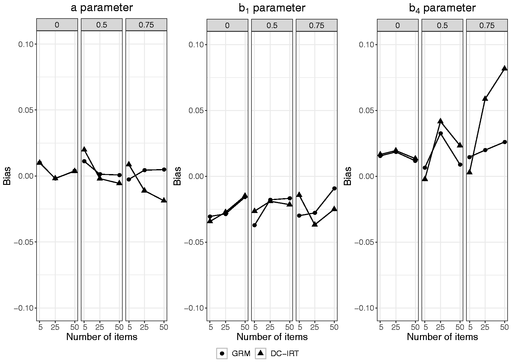
Bias in item parameter estimates of the GRM and DC-GRM per level of number of items and of skewness (0, 0.50, and 0.75) for a sample size of 500. GRM: graded response model; DC-GRM: Davidian curve graded response model.

Figure 5.

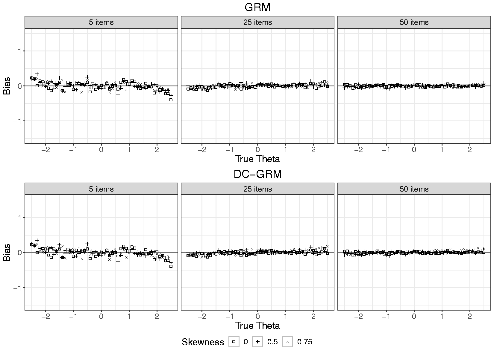
Bias in latent trait estimates for the GRM and DC-GRM per level of number of items and skewness for a sample size of 500. GRM: graded response model; DC-GRM: Davidian curve graded response model.

Discussion

In the current study, two IRT models for polytomous items designed to deal with two different processes leading to non-normally distributed latent traits were evaluated. The ZIM-GRM was used to deal with zero-inflation, and the DC-GRM was used to deal with skewness. Both methods were compared with the standard GRM in a simulation study with conditions representative of the settings, wherein IRT is commonly used to develop item banks for health outcomes. The impact of the simulation conditions was assessed for both item parameter estimates and latent trait estimates.

In the case of zero-inflated latent trait distributions, the GRM showed substantial bias, with larger bias for distributions with a higher rate of zero-inflation, and for larger number of items, whereas the ZIM-GRM showed very little bias. The GRM overestimated the a parameter to a high extent and resulted in b parameters that were too high, with the exception of the highest threshold, which was somewhat underestimated; moreover, the estimates of the respective thresholds were too close to one another. The latent trait estimates of the GRM showed a similar pattern, largely overestimating low latent trait values, and somewhat underestimating high values. Although the conditions and outcomes are not directly comparable, some of the current outcomes were in line with those of the simulation study by Wall et al.²³ for binary items. First, in the binary case, zero-inflation was also associated with overestimating the discrimination parameter. Second, the pattern within polytomous items (of showing an overestimation of the center and a decrease in the spread of the scale) was also present over the collection of binary items in that thresholds were overestimated on average with more overestimation for low thresholds than underestimation for high thresholds.

In the case of skewed latent trait distributions, whereas the GRM mostly showed no bias, the DC-GRM showed a small bias with both high skewness and large item sets. In other words, the GRM outperformed its extension, the DC-GRM, which was included in the study to deal with skewness. This is not in line with previous research which suggested that ignoring skewness causes bias, although the size of bias varies across studies.^15,19–22 This discrepancy may have emerged from the method used for creating skewed distributions. Whereas we used the method by Fleishman³⁹ which resulted in distributions with zero kurtosis, the studies by Woods¹⁵ and Woods and Lin,²⁷ for example, used mixtures of normals, which resulted in substantial kurtosis. Evidently, a distribution with skewness only is more easily approximated by a normal distribution than one with both skewness and kurtosis. The plausibility of this explanation is supported by the current outcomes being more similar to those of a study using a more similar method for generating skewness²² than to those of a study using a different method for generating skewness.¹⁵ The somewhat biased results of the DC-GRM may have resulted from the way it was implemented here. Inspection of the number of smoothing parameters (see Table 5) shows that the highest values were selected in the conditions with the highest deviations in parameter estimates, which suggests that the method may have suffered from overfitting.⁴⁵ The choice for using HQC for model selection was based on the recommendations from the simulation study that examined DC-IRT for dichotomous items,²⁷ but possibly this index is not optimal in the case of polytomous items; it is advised that future research compares the index with more conservative indices like the Bayesian information criterion.

In their classic article on quasi-traits in clinical measurement, Reise and Waller⁴⁶ suggested that high discrimination parameter estimates originated from conceptually narrow constructs and consequently homogeneous item content leading to highly correlated items. For unipolar and skewed constructs, they are correct that improper latent trait shapes are selected and therefore that the resulting parameters may be on a suboptimal scale. However, concerning the bias that arises when using the GRM in case of zero-inflation, it may be claimed that the outcome is both good and bad. It is bad because in reality the items do not discriminate as much among respondents as the parameter estimates suggest. By contrast, it is good because the GRM does not change the ordering of the respondents (see Figure 3, which shows a linear transformation), and because it becomes very efficient at discriminating between the clinical and non-clinical respondents. Thus, the mixing of samples results in a “population discrimination” item-level artifact rather than the originally desired “person discrimination” goal of the IRT measurement model.

For future studies on zero-inflation, it may be instructive to discuss the impact of the degenerate part of ZIM-IRT on simulation results. In the current and previous evaluations²³ of ZIM-IRT, the model specification was perfectly in line with the data generating process, both using a mean of zero and a standard deviation of one for the non-degenerate component, and a mean equal to an extreme negative value and a variance of zero in the degenerate component. However, when a model is specified in any other way, the scale of estimated item and person parameters will, by definition, be different than the data generating scale, resulting in artificially biased outcomes. For example, when using DC-IRT for estimating the zero-inflated distribution, the estimation algorithm tries to pick up its shape, including both mixtures in a single smooth curve while constraining the distribution to have a mean of zero and a standard deviation of one, which will lead to failure because it is mathematically impossible to include both the zero-inflated part and the proper scale for non-zero-inflated part in a single distribution.¹ In such cases, since the scales are incompatible, a solution would be to use the correlation between true and estimated parameters as outcome, instead of exploring bias or RMSE.

In the current study, we focused on methods available in software, which is possibly only a small selection of the methods that have been proposed to deal with non-normality. In the case of skewness, several other methods have been developed,^26,47,48 and an examination of their performance in the current conditions may seem interesting, but the negligible bias that was observed for GRM reduces its necessity. In the case of ZIM-IRT, the studied approach can be easily extended to not only deal with zero-inflation but also with maximum-inflation (an excess of patterns containing only the highest item category for each item).^16,23 More recently, similar approaches have been taken for questionnaires that include items eliciting count responses that suffer from heaping (an excess of patterns with multiples of 5 in reporting days of having experienced a specific symptom).^49,50 These methods are characterized by modeling extreme response patterns by specifying one or more classes with a degenerate distribution, which may be difficult to interpret for practitioners, and therefore, it seems appropriate to look at other approaches to mixture modeling as well.² It is also noted that other types of IRT models have been developed for explicitly dealing with extreme response behavior,^51,52 and finally, it is acknowledged that methods for dealing with other deviations from normality, such as unipolar traits,^50,53 are available. It is recommended that future research examines the usefulness of such methods in the calibration of item banks for measuring health outcomes.

When comparing the parameter estimates of the standard GRM under both zero-inflation and skewness, it was striking that the values of the former were very similar to what is commonly encountered in calibration studies of health outcome item banks. For example, like in most studies,^1,18,37,38 in case of zero-inflation, the standard GRM produced very high estimates of discrimination parameters and threshold estimates that were mainly located at the positive side of the latent trait scale. Given that in many calibration studies, excessive zeros were reported and that the parameter estimates were so similar, it seems plausible that the true data generation process is similar to the one that we used for creating zero-inflation. This would imply that using the standard GRM for calibrating health outcome item banks leads to biased parameter estimates. Overestimation of discrimination parameters leads to standard errors of latent trait estimates that are too optimistic,⁵⁴ which in computerized adaptive testing could lead to assessments that stop too early. Moreover, if one blindly interprets the latent trait estimates under the metric of the standard normal distribution (e.g., using percentile ranks), then respondents may seem to score less extreme than they actually do. Therefore, when calibrating item banks for the assessment of health outcomes, it seems like a good practice to consider the possibility of subpopulations. Although calibration samples often consist of commingled populations,¹⁷ such as a clinical and non-clinical population, it is often hard to determine for the individual respondent to what population she belongs, which does not allow for a multi-group approach.⁵⁵ However, when using the ZIM-GRM, instead of (potentially incorrectly) assigning each individual to a subpopulation prior to fitting the GRM, the uncertainty is built into the model directly, where individuals are assigned probabilistically rather than deterministically. The appropriateness of the ZIM-GRM compared to the GRM for calibration data can be evaluated using model fit indices.²³

Footnotes

Acknowledgements

We thank Carol Woods and Scott Monroe for their scholarly correspondence to our questions regarding their software implementation. Part of the simulations presented in this paper was carried out on the Dutch national e-infrastructure with the support of SURF Cooperative.

Declaration of conflicting interests

The author(s) declared no potential conflicts of interest with respect to the research, authorship, and/or publication of this article.

Funding

The author(s) received no financial support for the research, authorship, and/or publication of this article.

ORCID iDs

Niels Smits

Oğuzhan Öğreden

Mauricio Garnier-Villarreal

Notes

References

Pilkonis

Choi

Reise

, et al. Item banks for measuring emotional distress from the Patient-Reported Outcomes Measurement Information System (PROMIS®): depression, anxiety, and anger. Assessment 2011; 18: 263–283.

Samejima

Estimation of latent ability using a pattern of graded responses. Psychom Monogr 1969; 17: 1–100.

Van Der Linden

Hambleton

RK.

Handbook of modern item response theory. Berlin: Springer Science & Business Media, 2013.

Edelen

Reeve

BB.

Applying item response theory (IRT) modeling to questionnaire development, evaluation, and refinement. Qual Life Res 2007; 16: 5–18.

Ader

DN.

Developing the Patient-Reported Outcomes Measurement Information System (PROMIS). Med Care 2007; 45: S3–S11.

Saha

Chou

Grant

BF.

Toward an alcohol use disorder continuum using item response theory: results from the National Epidemiologic Survey on Alcohol and Related Conditions.

Psychol Med 2006; 36: 931–941.

Aggen

Neale

Kendler

KS.

DSM criteria for major depression: evaluating symptom patterns using latent-trait item response models.

Psychol Med 2005; 35: 475–487.

Emons

Meijer

Denollet

Negative affectivity and social inhibition in cardiovascular disease: evaluating type-D personality and its assessment using item response theory.

J Psychosom Res 2007; 63: 27–39.

Reeve

Hays

Bjorner

, et al. Psychometric evaluation and calibration of health-related quality of life item banks: plans for the Patient-Reported Outcomes Measurement Information System (PROMIS). Med Care 2007; 45: S22–S31.

10.

Ayala

RJD.

The theory and practice of item response theory. New York: Guilford Press, 2009.

11.

Muthén

Mplus user’s guide. 7th ed. Los Angeles: Muthén & Muthén, 2012.

12.

Chalmers

RP.

Mirt: a multidimensional item response theory package for the R environment. J Stat Softw 2012; 48: 1–29.

13.

Reise

Waller

NG.

Item response theory and clinical measurement.

Ann Rev Clin Psychol 2009; 5: 27–48.

14.

Reise

Revicki

DA.

Introduction: age-old problems and modern solutions. In: Handbook of item response theory modeling. Abingdon: Routledge, 2014, pp. 21–30.

15.

Woods

CM.

Ramsay-curve item response theory (RC-IRT) to detect and correct for nonnormal latent variables.

Psychol Methods 2006; 11: 253–270.

16.

Finkelman

Green

Gruber

, et al. A zero-and K-inflated mixture model for health questionnaire data. Stat Med 2011; 30: 1028–1043.

17.

Smits

On the effect of adding clinical samples to validation studies of patient-reported outcome item banks: a simulation study.

Qual Life Res 2016; 25: 1635–1644.

18.

Amtmann

Cook

Jensen

, et al. Development of a PROMIS item bank to measure pain interference. Pain 2010; 150: 173–182.

19.

Zwinderman

Van Den Wollenberg

AL.

Robustness of marginal maximum likelihood estimation in the Rasch model. Appl Psychol Meas 1990; 14: 73–81.

20.

Boulet

JR.

The effect of nonnormal ability distributions on IRT parameter estimation using full-information and limited-information methods. Thesis, University of Ottawa, Canada, 1996.

21.

Sass

Schmitt

Walker

CM.

Estimating non-normal latent trait distributions within item response theory using true and estimated item parameters. Appl Meas Educ 2008; 21: 65–88.

22.

Rodriguez

The heteroscedastic skew graded response model: an answer to the non-normality predicament? PhD Thesis, University of California, Los Angeles, CA, 2017.

23.

Wall

Park

Moustaki

IRT modeling in the presence of zero-inflation with application to psychiatric disorder severity.

Appl Psychol Meas 2015; 39: 583–597.

24.

Zhao

Impact of IRT item misfit on score estimates and severity classifications: an examination of promis depression and pain interference item banks.

Qual Life Res 2017; 26: 555–564.

25.

Wall

Guo

Amemiya

Mixture factor analysis for approximating a nonnormally distributed continuous latent factor with continuous and dichotomous observed variables.

Multivar Behav Res 2012; 47: 276–313.

26.

Molenaar

Dolan

De Boeck

The heteroscedastic graded response model with a skewed latent trait: testing statistical and substantive hypotheses related to skewed item category functions.

Psychometrika 2012; 77: 455–478.

27.

Woods

Lin

Item response theory with estimation of the latent density using Davidian curves. Appl Psychol Meas 2009; 33: 102–117.

28.

Reise

Rodriguez

Spritzer

, et al. Alternative approaches to addressing non-normal distributions in the application of IRT models to personality measures. J Personal Assess 2017; 100: 1–12.

29.

Cella

Riley

Stone

, et al. The Patient-Reported Outcomes Measurement Information System (PROMIS) developed and tested its first wave of adult self-reported health outcome item banks: 2005s:epo. J Clin Epidemiol 2010; 63: 1179–1194.

30.

Min

Agresti

Random effect models for repeated measures of zero-inflated count data. Stat Modell 2005; 5: 1–19.

31.

Zhang

Davidian

Linear mixed models with flexible distributions of random effects for longitudinal data.

Biometrics 2001; 57: 795–802.

32.

Hannan

EJ.

Rational transfer function approximation. Stat Sci 1987; 2: 135–151.

33.

Reise

Parameter recovery in the graded response model using MULTILOG. J Educ Meas 1990; 27: 133–144.

34.

Crins

Roorda

Smits

, et al. Calibration of the Dutch-Flemish PROMIS Pain Behavior item bank in patients with chronic pain. Eur J Pain 2016; 20: 284–296.

35.

Smits

Finkelman

MD.

A comparison of computerized classification testing and computerized adaptive testing in clinical psychology. J Comput Adapt Test 2013; 1: 19–37.

36.

Edwards

Houts

Cai

A diagnostic procedure to detect departures from local independence in item response theory models.

Psychol Methods 2018; 23: 138.

37.

Rose

Bjorner

Becker

, et al. Evaluation of a preliminary physical function item bank supported the expected advantages of the Patient-Reported Outcomes Measurement Information System (PROMIS). J Clin Epidemiol 2008; 61: 17–33.

38.

Crins

MHP

Roorda

Smits

, et al. Calibration and validation of the Dutch-Flemish PROMIS pain interference item bank in patients with chronic pain. PLoS One 2015; 10: e0134094.

39.

Fleishman

AI.

A method for simulating non-normal distributions. Psychometrika 1978; 43: 521–532.

40.

Brown

Croudace

TJ.

Scoring and estimating score precision using multidimensional IRT models. In: Handbook of item response theory modeling: applications to typical performance assessment. New York: Routledge, 2014, pp. 307–333.

41.

Lindgren

BW.

Statistical theory. 4th ed. New York: Chapman & Hall, 1993.

42.

R Core Team. R: a language and environment for statistical computing. Vienna: R Foundation for Statistical Computing, 2017.

43.

Sigal

Chalmers

RP.

Play it again: teaching statistics with Monte Carlo simulation. J Stat Educ 2016; 24: 136–156.

44.

Hallquist

Wiley

JF.

MplusAutomation: an R package for facilitating large-scale latent variable analyses in Mplus.

Struct Equ Model 2011; 25: 621–638.

45.

Hastie

Tibshirani

Friedman

JH.

The elements of statistical learning: data mining, inference and prediction. 2nd ed. New York: Springer, 2009.

46.

Reise

Waller

NG.

Item response theory and clinical measurement.

Rev Clin Psychol 2009; 5: 27–48.

47.

Bock

Aitkin

Marginal maximum likelihood estimation of item parameters: application of an EM algorithm. Psychometrika 1981; 46: 443–459.

48.

Azevedo

CLN

Bolfarine

Andrade

DF.

Bayesian inference for a skew-normal irt model under the centred parameterization. Comput Stat Data Anal 2011; 55: 353–365.

49.

Magnus

Thissen

Item response modeling of multivariate count data with zero inflation, maximum inflation, and heaping. J Educ Behav Stat 2017; 42: 531–558.

50.

Magnus

Liu

A zero-inflated Box-Cox normal unipolar item response model for measuring constructs of psychopathology.

Appl Psychol Meas 2018; 42: 571–589.

51.

Bolt

Newton

JR.

Multiscale measurement of extreme response style. Educ Psychol Meas 2011; 71: 814–833.

52.

De Boeck

Partchev

IRTrees: tree-based item response models of the GLMM family. J Stat Softw 2012; 48: 1–28.

53.

Lucke

JF.

Unipolar item response models. In: Handbook of item response theory modeling: applications to typical performance assessment. New York: Routledge, 2014, pp. 272–284.

54.

Revicki

Chen

Tucker

Developing item banks for patient-reported health outcomes. In: Handbook of item response theory modeling: applications to typical performance assessment. New York: Routledge, 2014.

55.

McDonald

RP.

Test theory: a unified treatment. Mahwah: Lawrence Erlbaum, 1999.

56.

Fox

Avetisyan

van der Palen

Mixture randomized item-response modeling: a smoking behavior validation study.

Stat Med 2013; 32: 4821–4837.

A study of alternative approaches to non-normal latent trait distributions in item response theory models used for health outcome measurement

Abstract

Keywords

Introduction

Methods

Models for non-normal latent trait distributions

Simulation design

Data generation

Simulation outcomes

Data analysis

Results

Zero-inflated latent trait distributions

Skewed latent trait distributions

Discussion

Footnotes

Acknowledgements

Declaration of conflicting interests

Funding

ORCID iDs

Notes

References