
Abstract
Ultrasound growth measurements are monitored to evaluate if a fetus is growing normally compared with a defined standard chart at a specified gestational age. Using data from the Fetal Growth Longitudinal Study of the INTERGROWTH-21st project, we have modelled the longitudinal dependence of fetal head circumference, biparietal diameter, occipito-frontal diameter, abdominal circumference, and femur length using a two-stage approach. The first stage involved finding a suitable transformation of the raw fetal measurements (as the marginal distributions of ultrasound measurements were non-normal) to standardized deviations (Z-scores). In the second stage, a correlation model for a Gaussian process is fitted, yielding a correlation for any pair of observations made between 14 and 40 weeks. The correlation structure of the fetal Z-score can be used to assess whether the growth, for example, between successive measurements is satisfactory. The paper is accompanied by a Shiny application, see https://lxiao5.shinyapps.io/shinycalculator/.
1 Introduction
During pregnancy, fetal anthropometric measures consisting of head circumference (HC), biparietal diameter (BPD), occipito-frontal diameter (OFD), abdominal circumference (AC), and femur length (FL) are measured using ultrasound to monitor attained fetal size at a given gestational age (GA). By comparing measurements to a reference or standard chart,1,2 fetuses with measurements at the tails of the distribution (for example below the 3rd, 5th, or 10th centiles or above the 90th, 95th, or 97th centiles) are identified as being at increased risk of a growth disorder, such as intra-uterine growth restriction (IUGR) that may require further investigation. Growth charts, which conventionally record only cross-sectional (attained size) information, can be extended to monitor growth rate over time (velocity). 3 An assessment of the current size of the fetus in relation to the size in the past (the previous visit) enables the evaluation of an individual’s growth between any two time points (rate of growth). These changes observed between two time points may be used to identify those requiring closer monitoring. Fetal growth is rapid in the first and second trimester and slows towards term. The correlation of measurements from the same fetus is important for evaluating fetal growth velocity. The correlation coefficient is not constant as it is dependent on the interval between measurements. An estimate of the correlation coefficient is straightforward for fixed time intervals, but it is clinically useless as, in normal practice, fetuses are seen and measured at irregularly spaced time points – a model that allows for such irregularity is required. Correlation models have previously been derived for child data4–8 but not for fetal biometry data.
We model the correlation of fetal biometry (i.e. HC, BPD, OFD, AC, and FL) and derive formulae and a Shiny application that can be used to obtain the correlation for each fetal measure between measurements made at any two time points between 14 and 40 weeks of GA. We model the correlations using fetal ultrasound data from the INTERGROWTH-21st Project Fetal Growth Longitudinal Study (FGLS) on which the international standards for fetal growth are based.9,10 A separate analysis of the cohort demonstrated that the FGLS cohort remained healthy with adequate growth and motor development up to 2 years of age. 11
2 Data
The INTERGROWTH-21st Project was a population-based longitudinal study that measured serial fetal growth scans every 5±1 weeks from recruitment at 9+0 – 13+6 weeks of gestation until, but not beyond, 42+0 weeks of gestation. The FGLS component of the INTERGROWTH-21st Project is the largest prospective study to collect data on fetal ultrasound measurements from optimally healthy pregnant women to date, collecting data in eight geographically diverse populations and using many quality control measures. The FGLS involved measuring serial fetal growth scans every 5±1 weeks after the initial dating scan, so that the possible ranges after the dating scan were 14–18, 19–23, 24–28, 29–33, 34–38, and 39–42 weeks of gestation. To ensure that all sites collected high-quality data that were comparable within and between the study sites, all sonographers and anthropometrists were trained, and all ultrasound measurements were performed in a standardized manner following strict protocols. 12 All sites adopted uniform methods, used identical ultrasound equipment in all of the study sites, adopted standardized methodology to take fetal measurements, and employed locally accredited ultra-sonographers who underwent standardization training and monitoring.
The FGLS screened 13,108 pregnant women attending the study clinics
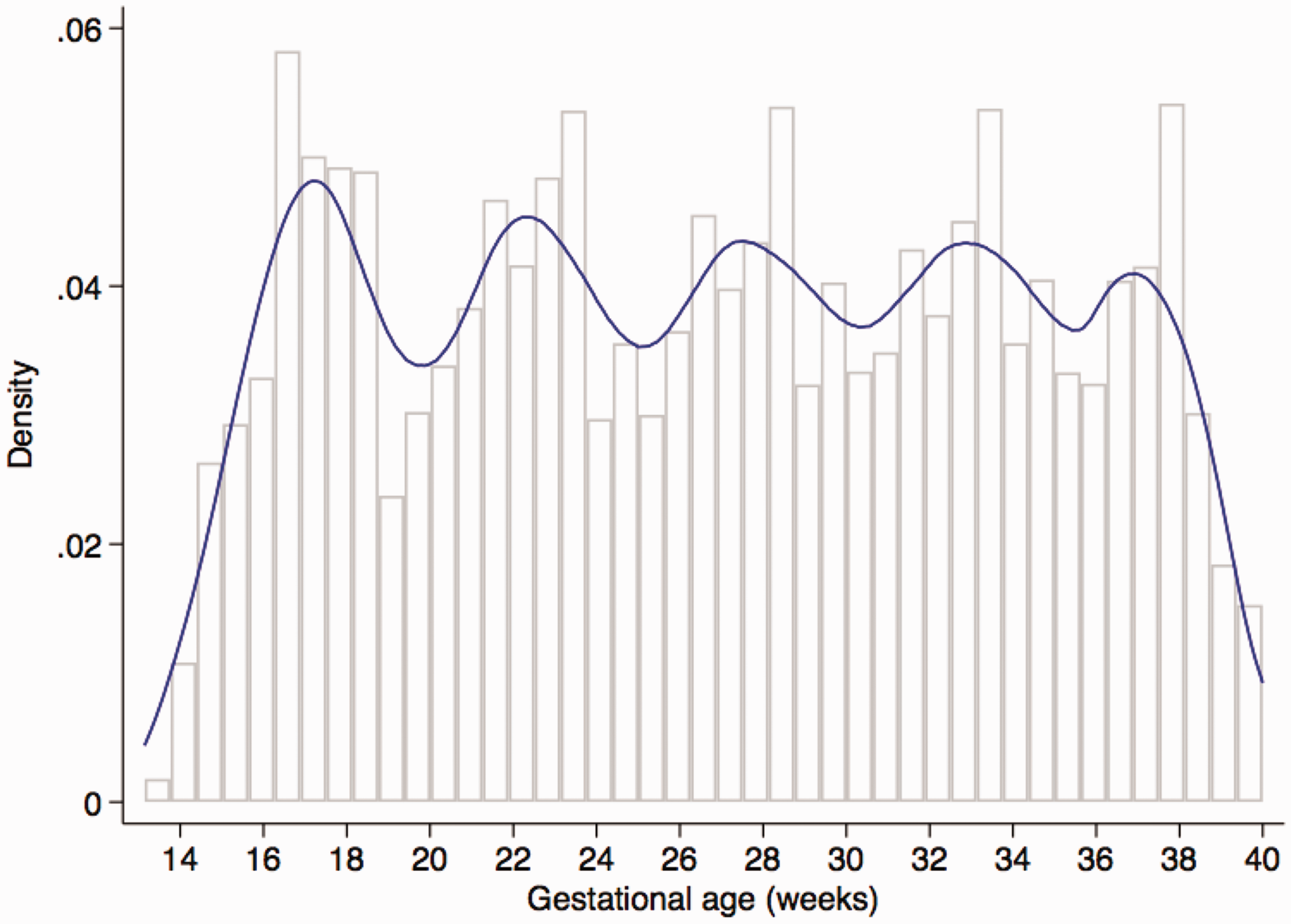
Distribution of Gestational Age at which measurements were recorded (with expected periodicity of 5 weeks).
The INTERGROWTH-21st Project was approved by the Oxfordshire Research Ethics Committee “C” (reference: 08/H0606/139), the research ethics committees of the individual participating institutions, and the corresponding regional health authorities where the project was implemented. Participants provided written consent to be involved in the study.
3 Statistical methodology
Consider the longitudinal data
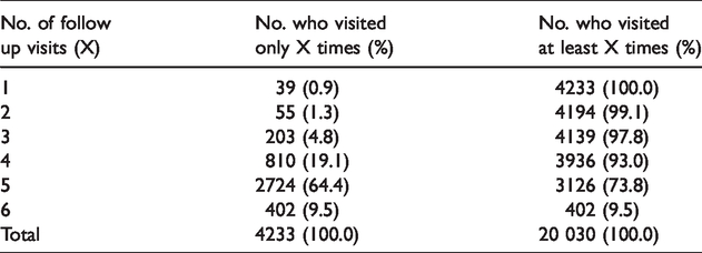
Summary of the number of women at each visit and the total number of follow-up visits.
We estimate a correlation matrix of the ultrasound measurement at different gestational ages. A single model is fitted for both sexes as some mothers do not want to know the sex of the child they expect. Because the marginal distributions of ultrasound growth measurements may be non-normal, e.g. skewed, a suitable transformation of the raw growth measurements is first identified and applied to the data to construct a working marginal reference chart. The raw fetal measurements are then transformed accordingly to provide standardized deviations (Z-scores). Next the Z-scores are modeled by a Gaussian process with zero mean and unit variance so that the temporal correlation of the process can be estimated.
3.1 Working models for marginal reference distribution
We consider the LMS transformation
17
which could transform non-normal data to make the assumption of normality acceptable. Let Y be a positive random variable and its LMS transformation is given by
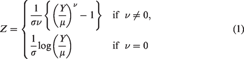
Here
We model the parameters in equation (1), 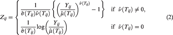
Under the BCCG model, marginally Zij has approximately a standard normal distribution. Under the BCT or the BCPE models, additional transforms of Zij are needed to make Zij normal. For simplicity, we assume all proper transformations have been applied. The Gaussian process is fully identified by its correlation matrix, which we estimate with zero mean and unit variance.
3.2 Correlation models
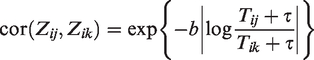
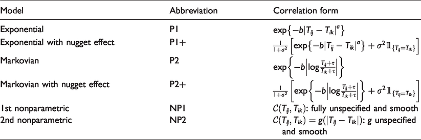
In this section, we estimate a correlation matrix for the Z-scores. We compare several parametric and nonparametric models. The parametric models considered here have been applied to child growth. The exponential model
21
(denoted by P1) is


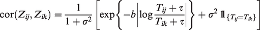
Note that with the nugget term, neither the stationary property nor the Markovian property holds.
Parametric models are simple and easy to interpret, but they can be subject to model misspecification. Thus, in addition to the above parametric correlation models, we also considered two nonparametric correlation models. The first one is based on functional data analysis,
22
which models the Z-score of a subject as the sum of a smooth random function of the gestational age and a random measurement error term. Specifically, the functional data model is

The correlation function from the functional data method is in general nonstationary. We also consider a stationary but nonparametric correlation function by assuming that the correlation function
Correlation models.
3.3 Estimation of the correlation models
The parametric correlation models are fitted by maximizing likelihood of the Z-scores under normality. We now focus on the estimation of the two nonparametric models. Estimation methods for the functional data model are well developed in the statistics literature and here we use the fast covariance estimation method for longitudinal data, developed in Xiao et al.
23
We briefly describe the method here, which will also be useful for explaining our estimation method for NP2. First, empirical estimates of the correlation function are constructed. Specifically, let
4 Results
4.1 Marginal standard charts
The estimated location, scale and skewness parameters show that a BCCG transformation model fits the data well (see Figure 2). Our empirical results also indicate that it suffices to use BCCG rather than the more complicated BCPE or BCT, as Figure 3 suggests that the estimated parameter of kurtosis is close to 2 for BCPE model and very large for BCT model. Figure 4 plots the smoothed first to fourth moments of the Z-scores against the gestational age. Specifically, nonparametric smooth functions are fitted to the data
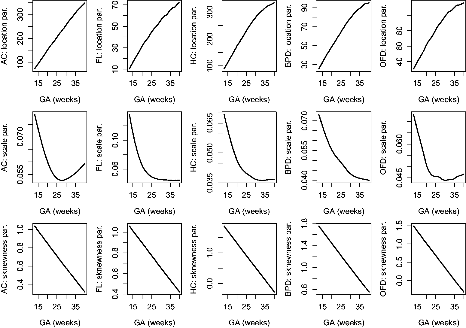
Estimated location, scale and skewness parameters as functions of gestational age for the five fetal growth measurements.
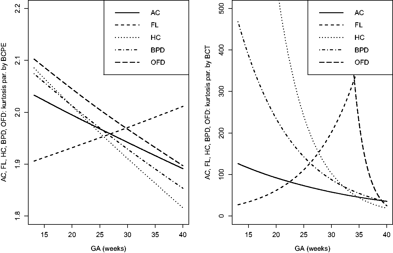
Estimated kurtosis parameters as functions of gestational age for the five fetal growth measurements using BCPE and BCT.
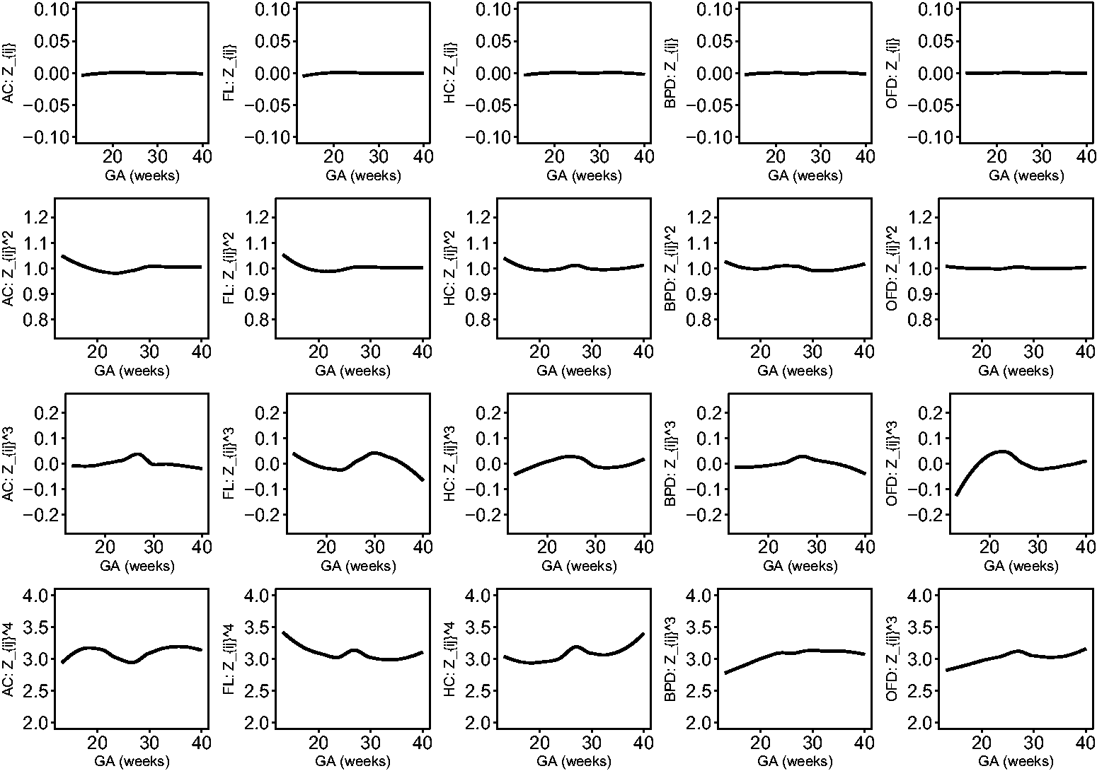
Smooth estimates of the first to fourth moments of the constructed Z-scores for AC, FL, HC, BPD and OFD.
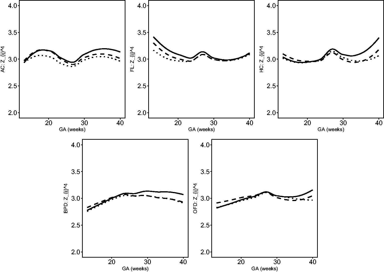
Further comparison of BCCG (solid), BCPE (dashed) and BCT (dotted) on the fourth moments of Z-scores.
Consequently, the BCCG model will be applied to construct marginal standard charts.
4.2 Correlation models
We use the BCCG model to fit the marginal distributions of the raw ultrasound measurements and then convert the transformed measurements into Z-scores. Then different parametric and nonparametric correlation models are compared via model selection criteria: AIC and BIC. Both criteria require the degrees of freedom of the model. For parametric correlation models, it is the number of free parameters. For nonparametric correlation models, the effective degrees of freedom, which evaluates the model complexity of nonparametric smoothers, 27 will be calculated.
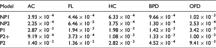
Model comparison results for AC, FL, HC, BPD, and OFD are summarized in Table 3. Table 3 shows that the P1+ model is overall the best model across the three fetal growth measurements. It fits the data best among all parametric models and has a simpler form than all the nonparametric models, and yields the smallest BIC. To quantify the differences among different correlation models, we use P1+ as the reference correlation and evaluate how the other models differ from P1+. Denote 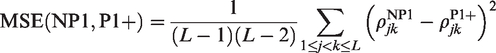
Comparison of correlation models.
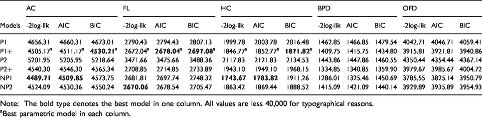
Note: The bold type denotes the best model in one column. All values are less 40,000 for typographical reasons.
aBest parametric model in each column.
Table 4 demonstrates an ignorable difference between P1+ and NP2, as expected because of the stationarity nature of both models. The difference between P1+ and NP1 is small, suggesting that an exponential correlation model with nugget effect is sufficient for fetal growth measurements. Indeed, the average absolute difference in correlation is only 0.020 for AC, 0.021 for FL, 0.025 for HC, 0.031 for BPD, and 0.032 for OFD. The correlations from the other parametric models are relatively more divergent from those of P1+ compared to the nonparametric models NP1 and NP2, indicating that P1+ is superior to other parametric models.
MSE(
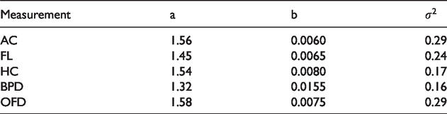
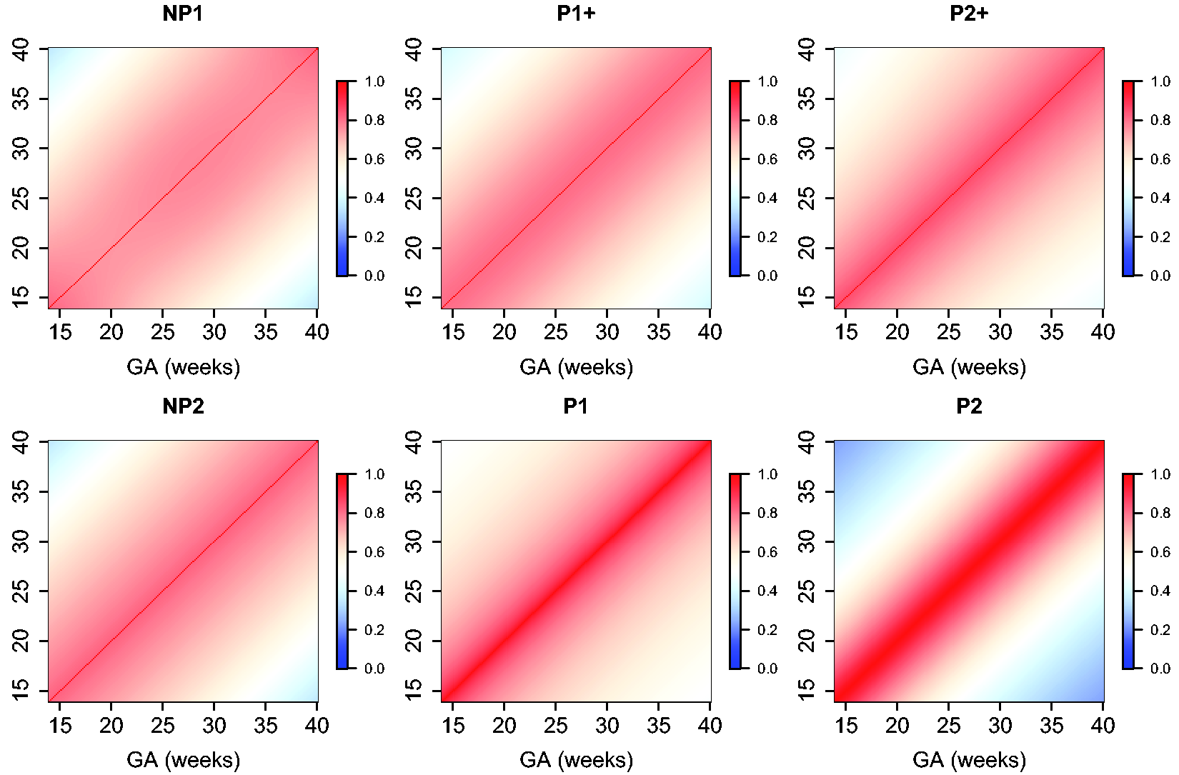
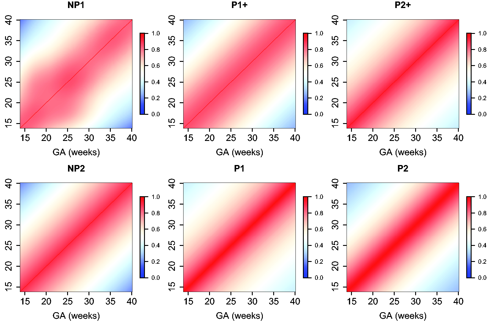
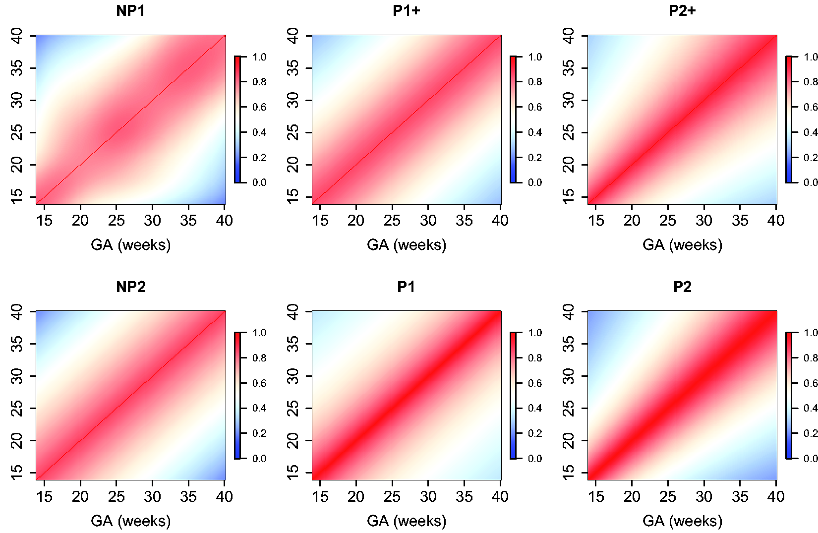
The estimated parameters for a P1+ model are summarized in Table 5. For illustration, we plot the fitted correlation surface on a grid of gestational age by weeks for AC in Figure 6. Correlation plots for FL, HC, BPD, and OFD are given in Figures 7 to 10.
Estimated parameters for P1+ correlation models.
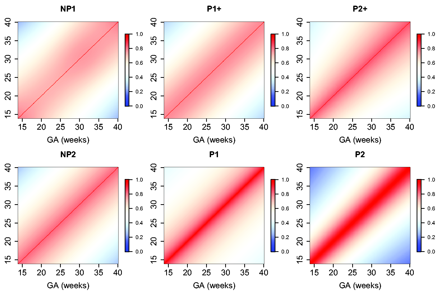
Temporal correlations of standardized AC with different correlation models.
Temporal correlations of standardized FL with different correlation models.
Temporal correlations of standardized HC with different correlation models.
Temporal correlations of standardized BPD with different correlation models.
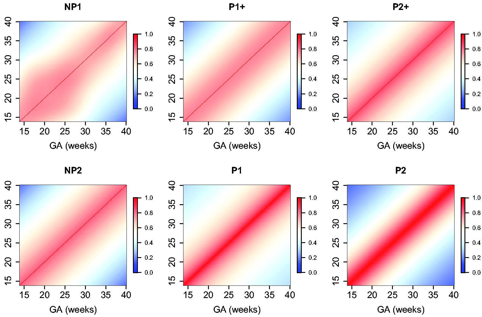
Temporal correlations of standardized OFD with different correlation models.
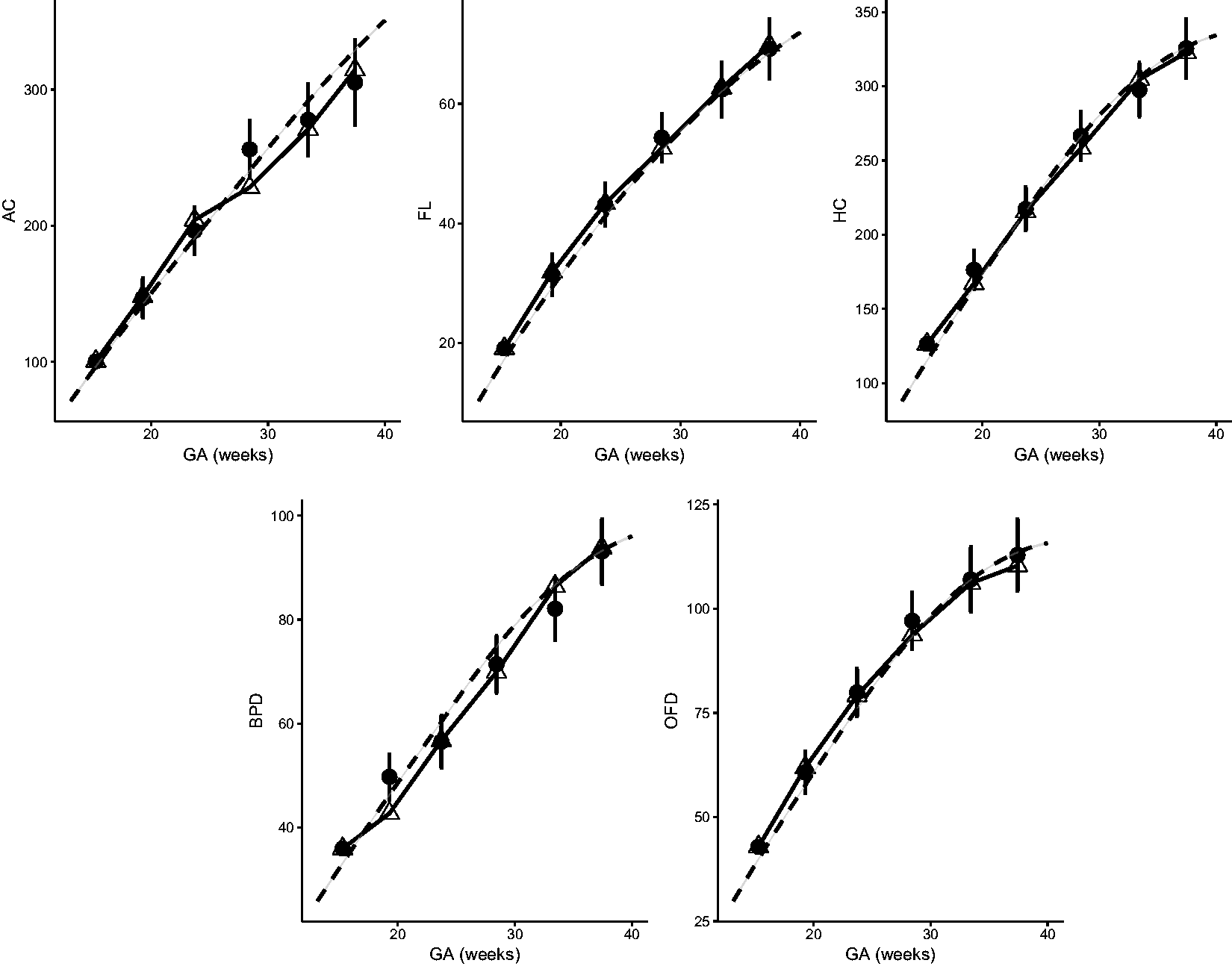
Observed growth trajectory (linked triangles) and predicted measurements (dots) given previous observations of a randomly selected fetus. Dashed line is the population mean.
5 Case study: dynamic growth velocity
We study the growth velocity of a randomly selected fetus using the fitted parametric correlation model, whose AC, FL, HC, BPD, and OFD are measured on six occasions between week 15 and week 38. The observed growth trajectories are shown as linked triangles in Figure 11. Based on each observed measurement at Tj, we also dynamically predict the measurement
For this fetus, selected as random, the growth is regular for FL and HC and can be predicted accurately. For AC, its measurements are higher (still normal) than predicted during the third visit, but much lower than expected during the fourth visit. This suggests that closer monitoring might be needed. The following visits indicate that the AC of the sampled fetus falls consistently below the population mean.
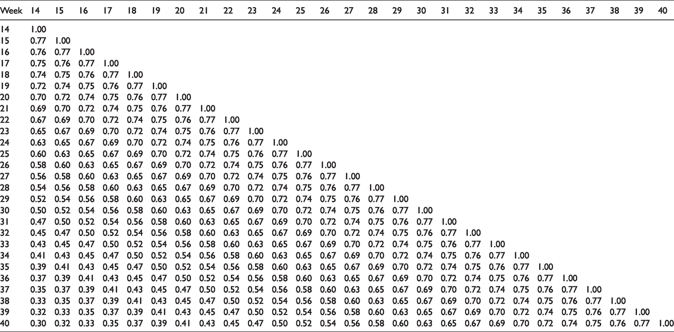
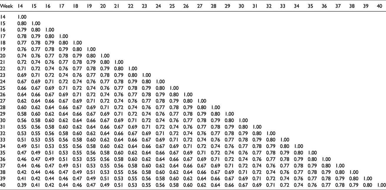
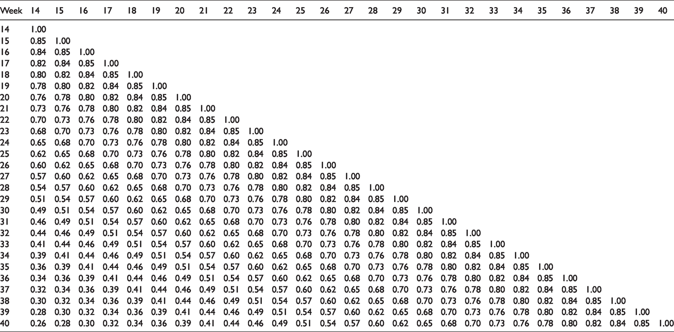
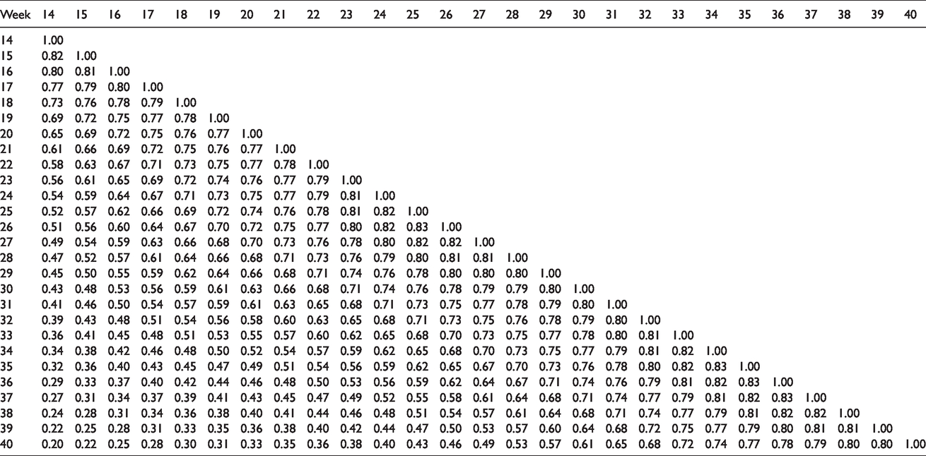
To facilitate the usage of the results in practice, a Shiny application is built along with this paper, where functionalities such as visualization, calculating correlation, prediction and cSDS are integrated for all the five fetal growth measurements (https://lxiao5.shinyapps.io/shinycalculator/). Correlation tables for fetal growth measurements are provided in Tables 6 to 10. The correlations are for weekly intervals, so the results are presented in the form of five 27 x 27 correlation matrices.
6 Discussion
We have modelled the correlation function of the fetal growth for transformed HC, BPD, OFD, AC, and FL. Its values are the correlations of two measurements of these five variables made at any time points between 14 and 40 weeks. The FGLS cohort remained healthy with adequate growth and motor development up to 2 years of age, hence making the characterization of the expected correlation of fetal size measurements ideal.9,11,12,15,28
The fit of the model for the correlations is adequate.
Correlation matrix for AC.
Correlation matrix for FL.
Correlation matrix for HC.
Correlation matrix for BPD.
Regression models such as in Ivanescu et al. 29 may also be used but in general are more difficult to deal with when the data are highly non-normal, as is the case for fetal metrics. The proposed two-stage approach is conceptually simpler, yields easy-to-interpret results, and achieves several aims. First, it gives a marginal standard chart that well handles non-normality of the measurements. Second, the correlation model combined with the marginal standard chart provides a parsimonious approach to prediction and inference at a future visit. Indeed, not only could we predict a future growth given the previous visits (one visit, two visits, etc.) along with a prediction interval, but also we could assess if the current growth is within normal bounds given the previous records.
Although velocity charts could be an important complement to attained size charts, 9 they are not often used clinically. For example, a clinician may be interested to know whether fetal HC at 20 weeks is a good predictor of that same fetuses HC at 30 weeks. From the correlation between 20 and 30 weeks, we can predict the value of fetal HC at 30 weeks based on its value at 20 weeks. Such prediction can identify fetuses that lag behind in growth.
A limitation of the study is paucity of data and small sample sizes for some pairs of gestational ages especially in early gestation (first trimester) and at term (40 weeks).
In summary, we provide formulae for correlation coefficients for fetal biometry using prospectively collected data in eight countries and diverse settings. They were collected using unified protocols, measurement procedures and standardization. A rigorous data quality process was in place throughout the study. INTERGROWTH-21st Project is the largest prospective study of fetal growth involving multiple measurements per fetus. The correlation coefficients for any pair of data between 14 and 40 weeks and consequently the calculation of a velocity Z-score provide a tool for monitoring fetal growth and development over time. To facilitate this, a web application (Shiny application for now) that calculates the expected correlation between any two time points in the interval 14 to 40 weeks for HC, AC, FL, BPD, and OFD will be made freely available on the INTERGROWTH-21st website where other applications for fetal, preterm, and newborn size are already available (https://intergrowth21.tghn.org/).
Our proposed two-stage approach can be able to accommodate simultaneous modelling of multiple fetal metrics by adapting our two-stage approach. The marginal standard charts can be estimated the same way as the first stage. Then we treat the transformed Z-scores as multiple measurements that are longitudinally observed and model the correlations across measurements and between different times. One option is a nonparametric multivariate functional data analysis. 30
Footnotes
Acknowledgement
We would like to thank the INTERGROWTH-21st Project team and participants who contributed data.
Declaration of conflicting interests
The author(s) declared no potential conflicts of interest with respect to the research, authorship, and/or publication of this article.
Funding
The author(s) disclosed receipt of the following financial support for the research, authorship, and/or publication of this article: This study was funded by the INTERGROWTH-21st grant 49038 from the Bill & Melinda Gates Foundation to the University of Oxford. LX was partially supported by Grant Number R01NS091307 from National Institute of Neurological Disorders and Stroke (NINDS) and Grant Number R56AG064803 from National Institute on Aging (NIA).