Optimal designs for asymmetric sigmoidal response curves in bioassays and immunoassays

Abstract

The 5-parameter logistic (5PL) model is frequently used to model and analyze responses from bioassays and immunoassays which can be skewed. Various types of optimal experimental designs for 2, 3 and 4-parameter logistic models have been reported but not for the more complicated 5PL model. We construct different types of optimal designs for studying various features of the 5PL model and show that commonly used designs in bioassays and immunoassays are generally inefficient for statistical inference. To facilitate use of such designs in practice, we create a user-friendly software package to generate various tailor-made optimal designs for the 5PL model and evaluate robustness properties of a design under a variation of criteria, model forms and misspecification in the nominal values of the model parameters.

1 Introduction

The 3-parameter logistic (3PL) and 4-parameter logistic (4PL) models are widely used to capture a symmetric sigmoidal relationship between the response and dose concentration. Recent studies show that asymmetrical response curves are often observed in various bioassays and immunoassays.^1–4 For such asymmetrical sigmoidal response curves, the 3PL and 4PL models are inappropriate. Gottschalk and Dunn ⁵ showed that the 5-parameter logistic (5PL) model is able to capture the asymmetric relationships adequately and produce more accurate inference for the assays compared to results using the 3PL or 4PL models.

Statistical inference for bioassays and immunoassays based on the 5PL model is not new. For example, Findlay and Dillard ⁶ applied the 5PL model to fit the data for ligand binding assays and Feng et al. ⁷ presented a Bayesian approach to fit the 5PL model using data from an enzyme-linked immunosorbent assay (ELISA). Dawn et al.^8,9 used a modified 5PL model (5PL-1P) to capture the asymmetry in mixture toxicity assessment and Cumberland ¹⁰ discussed the choice between the 4PL and 5PL models for estimation purposes; see also model fitting issues using biological data for these models in Davis et al. ¹¹ Another application of the 5PL model is Gottschalk and Dunn, ¹² who applied the model for measuring parallelism and relative potency in biological applications.

The design of a scientific study plays a crucial role in the accuracy of the inference that follows. Many of the above studies for the 5PL model used between 5 and 10 evenly spaced design points on the log scale with equal replication at each dose. This seems to be the current practice even though there is very little research in the literature to support such design choices. Manukyan and Rosenberger ¹³ appears to be the first who found locally D-optimal designs for the 5PL model when the response is binary.

The 3, 4 and 5PL models are frequently used to describe sigmoidal response curves and use of a wrong model can produce inaccurate or wrong inference. For example, optimal designs for the 3PL model cannot estimate all parameters in the 5PL model and an optimal design for the 5PL model can perform poorly when the 3PL or 4PL model holds. The implemented design should therefore provide good efficiencies when there are misspecifications in the nominal values, mean response assumptions and under a variation of criteria. Designs that provide relatively high efficiencies under model misspecifications are robust.

In practice, there are several objectives in the study and some are more important than others. This calls for a multiple-objective optimal design that can deliver user-specified efficiencies commensurate with the importance of each of the objectives. Such an optimal design is also appropriate when some parameters in the model are more interpretable than others. For instance, in the widely used two-parameter Michaelis-Menten model in the biological sciences, the Michaelis-Menten parameter is more interesting than the saturation parameter because it governs how fast the enzyme-substract kinetics reaction velocity is. It follows that the user should devote more resources to estimating the more interesting parameter or parameters so that they are more accurately estimated. Research to date shows a multiple-objective optimal design generally has overall higher efficiencies across all objectives than any of the single objective optimal designs can provide, see for example, Cook and Wong ¹⁴ and Hyun and Wong. ¹⁵ The former proposed a graphical approach to find dual-objective optimal designs using efficiency plots and, Hyun and Wong ¹⁵ gave a step-by-step approach to find 3-objective optimal designs for a nonlinear model. Of course, if the efficiencies sought under all the objectives are too high, a multiple-objective optimal design may not exist.

This paper has two aims. First, we focus on bioassays and immunoassays applications and find a variety of optimal designs for the 5PL model to accurately estimate (1) the model parameters in the model or (2) a target dose such as the EC₅₀ that results in having one half of test subject having the maximal expected response. Since model uncertainty is always an issue, we assess efficiencies of the optimal designs when the true model or the nominal values are misspecified. Additionally, we find robust D-optimal designs when the study has multiple objectives and the true model may be the 3PL, 4PL or 5PL model. Our second aim is to facilitate practitioners implement optimal designs and evaluate other designs for the 5PL model using an R package. Because the 5PL model is an extension of the 3PL and 4PL models, our functions can also readily find various optimal designs for the latter models.

Section 2 describes the response curve, and interprets the meaning of each parameter in the 5PL model and derivation of the Fisher information matrix. Section 3 presents several types of locally optimal designs for the 5PL model and a robust D-optimal design that performs well for the 3PL, 4PL, and 5PL models for estimating model parameters. In Section 4, we propose an algorithm with R functions to search for all the optimal designs in this paper. Section 5 studies sensitivities of the locally D-optimal design for the 5PL model when there are various misspecifications in the model assumptions. In Section 6, we recommend an efficient design and show it outperforms currently used designs in immunoassays and bioassays. Section 7 concludes with a summary of our work and future directions.

2 Background

Let X be the user-selected compact design space from which the design points are selected to observe the observations. Let Y _ij be the continuous response from the jth replicate at the ith concentration level $x_i\in X$ , where $j=1,\dots ,n_i,$ and $i=1,\dots ,K$ . Assume that we have resources to take a predetermined number of observations N so that $n_1+\dots +n_K=N$ . Given a design criterion, the design questions are the optimal number of design points to use, the optimal number of replicates and the location of each design point $x_i,i=1\dots ,x_K$ .

Let Θ be the vector of nominal values for the model parameters. Our statistical models have the form

$$Y_{\mathit{ij}}=f(x_i,\Theta )+{\varepsilon }_{\mathit{ij}},j=1,2,\dots ,n_i,i=1,2,\dots ,K,n_1+\dots +n_K=N$$

(1)

where $f(x_i,\Theta )$ is the mean response at x _i . The errors ∈ _ij s are independent and normally distributed with means 0 and unknown variance ${\sigma }^2$ .

We focus on approximate designs or large sample designs where we approximate each $n_i/N$ by its proportion. We denote such a design by $\xi =\{(x_i,w_i)\}1K$ where each $x_i\in X,w_i\in (0,1)$ and $w_1+\dots +w_K=1$ . In dose–response experiments, optimal design issues concern the total number of concentrations to be used (K), where these K concentration levels or design points $x_i,$ $i=1,2,\dots ,K$ are, and the proportions $w_i,i=1,\dots ,K$ of subjects to be allocated to each of these concentrations. Approximate designs can be studied under a unified framework and there are algorithms for finding many types of optimal designs. Formulas for such designs are available for many models and they facilitate studying properties of the optimal approximate designs. In addition, there are theoretical tools for verifying if an approximate design is optimal among all designs and the optimal approximate designs do not depend on the value of N by definition.

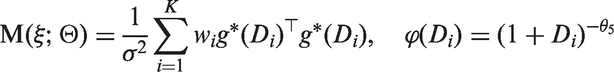
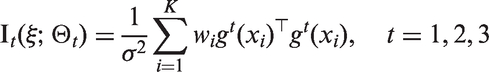
We measure the worth of a design by its Fisher information matrix. For the approximate design ξ, the normalized Fisher information matrix is

$$\text{I}(\xi ;\Theta )=\frac{1}{{\sigma }^2}\sum _{i=1}^K{w}_{i}g(x_i){\hspace{0.17em}}^{\top }g(x_i)$$

(2)

where $g(x)=(\begin{array}{cccc}\frac{\partial f(x,\Theta )}{\partial {\theta }_1},& \hfill \frac{\partial f(x,\Theta )}{\partial {\theta }_2},\hfill & \hfill \dots ,\hfill & \hfill \frac{\partial f(x,\Theta )}{\partial {\theta }_v}\hfill \end{array})$ and v is the number of model parameters. Since a ‘large’ information matrix is desirable for statistical inference, many optimality design criteria seek a design that makes this matrix as large as possible in different ways.

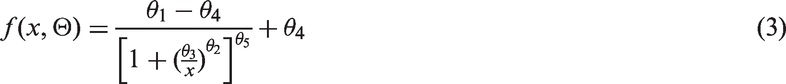
For the 5-parameter logistic (5PL) model, the mean response $f(x,\Theta )$ is

$$f(x,\Theta )=\frac{{\theta }_1-{\theta }_4}{[1+{(\frac{{\theta }_3}{x})}^{{\theta }_2}]{\theta }_5}+{\theta }_4$$

(3)

where θ₁ and θ₄ are the maximum and the minimum expected responses, respectively, θ₂ controls the stiffness of the response curve, θ₃ is the position of the transition region in concentration, and θ₅ is the asymmetric factor and takes a value greater than 0. The parameters θ₂ and θ₅ jointly control the slope of the response curve. Clearly, the 5PL model becomes the 4-parameter logistic (4PL) model when θ₅ takes the value of 1, and it becomes the 3-parameter logistic (3PL) model when θ₄ and θ₅ take the values of 0 and 1, respectively.

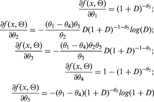
For the 5PL model, the vector g(x) has components given by

$$\begin{array}{c}\frac{\partial f(x,\Theta )}{\partial {\theta }_1}=(1+D)-{\theta }_5;\hfill \\ \frac{\partial f(x,\Theta )}{\partial {\theta }_2}=-\frac{({\theta }_1-{\theta }_4){\theta }_5}{{\theta }_2}D(1+D)-1-{\theta }_5\text{log}(D);\hfill \\ \frac{\partial f(x,\Theta )}{\partial {\theta }_3}=-\frac{({\theta }_1-{\theta }_4){\theta }_2{\theta }_5}{{\theta }_3}D(1+D)-1-{\theta }_5;\hfill \\ \frac{\partial f(x,\Theta )}{\partial {\theta }_4}=1-(1+D)-{\theta }_5;\hfill \\ \frac{\partial f(x,\Theta )}{\partial {\theta }_5}=-({\theta }_1-{\theta }_4)(1+D)-{\theta }_5\text{log}(1+D)\hfill \end{array}$$

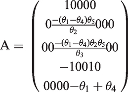
where $D=(\frac{{\theta }_3}{x}){\theta }_2$ . A direct calculation shows that the normalized Fisher information matrix (2) is $\text{I}(\xi ;\Theta )=A\text{M}(\xi ;\Theta )A^{\top }$ , where

$$\text{A}=\begin{array}{c}(\begin{array}{ccccc}1& \hfill 0\hfill & \hfill 0\hfill & \hfill 0\hfill & \hfill 0\hfill \\ 0& \hfill \frac{-({\theta }_1-{\theta }_4){\theta }_5}{{\theta }_2}\hfill & \hfill 0\hfill & \hfill 0\hfill & \hfill 0\hfill \\ 0& \hfill 0\hfill & \hfill \frac{-({\theta }_1-{\theta }_4){\theta }_2{\theta }_5}{{\theta }_3}\hfill & \hfill 0\hfill & \hfill 0\hfill \\ -1& \hfill 0\hfill & \hfill 0\hfill & \hfill 1\hfill & \hfill 0\hfill \\ 0& \hfill 0\hfill & \hfill 0\hfill & \hfill 0\hfill & \hfill -{\theta }_1+{\theta }_4\hfill \end{array})\end{array}$$

$$\text{M}(\xi ;\Theta )=\frac{1}{{\sigma }^2}\sum _{i=1}^K{w}_i{g}^{*}(D_i){\hspace{0.17em}}^{\top }{g}^{*}(D_i),\varphi (D_i)=(1+D_i)-{\theta }_5$$

and $g^{*}(D_i)=\varphi (D_i)(\begin{array}{ccccc}1,& \hfill \frac{D_i\text{log}(D_i)}{1+D_i},\hfill & \hfill \frac{D_i}{1+D_i},\hfill & \hfill \varphi {(D_i)}^{-1},\hfill & \hfill \text{log}(1+D_i)\hfill \end{array}).$ The matrix A does not contain any concentration level or weight and this implies that maximizing some function of $\text{M}(\xi ;\Theta )$ is equivalent to maximizing the same function in $\text{I}(\xi ;\Theta )$ . We observe that $\text{M}(\xi ;\Theta )$ contains only the three parameters θ₂, θ₃, and θ₅, and so any classical optimal design such as D-, A-, c-, or D _s -optimal design for model (3) does not depend on the parameters θ₁ and θ₄.

3 Optimal designs

The optimal design depends on the objective or objectives of the study. They can vary from estimating all or some model parameters to predicting mean response at a location in the design space or minimizing the sum of elements in the covariance matrix. Frequently, the criterion is formulated as a convex function of the information matrix so that we can use an equivalence theorem to check if the design is optimal among all designs. The equivalence theorem is derived from the directional derivative consideration and is unique for each convex functional; see design monographs, such as Fedorov ¹⁶ and Atkinson et al. ¹⁷ However, equivalence theorems all have a similar form as an inequality with 0 on the right-hand side of the inequality. The function on the left-hand side of the inequality is frequently called the sensitivity function in the literature.

The information matrix for a nonlinear model depends on the model parameters and so our optimal design depends on the unknown parameters. Such designs are termed locally optimal. ¹⁸ These optimal designs can be sensitive to the nominal values and so they must be selected carefully. However, they are the easiest to find and are important because they typically represent a first step to finding more complex designs. ¹⁹ Two approaches that do not require a set of single best guesses for the values of the parameters to find optimal designs are the Bayesian and minimax or maxmin approaches. The former requires a prior distribution for the parameters and the latter requires the user to specify a plausible region of possible values for all the parameters. Both methods generalize the concept of locally optimal designs and both Bayesian and minimax type of optimal designs are clearly much more difficult to find, theoretically or computationally, than locally optimal designs. For example, minimax optimal designs are found under a non-differentiable criterion and there are no effective algorithms for finding them for a general regression model. Chen et al. ²⁰ provide examples of minimax and standardized minimax optimal designs, including showing how locally optimal designs are first determined before a standardized minimax optimal design is found. Recent work on maximin optimal designs, which are equivalent to minimax optimal designs, and Bayesian optimal designs are Coffey ²¹ and McCallum and Bornkamp, ²² respectively, among others. For space consideration, these two approaches will not be further discussed here.

We now review several commonly used locally optimal designs in practice. In what follows, we use the terms locally optimal designs and optimal designs interchangeably when there is no room for confusion.

3.1 D-optimal designs for estimating Θ

D-optimal designs are the most appropriate when the interest in the study is to estimate the vector of model parameters Θ as accurately as possible. The D-optimal design ξ _D maximizes the determinant of the Fisher information matrix $\left|{\text{I}}_{(\xi ;\Theta )}\right|$ over all designs on X. Equivalently, for fixed Θ, we want a design that minimizes the convex function $-\text{log}\left|{\text{I}}_{(\xi ;\Theta )}\right|$ . The directional derivative of the D-optimality criterion leads to the sensitivity function: $d_D(x,\xi )=g(x){\text{I}}^{-1}(\xi ;\Theta )g(x){\hspace{0.17em}}^{\top }-5$ . The Equivalence Theorem states that design ξ _D is D-optimal for the 5PL model if and only if

$$d_D(x,{\xi }_D)\le 0$$

for all x in X with equality at the design points of ξ _D .

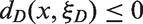
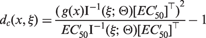
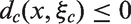
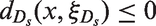
3.2 c-Optimal designs for estimating the EC₅₀

A c-optimal design is used to estimate a function of model parameters as accurately as possible by minimizing the asymptotic variance of its estimate. The EC₅₀ is the concentration producing a response that is half way between the expected maximum and minimum responses. A direct calculation shows

$$E{C}_{50}={\text{arg}}_x\{f(x,\Theta )=\frac{1}{2}({\theta }_1+{\theta }_4)\}={\theta }_3(\hspace{0.17em}2{\theta }_5^{-1}-1)-1/{\theta }_2$$

If ${\widehat{\mathit{EC}}}_{50}$ is the maximum likelihood estimate of EC₅₀, the c-optimal design for estimating the EC₅₀, ξ _c minimizes $\mathit{Var}({\widehat{\mathit{EC}}}_{50})=EC\text{'}{\hspace{0.17em}}_{50}{\text{I}}^{-1}(\xi ;\Theta )[EC\text{'}{\hspace{0.17em}}_{50}]{\hspace{0.17em}}^{\top },$ where $EC\text{'}{\hspace{0.17em}}_{50}$ is the derivative of the EC₅₀ with respect to Θ, i.e.

$$EC\text{'}{\hspace{0.17em}}_{50}=(\begin{array}{ccccc}0,& \hfill \frac{1}{{\theta }_2^2}E{C}_{50}\text{log}(\hspace{0.17em}2{\theta }_5^{-1}-1),\hfill & \hfill \frac{1}{{\theta }_3}E{C}_{50},\hfill & \hfill 0,\hfill & \hfill \frac{1}{{\theta }_2{\theta }_3^{{\theta }_2}{\theta }_5^2}\hspace{0.17em}2{\theta }_5^{-1}{\mathit{EC}}_{50}^{{\theta }_2+1}\text{log}(2)\hfill \end{array})$$

Consideration of the directional derivative of the c-optimality criterion leads to the sensitivity function

$$d_c(x,\xi )=\frac{{(g(x){\text{I}}^{-1}(\xi ;\Theta ){[EC\text{'}{\hspace{0.17em}}_{50}]}^{\top })}^2}{EC\text{'}{\hspace{0.17em}}_{50}{\text{I}}^{-1}(\xi ;\Theta ){[EC\text{'}{\hspace{0.17em}}_{50}]}^{\top }}-1$$

and the Equivalence Theorem states that design ξ _c is c-optimal for the 5PL model if and only if

$$d_c(x,{\xi }_c)\le 0$$

for all x in X with equality at the design points of ξ _c .

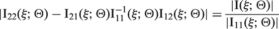
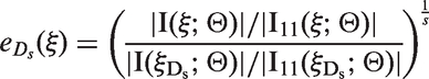
3.3 D_s-optimal designs for estimating the θ₅

A D _s -optimal design is used to estimate one or more model parameters. If one assumes the 5PL model, one may wish to estimate θ₅ accurately since the 5PL model becomes the 4PL model when ${\theta }_5=1$ . Clearly if there is a single parameter of interest, D _s -optimality reduces to c-optimality. When there are multiple parameters of interest, the D _s -optimal design minimizes the generalized variance of the estimated parameters. One proceeds by first partitioning the Fisher information matrix (2) suitably

$$\text{I}(\xi ;\Theta )=\frac{1}{{\sigma }^2}(\begin{array}{cc}{\text{I}}_{11}(\xi ;\Theta )& \hfill {\text{I}}_{12}(\xi ;\Theta )\hfill \\ {\text{I}}_{21}(\xi ;\Theta )& \hfill {\text{I}}_{22}(\xi ;\Theta )\hfill \end{array})$$

(4)

where ${\text{I}}_{\text{uv}}(\xi ;\Theta )=\sum _{i=1}^K{w}_i{g}_u(x_i){\hspace{0.17em}}^{\top }{g}_v(x_i),$ $u,v=1,2$ . For example, if estimating θ₅ in the 5PL model is the key objective, we let

$$g_1(x)=(\begin{array}{cccc}\frac{\partial f(x,\Theta )}{\partial {\theta }_1},& \hfill \frac{\partial f(x,\Theta )}{\partial {\theta }_2},\hfill & \hfill \frac{\partial f(x,\Theta )}{\partial {\theta }_3},\hfill & \hfill \frac{\partial f(x,\Theta )}{\partial {\theta }_4}\hfill \end{array})\text{\hspace{1em}and\hspace{1em}}{g}_2(x)=(\begin{array}{c}\frac{\partial f(x,\Theta )}{\partial {\theta }_5}\end{array})$$

It follows that the variance of the estimated θ₅ is proportional to

$${\text{I}}^{22}(\xi ;\Theta )=\{{\text{I}}_{22}(\xi ;\Theta )-{\text{I}}_{21}(\xi ;\Theta ){\text{I}}_{11}^{-1}(\xi ;\Theta ){\text{I}}_{12}(\xi ;\Theta )\}-1$$

and the D _s -optimal design ${\xi }_{D_s}$ maximizes the determinant

$$|{\text{I}}_{22}(\xi ;\Theta )-{\text{I}}_{21}(\xi ;\Theta ){\text{I}}_{11}^{-1}(\xi ;\Theta ){\text{I}}_{12}(\xi ;\Theta )|=\frac{|\text{I}(\xi ;\Theta )|}{|{\text{I}}_{11}(\xi ;\Theta )|}$$

In particular, the directional derivative of the D _s -optimality criterion for estimating a subset of s of the parameters leads to the sensitivity function

$$d_{D_s}(x,\xi )=\{g(x){\text{I}}^{-1}(\xi ;\Theta )g{(x)}^{\top }-g_1(x){\text{I}}_{11}^{-1}(\xi ;\Theta )g_1{(x)}^{\top }\}-s$$

In our case, since we have only one parameter of interest, we set s = 1. The Equivalence Theorem states that design ${\xi }_{D_s}$ is D _s -optimal if and only if

$$d_{D_s}(x,{\xi }_{D_s})\le 0$$

for all x in X with equality at the design points of ${\xi }_{D_s}$ .

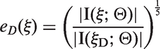
3.4 Design efficiency

We use design efficiency to compare the worth of a design relative to the optimum. This is a value between 0 and 1 and frequently it is simply the ratio of the optimal values of the criterion evaluated for the two designs or some simple function thereof. The interpretation of the efficiency of a design is that if its value is r, this design requires $100(1/r-1)\%$ more observations to do as well as the optimal design. For example, when $e_D(\xi )=0.5$ for a given design ξ, this design requires 200% more observations to provide the same D-optimality criterion value as the D-optimal design does and this tells that twice as many observations are required for the design to be as efficient as the D-optimal design. The performance of a design ξ for estimating Θ is given by its D-efficiency

$$e_D(\xi )=(\frac{|\text{I}(\xi ;\Theta )|}{|\text{I}({\xi }_{\text{D}};\Theta )|}{)}^{\frac{1}{5}}$$

Likewise, for estimating a given function of the model parameters, say EC₅₀ using design ξ, its c-efficiency is

$$e_c(\xi )=\frac{\mathit{EC}\text{'}{\hspace{0.17em}}_{50}{\text{I}}^{-1}({\xi }_{\text{c}};\Theta ){[\mathit{EC}\text{'}{\hspace{0.17em}}_{50}]}^{\top }}{EC\text{'}{\hspace{0.17em}}_{50}{\text{I}}^{-1}(\xi ;\Theta ){[\mathit{EC}\text{'}{\hspace{0.17em}}_{50}]}^{\top }}$$

where ξ _c is a EC₅₀-optimal design. Similarly, the D _s -efficiency of a design ξ for estimating s parameters in the model is

$$e_{D_s}(\xi )=(\frac{|\text{I}(\xi ;\Theta )|/|{\text{I}}_{11}(\xi ;\Theta )|}{|\text{I}({\xi }_{{\text{D}}_{\text{s}}};\Theta )|/|{\text{I}}_{11}({\xi }_{{\text{D}}_{\text{s}}};\Theta )|}{)}^{\frac{1}{s}}$$

In practice, we want the implemented design to have high efficiency under the user-specified criterion and ideally a design with relatively high efficiencies across criteria and under a variety of model violations.

3.5 A robust D-optimal design to model misspecification

Locally optimal designs can be sensitive to misspecifications in a nonlinear model, including nominal values which we need to construct a locally optimal design. Here we propose a robust locally D-optimal design that has relatively high efficiencies for estimating parameters in the 3PL, 4PL and 5PL models.

Let ${\Theta }_1,{\Theta }_2,{\Theta }_3$ be the vectors of nominal values for the model parameters in the 3PL, 4PL, 5PL models, respectively, and let $g^1(x),g^2(x),g^3(x)$ be the gradients of the mean functions for the three models respectively. The normalized Fisher information matrices for each of the model is

$${\text{I}}_t(\xi ;{\Theta }_t)=\frac{1}{{\sigma }^2}\sum _{i=1}^K{w}_i{g}^t(x_i){\hspace{0.17em}}^{\top }{g}^t(x_i),t=1,2,3$$

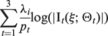
Following Cook and Wong ¹⁴ and Atkinson et al., ¹⁷ we use a compound design criterion to construct an efficient design to estimate model parameters accurately regardless which one of the three models holds. Given nominal values ${\Theta }_1,{\Theta }_2$ and ${\Theta }_3$ for the 3PL, 4PL and 5PL model, respectively, the sought locally optimal design maximizes a weighted average of the three D-optimality criteria for the three models, i.e.

$$\sum _{t=1}^3\frac{{\lambda }_i}{p_t}\text{log}(|{\text{I}}_t(\xi ;{\Theta }_t)|)$$

Here, p _t is the number of model parameters in the tth model and λ _t is a user-selected prior probability that the tth model holds with $\sum _{t=1}^3{\lambda }_t=1$ . By taking directional derivative of the above criterion, one can show the sensitivity function is

$$d_{\mathit{RoD}}(x,\xi )=\{\sum _{t=1}^3\frac{{\lambda }_t}{p_t}{d}_t(x,\xi )\}-1$$

(6)

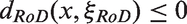
where $d_t(x,\xi )=g^t(x){\text{I}}_t^{-1}(\xi ;{\Theta }_t)g^t(x){\hspace{0.17em}}^{\top }$ . By the Equivalence Theorem, the design ξ _RoD is robust D-optimal design if and only if

$$d_{\mathit{RoD}}(x,{\xi }_{\mathit{RoD}})\le 0$$

for all x in X with equality at the design points of the design ξ _RoD .

4 An algorithm and R-package

Yang et al. ²³ introduced an efficient algorithm to search several types of optimal designs for nonlinear models and showed that it outperforms other well-known standard design algorithms. Hyun et al. ²⁴ modified their algorithm to search the optimal designs more efficiently and this modified algorithm is used to search all the optimal designs in this paper. Given a differentiable criterion Ψ, we first compute the first and the second derivatives of the optimality criterion with respect to the weights, $\frac{\partial \Psi }{\partial w_i}$ and $\frac{\partial {\hspace{0.17em}}^2\Psi }{\partial w_i{w}_j}$ . The algorithm selects good initial design points via the Fedorov's algorithm, ¹⁶ and at each iteration it selects the point that maximizes the sensitivity function $d(x,\xi )$ and adds it to the support of the current design. The optimal weights for the selected design points are then obtained by the Newton Raphson's method using $\frac{\partial \Psi }{\partial w_i}$ and $\frac{\partial {\hspace{0.17em}}^2\Psi }{\partial w_i{w}_j}$ . Upon convergence, the optimality of the design is verified by a General Equivalence Theorem for its optimality. ²⁵ To facilitate practitioners use our optimal designs, we have developed an R package Opt5PL based on this algorithm to search for all optimal designs in this paper and the package is available at the Comprehensive R Archive Network (https://CRAN.R-project.org/package=Opt5PL). The supplementary material for this paper contains illustrative examples showing how to use the package to obtain several optimal designs and their efficiencies reported in this paper.

The R package contains several functions (ROPT, EDpOPT, DsOPT, Deff, EDpeff, Dseff) useful for finding and evaluating optimal designs for the 5PL models, including functions for studying optimal designs for the 3PL or 4PL models. We describe a few here:

The ROPT function generates the robust D-optimal design when there is uncertainty among the 3PL, 4PL, and 5PL models. The function produces the D-optimal design for each model and the ROPT function maximizes the compound optimality criterion (5) and verifies the optimality of the generated design using an General Equivalence Theorem by producing a graphical plot of the sensitivity function (6).

We recall EC _p is the concentration level that achieves the $100p\%$ of the difference between the maximum and the minimum responses and the EDpOPT function finds the c-optimal design to estimate EC _p . When p = 0.5, this function finds the c-optimal design for estimating EC₅₀ in the 5PL model. Another function is the DsOPT function for finding the D _s -optimal design for estimating θ₅ in the 5PL model. Both functions verify optimality of the generated designs using an approrpiate General Equivalence Theorem.

Given a user-supplied design, the Deff, EDpeff, Dseff functions compute, respectively, its D-efficiency for estimating Θ, c-efficiency for estimating the EC _p , and D _s -efficiency for estimating θ₅ in the 5PL model. The function Deff can also be used to compute D-efficiencies of any design in the 3PL and 4PL models. Together, these functions generate different types of optimal designs for the 5PL model and evaluate their performances under various misspecifications in the model assumptions.

5 Robustness of the D-optimal design for the 5PL model

5.1 Robustness to the model parameter values and to the 4PL model

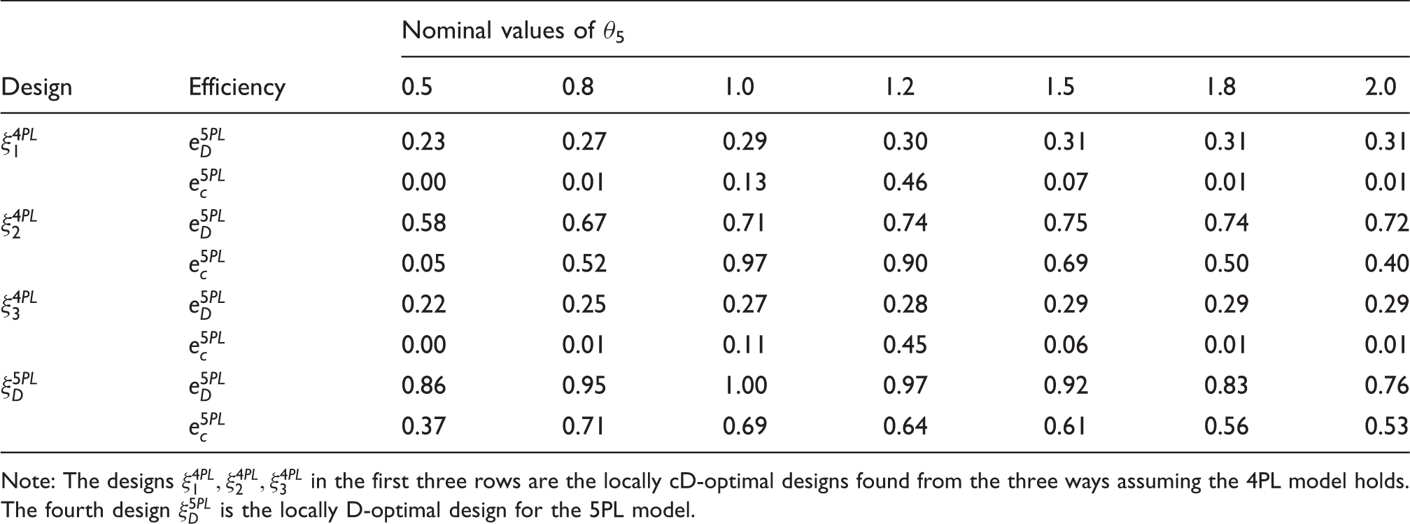
The 5PL model captures asymmetric levels of the response curve and so is a more flexible than the 3PL or 4PL model. Are optimal designs for the 5PL model robust to misspecification in nominal values or when the true model is the 4PL model? We provide some insights for the robustness properties for locally D-optimal designs for the 5PL model and also compare its performance with cD-optimal designs that combine c- and D-optimality in different ways to meet user-specified efficiencies for estimating both model parameters and EC₅₀. These cD-optimal designs were proposed by Holland ²⁶ and shown to perform well under the 4PL model for fitting symmetrical sigmoidal response curves only. Specifically, we consider the three types of cD-optimal designs shown in 2, 3b, and 4b in Table 1 of Holand-Latz's paper ²⁶ and denote them by ${\xi }_i^{4\mathit{PL}}$ , i = 1, 2, 3. They are, respectively, obtained by (i) maximizing a weighted geometric average of the c- and D- criteria, (ii) a two stage procedure using the idea of design augmentation in Padmanabhan, ²⁷ and (iii) maximizing a weighted geometric average of the c- and D- criteria subject to a user-specified constraint. In what is to follow, we check their performance compared to the D-optimal design for the 5PL model ${\xi }_D^{5\mathit{PL}}$ and evaluate the robustness of the four designs to misspecified parameter values and whether the true model is the 4PL or 5PL model.

Table 1.

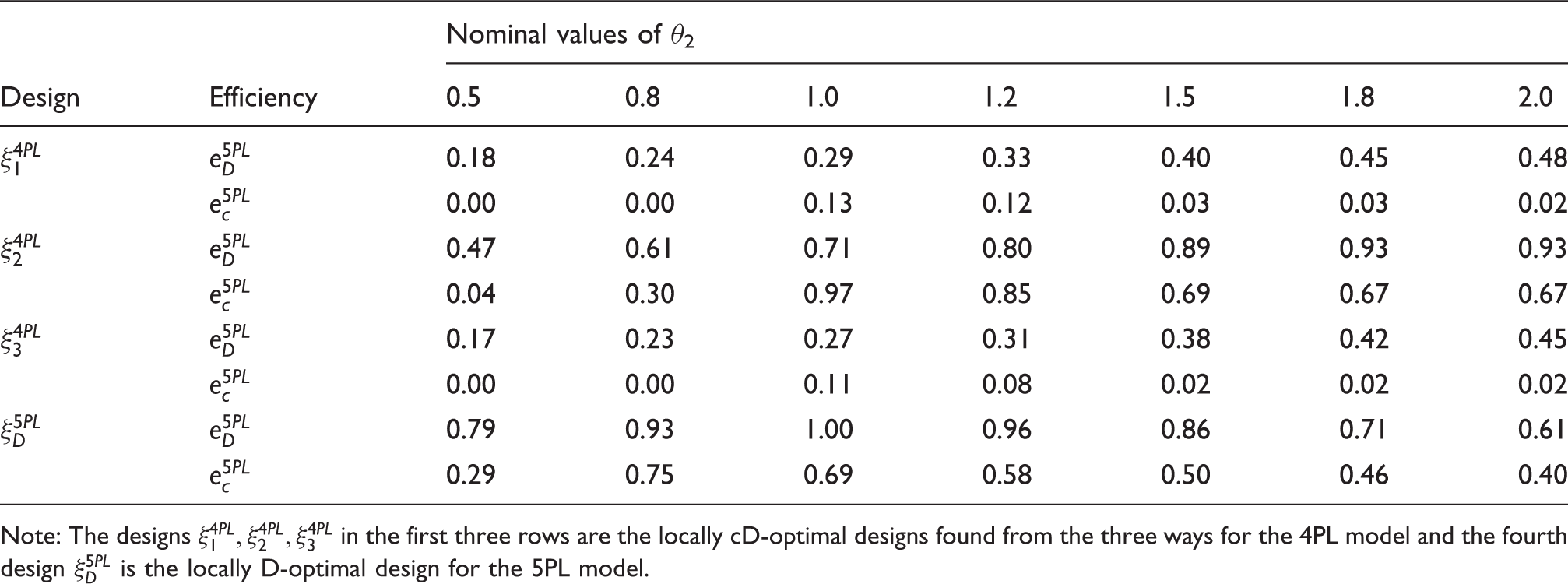
D-efficiencies, $e_D^{5\mathit{PL}}$ , and c-efficiencies, $e_c^{5\mathit{PL}}$ , of four designs under the 5PL model with various values of θ₅.

		Nominal values of θ5
Design	Efficiency	0.5	0.8	1.0	1.2	1.5	1.8	2.0
${\xi }_1^{4\mathit{PL}}$	$e_D^{5\mathit{PL}}$	0.23	0.27	0.29	0.30	0.31	0.31	0.31
	$e_c^{5\mathit{PL}}$	0.00	0.01	0.13	0.46	0.07	0.01	0.01
${\xi }_2^{4\mathit{PL}}$	$e_D^{5\mathit{PL}}$	0.58	0.67	0.71	0.74	0.75	0.74	0.72
	$e_c^{5\mathit{PL}}$	0.05	0.52	0.97	0.90	0.69	0.50	0.40
${\xi }_3^{4\mathit{PL}}$	$e_D^{5\mathit{PL}}$	0.22	0.25	0.27	0.28	0.29	0.29	0.29
	$e_c^{5\mathit{PL}}$	0.00	0.01	0.11	0.45	0.06	0.01	0.01
${\xi }_D^{5\mathit{PL}}$	$e_D^{5\mathit{PL}}$	0.86	0.95	1.00	0.97	0.92	0.83	0.76
	$e_c^{5\mathit{PL}}$	0.37	0.71	0.69	0.64	0.61	0.56	0.53

Note: The designs ${\xi }_1^{4\mathit{PL}},{\xi }_2^{4\mathit{PL}},{\xi }_3^{4\mathit{PL}}$ in the first three rows are the locally cD-optimal designs found from the three ways assuming the 4PL model holds. The fourth design ${\xi }_D^{5\mathit{PL}}$ is the locally D-optimal design for the 5PL model.

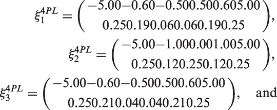
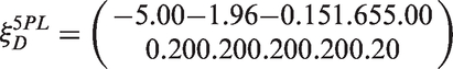
We use the same setup in Holland ²⁶ and the vector of nominal values for the 4PL model is ${\Theta }_2=({\theta }_1,{\theta }_2,{\theta }_3,{\theta }_4)=(1,1,1,0)$ and the log concentration range is between −5 and 5. For the same concentration range, the vector of nominal values for the 5PL model parameters is ${\Theta }_3=({\theta }_1,{\theta }_2,{\theta }_3,{\theta }_4,{\theta }_5)=(1,1,1,0,1)$ . We denote the three cD-optimal designs for the 4Pl model and the D-optimal design for the 5PL model, respectively, by ${\xi }_1^{4\mathit{PL}},{\xi }_2^{4\mathit{PL}},{\xi }_3^{4\mathit{PL}}$ , and ${\xi }_D^{5\mathit{PL}}$ and they are given by

$$\begin{array}{c}{\xi }_1^{4\mathit{PL}}=(\begin{array}{cccccc}-5.00& \hfill -0.60\hfill & \hfill -0.50\hfill & \hfill 0.50\hfill & \hfill 0.60\hfill & \hfill 5.00\hfill \\ 0.25& \hfill 0.19\hfill & \hfill 0.06\hfill & \hfill 0.06\hfill & \hfill 0.19\hfill & \hfill 0.25\hfill \end{array}),\hfill \\ {\xi }_2^{4\mathit{PL}}=(\begin{array}{ccccc}-5.00& \hfill -1.00\hfill & \hfill 0.00\hfill & \hfill 1.00\hfill & \hfill 5.00\hfill \\ 0.25& \hfill 0.12\hfill & \hfill 0.25\hfill & \hfill 0.12\hfill & \hfill 0.25\hfill \end{array}),\hfill \\ {\xi }_3^{4\mathit{PL}}=(\begin{array}{cccccc}-5.00& \hfill -0.60\hfill & \hfill -0.50\hfill & \hfill 0.50\hfill & \hfill 0.60\hfill & \hfill 5.00\hfill \\ 0.25& \hfill 0.21\hfill & \hfill 0.04\hfill & \hfill 0.04\hfill & \hfill 0.21\hfill & \hfill 0.25\hfill \end{array}),\text{\hspace{1em}and\hspace{1em}}\hfill \end{array}$$

$${\xi }_D^{5\mathit{PL}}=(\begin{array}{ccccc}-5.00& \hfill -1.96\hfill & \hfill -0.15\hfill & \hfill 1.65\hfill & \hfill 5.00\hfill \\ 0.20& \hfill 0.20\hfill & \hfill 0.20\hfill & \hfill 0.20\hfill & \hfill 0.20\hfill \end{array})$$

Tables 1 to 3 display D-efficiencies, $e_D^{5\mathit{PL}}$ , of the four designs ${\xi }_1^{4\mathit{PL}},{\xi }_2^{4\mathit{PL}},{\xi }_3^{4\mathit{PL}}$ , and ${\xi }_D^{5\mathit{PL}}$ for estimating the model parameters and their c-efficiencies, $e_c^{5\mathit{PL}}$ , for estimating the EC₅₀ when the 5PL model holds and one of the three parameters ${\theta }_5,{\theta }_2$ and θ₃ is misspecified, respectively. These cD-optimal designs have more than four design points and it is appropriate to ascertain whether they remain efficient for estimating all the parameters or EC₅₀ when the 5PL model holds. We note at the end of Section 2 that the design construction does not depend on the parameters θ₁ and θ₄ and so we do not investigate the drop in the design efficiencies when their nominal values are misspecified. In these and all tables to follow, zero efficiencies mean actual efficiencies are smaller than 0.01.

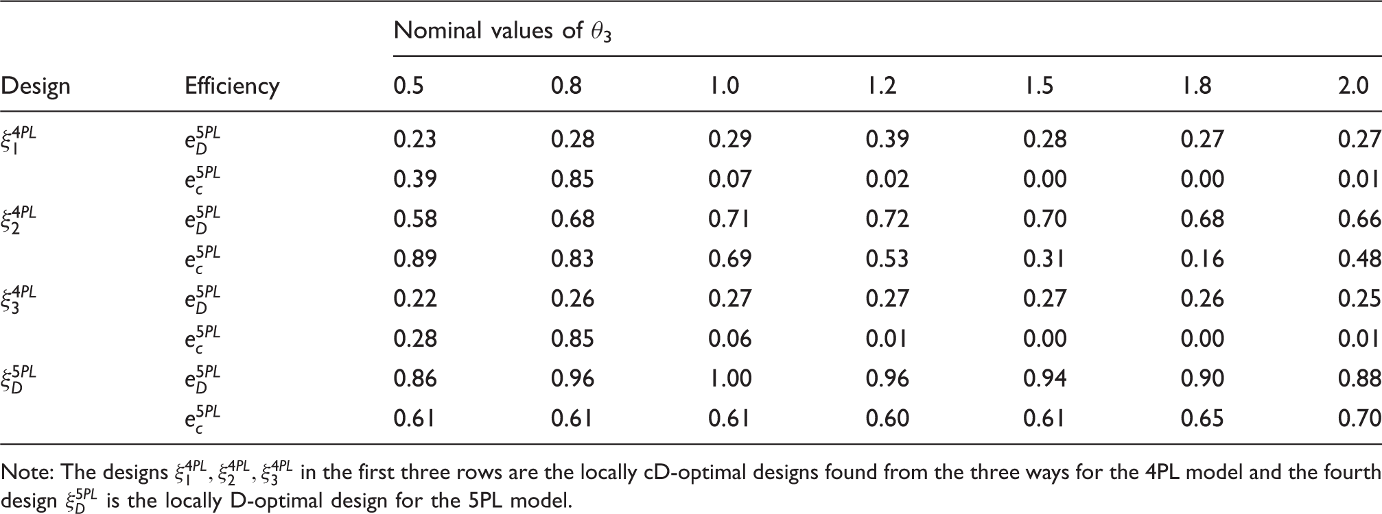
It is clear from Tables 1 to 3 that the three cD-optimal designs for the 4PL model do not perform well under the 5PL models when the values of θ₂, θ₃ or θ₅ are misspecified. The design ${\xi }_2^{4\mathit{PL}}$ performs better than the other two cD-optimal designs but the overall efficiencies for the three cD-optimal designs for either estimating parameters or for EC₅₀ are poor compared with those from ${\xi }_D^{5\mathit{PL}}$ , even in the case when ${\theta }_5=1$ when the two models coincide. There are two interesting exceptions: (i) Table 2 shows both D- and c-efficiencies of the design ${\xi }_2^{4\mathit{PL}}$ begin to outperform those from ${\xi }_D^{5\mathit{PL}}$ when the parameters are misspecified and larger than the true value, and (ii) Table 3 shows the c-efficiencies of the design ${\xi }_2^{4\mathit{PL}}$ outperform ${\xi }_D^{5\mathit{PL}}$ when the nominal value of θ₃ is misspecified and smaller than the true value. This reinforces the importance of considering the 5PL model to construct optimal designs and shows how the designs obtained from the 4PL model perform inefficiently when they are used for the 5PL model. In contrast, the D-optimal design ${\xi }_D^{5\mathit{PL}}$ works well for estimating the model parameters for the different values of θ₂, θ₃, and θ₅. The c-efficiencies of ${\xi }_D^{5\mathit{PL}}$ are lower than the D-efficiencies but mostly they are higher than ones for obtained from the cD-optimal designs. Additionally, Table 3 shows that the D- and c-efficiencies of the D-optimal design ${\xi }_D^{5\mathit{PL}}$ are much more consistent for different values of θ₃ when they are compared to the changes for different values of θ₂ and θ₅ in Tables 1 and 2. This tells that the D-optimal design for the 5PL model is more resistant to changes in the values of θ₃ than the changes in θ₂ and θ₅.

Table 2.

D-efficiencies $e_D^{5\mathit{PL}}$ and c-efficiencies $e_c^{5\mathit{PL}}$ of the locally optimal designs in column 1 when they are used for the 5PL model with various nominal values of θ₂.

		Nominal values of θ2
Design	Efficiency	0.5	0.8	1.0	1.2	1.5	1.8	2.0
${\xi }_1^{4\mathit{PL}}$	$e_D^{5\mathit{PL}}$	0.18	0.24	0.29	0.33	0.40	0.45	0.48
	$e_c^{5\mathit{PL}}$	0.00	0.00	0.13	0.12	0.03	0.03	0.02
${\xi }_2^{4\mathit{PL}}$	$e_D^{5\mathit{PL}}$	0.47	0.61	0.71	0.80	0.89	0.93	0.93
	$e_c^{5\mathit{PL}}$	0.04	0.30	0.97	0.85	0.69	0.67	0.67
${\xi }_3^{4\mathit{PL}}$	$e_D^{5\mathit{PL}}$	0.17	0.23	0.27	0.31	0.38	0.42	0.45
	$e_c^{5\mathit{PL}}$	0.00	0.00	0.11	0.08	0.02	0.02	0.02
${\xi }_D^{5\mathit{PL}}$	$e_D^{5\mathit{PL}}$	0.79	0.93	1.00	0.96	0.86	0.71	0.61
	$e_c^{5\mathit{PL}}$	0.29	0.75	0.69	0.58	0.50	0.46	0.40

Note: The designs ${\xi }_1^{4\mathit{PL}},{\xi }_2^{4\mathit{PL}},{\xi }_3^{4\mathit{PL}}$ in the first three rows are the locally cD-optimal designs found from the three ways for the 4PL model and the fourth design ${\xi }_D^{5\mathit{PL}}$ is the locally D-optimal design for the 5PL model.

Table 3.

D-efficiencies $e_D^{5\mathit{PL}}$ and c-efficiencies $e_c^{5\mathit{PL}}$ of the locally optimal designs in column 1 when they are used for the 5PL model with various nominal values of θ₃.

		Nominal values of θ3
Design	Efficiency	0.5	0.8	1.0	1.2	1.5	1.8	2.0
${\xi }_1^{4\mathit{PL}}$	$e_D^{5\mathit{PL}}$	0.23	0.28	0.29	0.39	0.28	0.27	0.27
	$e_c^{5\mathit{PL}}$	0.39	0.85	0.07	0.02	0.00	0.00	0.01
${\xi }_2^{4\mathit{PL}}$	$e_D^{5\mathit{PL}}$	0.58	0.68	0.71	0.72	0.70	0.68	0.66
	$e_c^{5\mathit{PL}}$	0.89	0.83	0.69	0.53	0.31	0.16	0.48
${\xi }_3^{4\mathit{PL}}$	$e_D^{5\mathit{PL}}$	0.22	0.26	0.27	0.27	0.27	0.26	0.25
	$e_c^{5\mathit{PL}}$	0.28	0.85	0.06	0.01	0.00	0.00	0.01
${\xi }_D^{5\mathit{PL}}$	$e_D^{5\mathit{PL}}$	0.86	0.96	1.00	0.96	0.94	0.90	0.88
	$e_c^{5\mathit{PL}}$	0.61	0.61	0.61	0.60	0.61	0.65	0.70

Note: The designs ${\xi }_1^{4\mathit{PL}},{\xi }_2^{4\mathit{PL}},{\xi }_3^{4\mathit{PL}}$ in the first three rows are the locally cD-optimal designs found from the three ways for the 4PL model and the fourth design ${\xi }_D^{5\mathit{PL}}$ is the locally D-optimal design for the 5PL model.

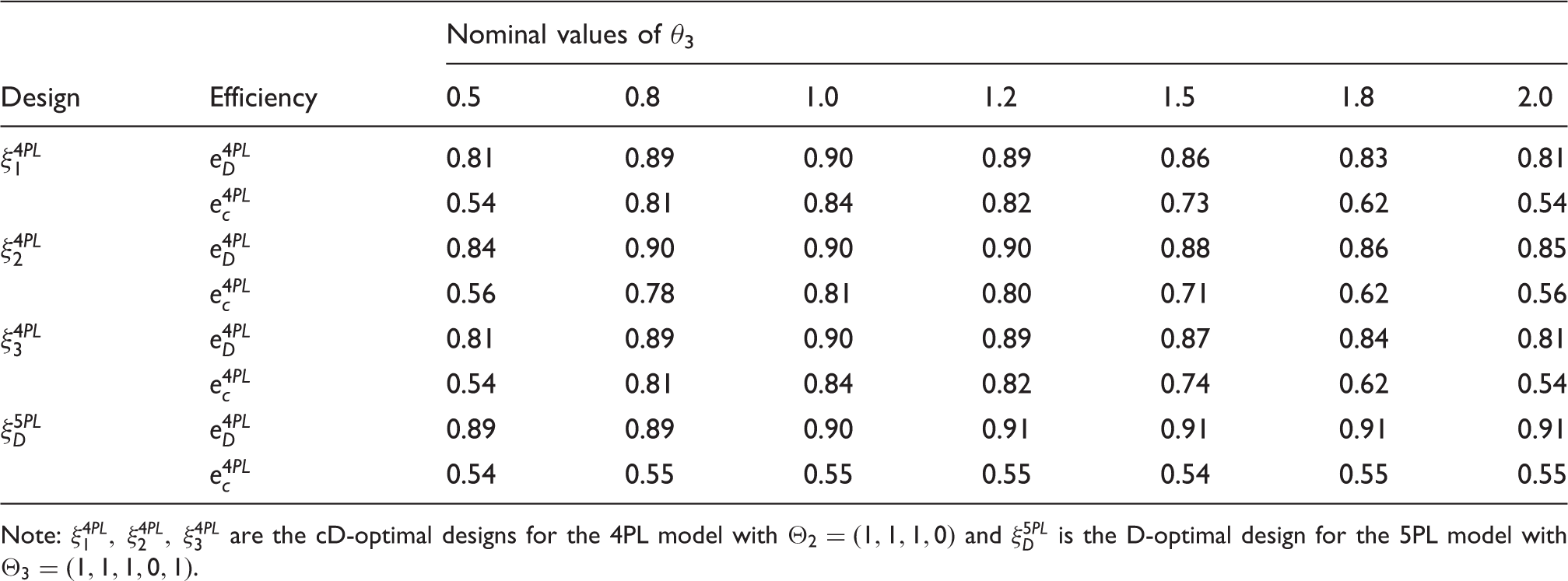
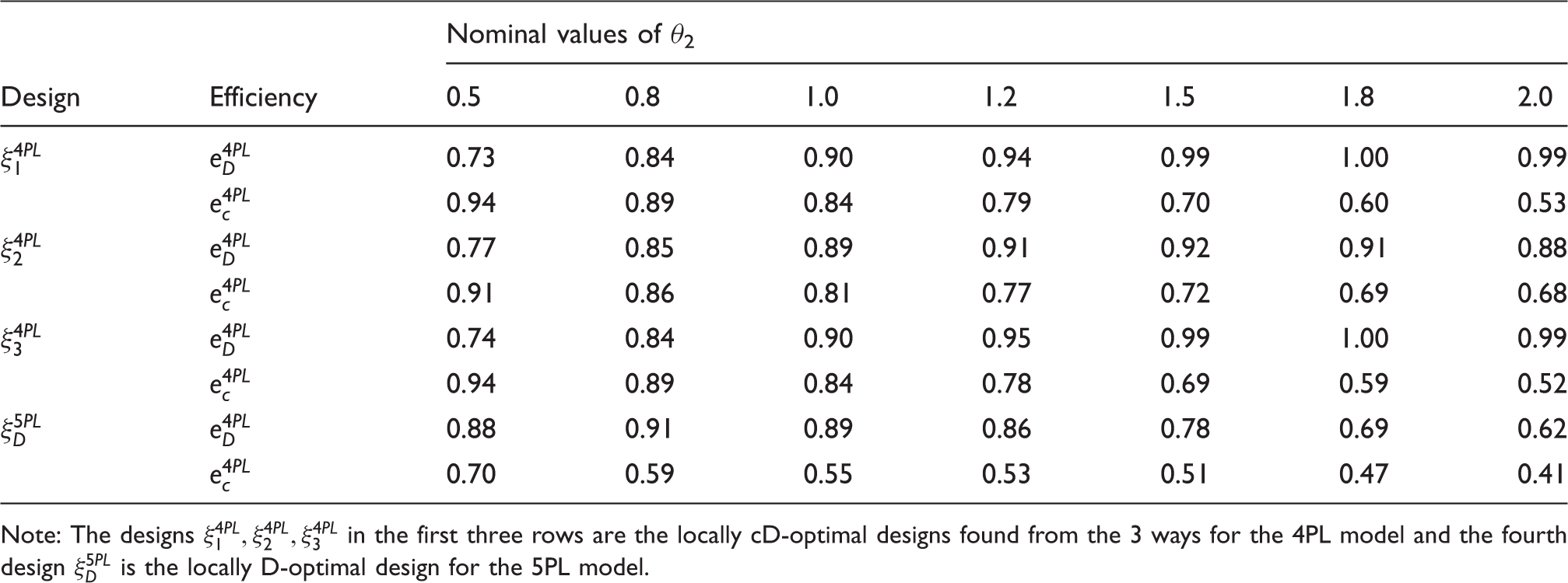
Tables 4 and 5 assume the 4PL model holds and compare D-efficiencies, $e_D^{4\mathit{PL}}$ , and c-efficiencies, $e_c^{4\mathit{PL}}$ of the four designs when one of the two parameters θ₃ and θ₂ is misspecified. Under the 4PL model, θ₃ represents the EC₅₀ and θ₂ represents the slope at the EC₅₀. The D-optimal design ${\xi }_D^{5\mathit{PL}}$ for the 5PL model performs well for the 4PL model when θ₃ is misspecified. However, their c-efficiencies are consistently smaller than those from the three cD-optimal designs, except when ${\theta }_3=0.5$ or 2.0. Table 5 shows a similar pattern with the three cD-optimal designs having higher c-efficiencies than those from the design ${\xi }_D^{5\mathit{PL}}$ when the 4PL model holds. Interestingly, Table 5 also shows that the design ${\xi }_D^{5\mathit{PL}}$ provides competitive D-efficiencies with those from cD-optimal designs but begins to loose ground when θ₂ is misspecified with a value larger than the true value assumed to be unity. The design ${\xi }_D^{5\mathit{PL}}$ does not take into account c-optimality criterion for estimating the EC₅₀ and so it is unsurprising that it has smaller c-efficiencies than its D-efficiencies for both the 4PL and the 5PL model, and also the same is true when compared with the cD-optimal designs that incorporate c-optimality.

Table 4.

D- and c-efficiencies, $e_D^{4\mathit{PL}}$ and $e_c^{4\mathit{PL}}$ of the four designs under the 4PL model with various values of θ₃.

		Nominal values of θ3
Design	Efficiency	0.5	0.8	1.0	1.2	1.5	1.8	2.0
${\xi }_1^{4\mathit{PL}}$	$e_D^{4\mathit{PL}}$	0.81	0.89	0.90	0.89	0.86	0.83	0.81
	$e_c^{4\mathit{PL}}$	0.54	0.81	0.84	0.82	0.73	0.62	0.54
${\xi }_2^{4\mathit{PL}}$	$e_D^{4\mathit{PL}}$	0.84	0.90	0.90	0.90	0.88	0.86	0.85
	$e_c^{4\mathit{PL}}$	0.56	0.78	0.81	0.80	0.71	0.62	0.56
${\xi }_3^{4\mathit{PL}}$	$e_D^{4\mathit{PL}}$	0.81	0.89	0.90	0.89	0.87	0.84	0.81
	$e_c^{4\mathit{PL}}$	0.54	0.81	0.84	0.82	0.74	0.62	0.54
${\xi }_D^{5\mathit{PL}}$	$e_D^{4\mathit{PL}}$	0.89	0.89	0.90	0.91	0.91	0.91	0.91
	$e_c^{4\mathit{PL}}$	0.54	0.55	0.55	0.55	0.54	0.55	0.55

Note: ${\xi }_1^{4\mathit{PL}},{\xi }_2^{4\mathit{PL}},{\xi }_3^{4\mathit{PL}}$ are the cD-optimal designs for the 4PL model with ${\Theta }_2=(1,1,1,0)$ and ${\xi }_D^{5\mathit{PL}}$ is the D-optimal design for the 5PL model with ${\Theta }_3=(1,1,1,0,1)$ .

Table 5.

D-efficiencies $e_D^{4\mathit{PL}}$ and c-efficiencies $e_c^{4\mathit{PL}}$ of locally optimal designs in column 1 when they are used for the 4PL model with various nominal values of the slope parameter θ₂.

		Nominal values of θ2
Design	Efficiency	0.5	0.8	1.0	1.2	1.5	1.8	2.0
${\xi }_1^{4\mathit{PL}}$	$e_D^{4\mathit{PL}}$	0.73	0.84	0.90	0.94	0.99	1.00	0.99
	$e_c^{4\mathit{PL}}$	0.94	0.89	0.84	0.79	0.70	0.60	0.53
${\xi }_2^{4\mathit{PL}}$	$e_D^{4\mathit{PL}}$	0.77	0.85	0.89	0.91	0.92	0.91	0.88
	$e_c^{4\mathit{PL}}$	0.91	0.86	0.81	0.77	0.72	0.69	0.68
${\xi }_3^{4\mathit{PL}}$	$e_D^{4\mathit{PL}}$	0.74	0.84	0.90	0.95	0.99	1.00	0.99
	$e_c^{4\mathit{PL}}$	0.94	0.89	0.84	0.78	0.69	0.59	0.52
${\xi }_D^{5\mathit{PL}}$	$e_D^{4\mathit{PL}}$	0.88	0.91	0.89	0.86	0.78	0.69	0.62
	$e_c^{4\mathit{PL}}$	0.70	0.59	0.55	0.53	0.51	0.47	0.41

Note: The designs ${\xi }_1^{4\mathit{PL}},{\xi }_2^{4\mathit{PL}},{\xi }_3^{4\mathit{PL}}$ in the first three rows are the locally cD-optimal designs found from the 3 ways for the 4PL model and the fourth design ${\xi }_D^{5\mathit{PL}}$ is the locally D-optimal design for the 5PL model.

6 Applications

In this section, we apply the R package Opt5PL to find locally D-optimal designs ξ _D , locally c-optimal designs ξ _c , and locally D _s -optimal designs ${\xi }_{D_s}$ for two bioassay studies and use them to evaluate efficiencies of the implemented designs. Both studies assume the 5PL model or a slightly modified version of it and come with nominal values. To study robustness properties of the various designs to misspecification in the nominal values of the model parameters, we consider six vectors of possible nominal values for the five model parameters and denote them by ${\Theta }_{31}-{\Theta }_{36}$ in Table 6. More details about how we arrived at the six different sets of nominal values for the parameters are given in section 6.1.

Table 6.

The six sets of parameter values of the 5PL model for Study 1 and Study 2.

Θ3	Study 1	Study 2
Θ31	(30000, 0.5, 800, 0.5, 2.0)	(100, 0.81, 40.14, 0, 1.63)
Θ32	(30000, 0.5, 800, 0.5, 5.0)	(100, 0.93, 49.82, 0, 1.06)
Θ33	(30000, 1.0, 800, 0.5, 1.0)	(100, 1.11, 69.26, 0, 0.59)
Θ34	(30000, 1.0, 800, 0.5, 1.5)	(100, 0.80, 10.58, 0, 2.33)
Θ35	(30000, 2.0, 800, 0.5, 2.0)	(100, 0.80, 12.12, 0, 2.33)
Θ36	(30000, 2.0, 800, 0.5, 5.0)	(100, 0.83, 16.93, 0, 1.90)

Θ = vector of model parameter values $=({\theta }_1,{\theta }_2,{\theta }_3,{\theta }_4,{\theta }_5)$ .

We now briefly describe the two studies, one at a time, before we provide an assessment of the designs used in the two studies. In section 6.1, we assess how well the implemented designs perform when parameters are misspecified or under different criteria. In second section 6.2, we report how the implemented designs perform when the model is either the 3PL, 4PL or 5Pl model. We note that for each study, the implemented design has equal weight at each design point.

Study 1: Bio-Plex cytokine assays are described extensively in www.bio-rad.com, www.biocompare.com and several other web sites. We used the setup described in the technical report ¹¹ and considered Bio-Plex cytokine assays that are bead-based multiplex sandwich immunoassays. The models of interest are the 4PL and the 5PL models, which have been shown to be appropriate for fitting data from such assays. There are two recommended setups for the assays to achieve efficient performance. One is a high-sensitivity range standards (0.2–3200 pg/ml) and the other is a broad range standards (1.95–32,000 pg/ml). Typically at least five standards (concentrations) are recommended for the 4PL model and at least six standards are recommended for the 5 PL model, along with a further recommendation that there be a total of eight evenly distributed standards in the range for an accurate fit. Under a four-fold dilution series, the broad range standard has eight design points at $1.95,7.8,31.25,125,500,2,000,8,000$ and 32, 000.

Study 2: Dawn et al. ⁸ assessed toxicity of four chemical agents alone and in mixture using the 5PL-1P model, which is a modified 5PL model after removing the minimum response parameter. They fitted the concentration–response curves from each single chemical and their mixture using three different exposure durations at 15, 30 and 45 min. The experimental design in the study prepared test concentrations by serial dilution using 1.867 as the dilution factor. Among the four agents, we focus on two agents with the same concentration range (7–300 mg/L) and compare performances of the implemented designs relative to those from the optimal designs. One agent is ethyl chloroacetate (ECAC) and the other agent is 3-methyl-2-butanone (3M2B). Based on the dilution factor, both designs have seven design points at $7.09,13.24,24.71,46.12,86.10,160.70$ and 300.00 with two replications at each design point.

6.1 Efficiencies of the implemented designs under nominal values misspecification

In Study 1, the investigators studied cytokine assays over a pre-specified range of concentrations between 1.95 and 32,000 assuming the vector of nominal values for the model parameters is ${\Theta }_3=(30,000,1800,0.5,1)$ . To simulate various response curves over the same range, we created six different sets of possible values of (θ₂, θ₅) commensurate with values of θ₁, θ₃, and θ₄ in their paper. Results from previous section suggest that the locally D-optimal design for the 5PL model is more sensitive to the two parameters θ₂ and θ₅.

In Study 2, each single chemical has three different response curves based on three different exposure times. Estimated parameter values of the EC₅₀, the slope, and the asymmetric factor were made available when the 5PL-1P model was fitted to each of the agents. ⁸ We used the six different sets of parameter values for the two agents ECAC and 3M2B to create six additional response curves of the 5PL model. As noted before, the optimal designs for the 5PL model do not depend on the maximal and minimal responses. To fix ideas, we assume that their values are 100 and 0, respectively, since the response is a toxicity effect (0–100%) in the study.

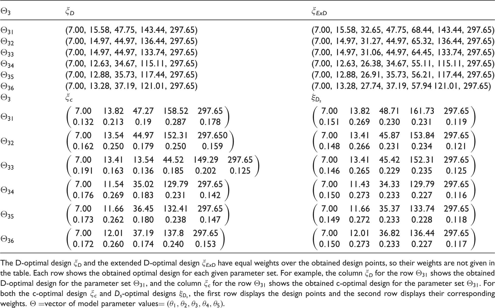
We use the R package Opt5PL and for each vector of nominal values, generate the locally D-optimal designs ξ _D , locally c-optimal designs ξ _c , and locally D _s -optimal designs ${\xi }_{D_s}$ for the 5PL models. The suggested guideline for fitting the 5PL model requires at least six design points, and so one may add two evenly spaced design points between the second and the fourth design points of ξ _D on the log scale, and call this an extended D-optimal design ξ _ExD . The extended D-optimal design has equal weight across the seven design points. Table 7 displays the four types of locally optimal designs including the extended D-optimal designs ξ _ExD found for the six sets of nominal values. For space consideration, we provide the obtained optimal designs for study 2 only. In both studies, the three types of locally optimal designs always contain the endpoints of the range space and the middle points are changed by different optimality criteria and the nominal parameter values.

Table 7.

Four different types of locally optimal designs, ξ_D, ξ_ExD, ξ_c, and ${\xi }_{D_s}$ for the 5PL model for the six sets of parameter values ( ${\Theta }_{31}\sim {\Theta }_{36}$ ) for Study 2.

${\Theta }_3$	ξD	ξExD
${\Theta }_{31}$	(7.00, 15.58, 47.75, 143.44, 297.65)	(7.00, 15.58, 32.65, 47.75, 68.44, 143.44, 297.65)
${\Theta }_{32}$	(7.00, 14.97, 44.97, 136.44, 297.65)	(7.00, 14.97, 31.27, 44.97, 65.32, 136.44, 297.65)
${\Theta }_{33}$	(7.00, 14.97, 44.97, 133.74, 297.65)	(7.00, 14.97, 31.06, 44.97, 64.45, 133.74, 297.65)
${\Theta }_{34}$	(7.00, 12.63, 34.67, 115.11, 297.65)	(7.00, 12.63, 26.38, 34.67, 55.11, 115.11, 297.65)
${\Theta }_{35}$	(7.00, 12.88, 35.73, 117.44, 297.65)	(7.00, 12.88, 26.91, 35.73, 56.21, 117.44, 297.65)
${\Theta }_{36}$	(7.00, 13.28, 37.19, 121.01, 297.65)	(7.00, 13.28, 27.74, 37.19, 57.94 121.01, 297.65)
${\Theta }_3$	ξ c	${\xi }_{D_s}$
${\Theta }_{31}$	$(\begin{array}{ccccc}7.00& \hfill 13.82\hfill & \hfill 47.27\hfill & \hfill 158.52\hfill & \hfill 297.65\hfill \\ 0.132& \hfill 0.213\hfill & \hfill 0.19\hfill & \hfill 0.287\hfill & \hfill 0.178\hfill \end{array})$	$(\begin{array}{ccccc}7.00& \hfill 13.82\hfill & \hfill 48.71\hfill & \hfill 161.73\hfill & \hfill 297.65\hfill \\ 0.151& \hfill 0.269\hfill & \hfill 0.230\hfill & \hfill 0.231\hfill & \hfill 0.119\hfill \end{array})$
${\Theta }_{32}$	$(\begin{array}{ccccc}7.00& \hfill 13.54\hfill & \hfill 44.97\hfill & \hfill 152.31\hfill & \hfill 297.650\hfill \\ 0.162& \hfill 0.250\hfill & \hfill 0.179\hfill & \hfill 0.250\hfill & \hfill 0.159\hfill \end{array})$	$(\begin{array}{ccccc}7.00& \hfill 13.41\hfill & \hfill 45.87\hfill & \hfill 153.84\hfill & \hfill 297.65\hfill \\ 0.148& \hfill 0.266\hfill & \hfill 0.231\hfill & \hfill 0.234\hfill & \hfill 0.121\hfill \end{array})$
${\Theta }_{33}$	$(\begin{array}{cccccc}7.00& \hfill 13.41\hfill & \hfill 13.54\hfill & \hfill 44.52\hfill & \hfill 149.29\hfill & \hfill 297.65\hfill \\ 0.191& \hfill 0.163\hfill & \hfill 0.136\hfill & \hfill 0.185\hfill & \hfill 0.202\hfill & \hfill 0.125\hfill \end{array})$	$(\begin{array}{ccccc}7.00& \hfill 13.41\hfill & \hfill 45.42\hfill & \hfill 152.31\hfill & \hfill 297.65\hfill \\ 0.146& \hfill 0.265\hfill & \hfill 0.229\hfill & \hfill 0.235\hfill & \hfill 0.125\hfill \end{array})$
${\Theta }_{34}$	$(\begin{array}{ccccc}7.00& \hfill 11.54\hfill & \hfill 35.02\hfill & \hfill 129.79\hfill & \hfill 297.65\hfill \\ 0.176& \hfill 0.269\hfill & \hfill 0.183\hfill & \hfill 0.231\hfill & \hfill 0.142\hfill \end{array})$	$(\begin{array}{ccccc}7.00& \hfill 11.43\hfill & \hfill 34.33\hfill & \hfill 129.79\hfill & \hfill 297.65\hfill \\ 0.150& \hfill 0.273\hfill & \hfill 0.233\hfill & \hfill 0.227\hfill & \hfill 0.116\hfill \end{array})$
${\Theta }_{35}$	$(\begin{array}{ccccc}7.00& \hfill 11.66\hfill & \hfill 36.45\hfill & \hfill 132.41\hfill & \hfill 297.65\hfill \\ 0.173& \hfill 0.262\hfill & \hfill 0.180\hfill & \hfill 0.238\hfill & \hfill 0.147\hfill \end{array})$	$(\begin{array}{ccccc}7.00& \hfill 11.66\hfill & \hfill 35.37\hfill & \hfill 133.74\hfill & \hfill 297.65\hfill \\ 0.149& \hfill 0.272\hfill & \hfill 0.233\hfill & \hfill 0.228\hfill & \hfill 0.118\hfill \end{array})$
${\Theta }_{36}$	$(\begin{array}{ccccc}7.00& \hfill 12.01\hfill & \hfill 37.19\hfill & \hfill 137.8\hfill & \hfill 297.65\hfill \\ 0.172& \hfill 0.260\hfill & \hfill 0.174\hfill & \hfill 0.240\hfill & \hfill 0.153\hfill \end{array})$	$(\begin{array}{ccccc}7.00& \hfill 12.01\hfill & \hfill 36.82\hfill & \hfill 136.44\hfill & \hfill 297.65\hfill \\ 0.150& \hfill 0.273\hfill & \hfill 0.233\hfill & \hfill 0.227\hfill & \hfill 0.117\hfill \end{array})$

The D-optimal design ξ _D and the extended D-optimal design ξ _ExD have equal weights over the obtained design points, so their weights are not given in the table. Each row shows the obtained optimal design for each given parameter set. For example, the column ξ _D for the row ${\Theta }_{31}$ shows the obtained D-optimal design for the parameter set ${\Theta }_{31}$ , and the column ξ _c for the row ${\Theta }_{31}$ shows the obtained c-optimal design for the parameter set ${\Theta }_{31}$ . For both the c-optimal design ξ _c and D _s -optimal designs ${\xi }_{D_s}$ , the first row displays the design points and the second row displays their corresponding weights. $\Theta =$ vector of model parameter values $=({\theta }_1,{\theta }_2,{\theta }_3,{\theta }_4,{\theta }_5)$ .

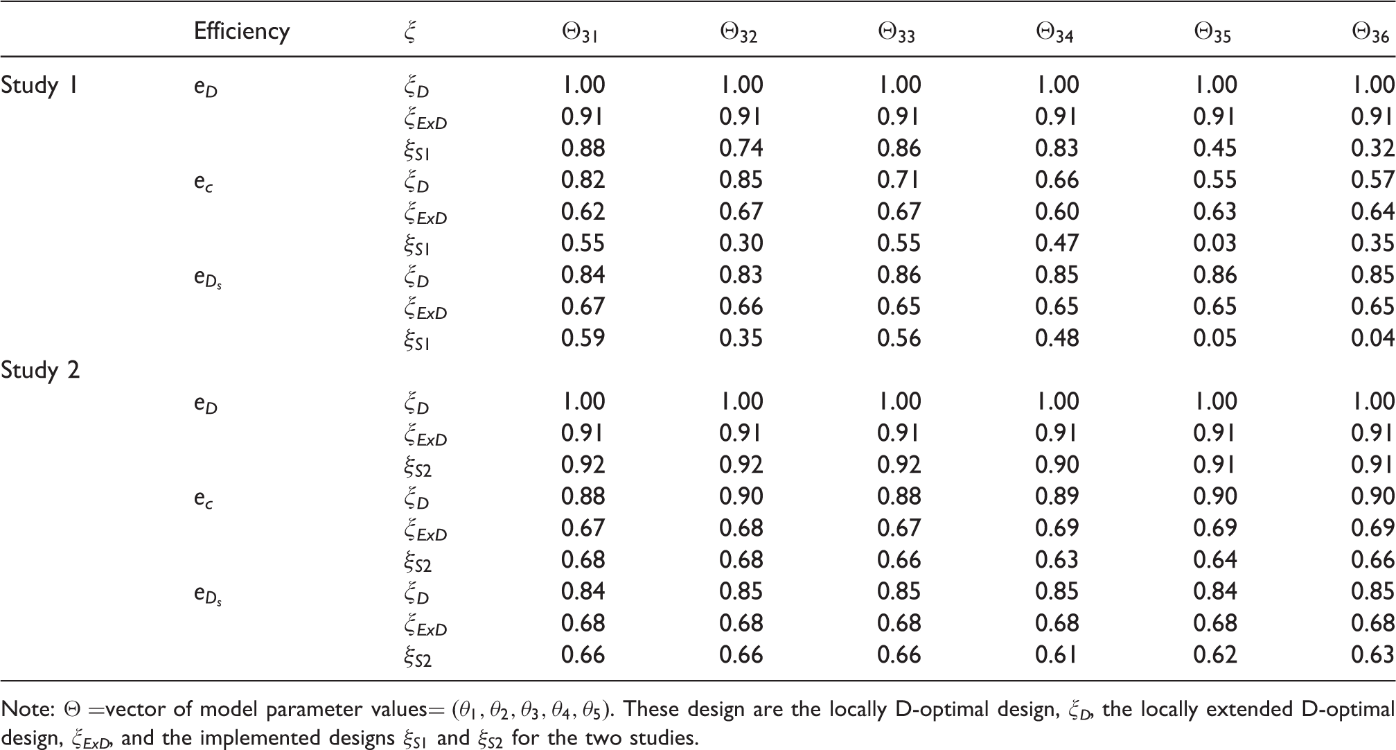
Table 8 shows the performances of the designs ξ _D , ξ _ExD , the implemented design ${\xi }_{S1}$ for study 1 and the implemented design ${\xi }_{S2}$ for study 2 in terms of the three objectives, which are estimating the five parameters in the 5PL model, estimating the EC₅₀ and estimating θ₅. Clearly, the D-optimal designs have 100% D-efficiencies, as shown in the first row in both tables. For the other two objectives, the locally D-optimal designs for both studies still have much higher efficiencies than those provided by the extended design and the implemented designs. The table also shows the extended designs clearly do better than the implemented designs for estimating model parameters. The last two rows in each of the three efficiency categories show that the two implemented designs ${\xi }_{S1}$ and ${\xi }_{S2}$ clearly and substantially underperform and in some case, its D _s -efficiencies for estimating the parameter θ₅ are near 0. For both studies, the extended designs outperform the implemented designs and more so in Study 1. We also observe there is less variation in the efficiencies in Study 2 than in Study 1 across the six sets of nominal values.

Table 8.

Efficiencies of various designs for the 5PL model with different objectives and 6 sets of nominal values for Study 1 and Study 2.

	Efficiency	ξ	${\Theta }_{31}$	${\Theta }_{32}$	${\Theta }_{33}$	${\Theta }_{34}$	${\Theta }_{35}$	${\Theta }_{36}$
Study 1	e D	ξ D	1.00	1.00	1.00	1.00	1.00	1.00
		ξ ExD	0.91	0.91	0.91	0.91	0.91	0.91
		${\xi }_{S1}$	0.88	0.74	0.86	0.83	0.45	0.32
	e c	ξ D	0.82	0.85	0.71	0.66	0.55	0.57
		ξ ExD	0.62	0.67	0.67	0.60	0.63	0.64
		${\xi }_{S1}$	0.55	0.30	0.55	0.47	0.03	0.35
	$e_{D_s}$	ξ D	0.84	0.83	0.86	0.85	0.86	0.85
		ξ ExD	0.67	0.66	0.65	0.65	0.65	0.65
		${\xi }_{S1}$	0.59	0.35	0.56	0.48	0.05	0.04
Study 2
	e D	ξ D	1.00	1.00	1.00	1.00	1.00	1.00
		ξ ExD	0.91	0.91	0.91	0.91	0.91	0.91
		${\xi }_{S2}$	0.92	0.92	0.92	0.90	0.91	0.91
	e c	ξ D	0.88	0.90	0.88	0.89	0.90	0.90
		ξ ExD	0.67	0.68	0.67	0.69	0.69	0.69
		${\xi }_{S2}$	0.68	0.68	0.66	0.63	0.64	0.66
	$e_{D_s}$	ξ D	0.84	0.85	0.85	0.85	0.84	0.85
		ξ ExD	0.68	0.68	0.68	0.68	0.68	0.68
		${\xi }_{S2}$	0.66	0.66	0.66	0.61	0.62	0.63

Note: $\Theta =$ vector of model parameter values $=({\theta }_1,{\theta }_2,{\theta }_3,{\theta }_4,{\theta }_5)$ . These design are the locally D-optimal design, ξ _D , the locally extended D-optimal design, ξ _ExD , and the implemented designs ${\xi }_{S1}$ and ${\xi }_{S2}$ for the two studies.

The efficiencies of the implemented design for estimating EC₅₀ range from 3% to 65% in Study 1 and they range from 63% to 68% in Study 2. The corresponding efficiencies from the extended designs are remarkably stable averaging around 66% for Study 1 and Study 2. In the two studies, the locally D-optimal design does well for estimating the EC₅₀ and θ₅ and average in the mid-1980s for Study 1 and in the high-eighties for Study 2. The overall message from the table is that the extended D-optimal designs appears practically useful and the implemented designs ${\xi }_{S1}$ and ${\xi }_{S2}$ do not when nominal values for the model parameters are misspecified.

6.2 Efficiencies of the implemented designs under mean function misspecification

Many statistical models in immunoassays and bioassays revolve around the 4PL and 5PL models and sometimes the 3PL model. All three models describe a sigmoidal curve for the mean response. Frequently, it is not clear which one of these models is the most appropriate and it is desirable to have a design that works relatively well regardless which one of them holds. We propose a robust locally D-optimal design that can provide well-balanced efficiencies for estimating model parameters in the three models.

We assume the same six sets of possible nominal values in Table 7 for the 5PL model parameters in Study 1 and for each set, simulated data from the 5PL model at the design points of the implemented design ${\xi }_{S1}$ and used them to estimate the model parameters for the 3PL and the 4PL models, respectively. These estimated nominal values are obtained using our nlm R program and they then serve as nominal values for the 3PL and the 4PL models. The same procedure is repeated using ${\xi }_{S2}$ for Study 2 to obtain nominal values for the 3PL and 4PL models for Study 2.

To tackle the model uncertainty issue, we elicit prior probabilities ${\lambda }_1,{\lambda }_2,{\lambda }_3$ for the three models with a higher probability for the more likely model, subject to the probabilities sum to unity. For example, if we believe that the three models are equally plausible, we set ${\lambda }_1={\lambda }_2={\lambda }_3=1/3$ . We then apply our R package and optimize the criterion (5) to obtain a robust D-optimal designs ξ _RoD for each of study. We do not display them for space consideration and note that the robust D-optimal designs always include the two endpoints of the range space.

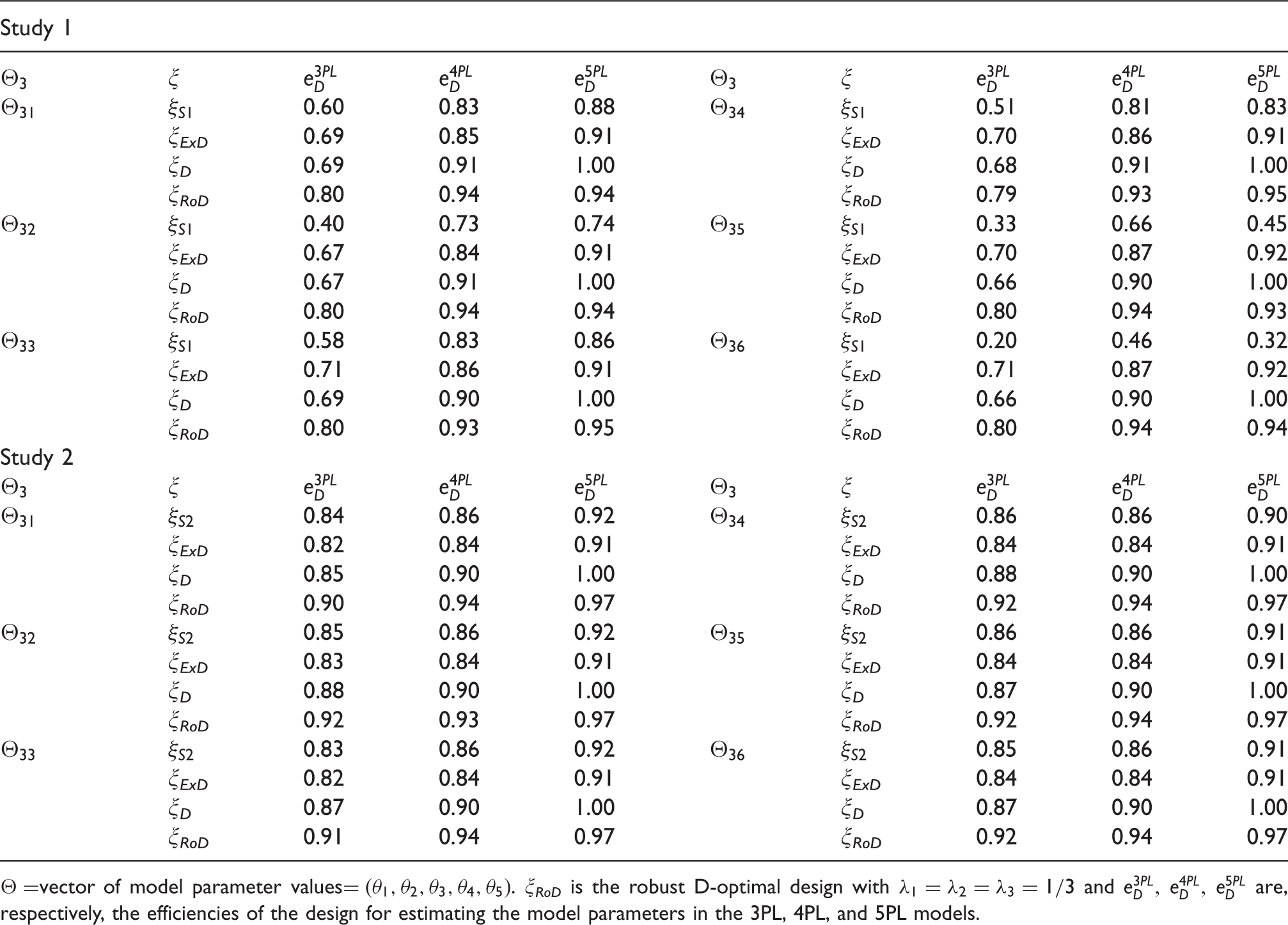
Table 9 shows the D-efficiencies of the designs ${\xi }_{S1},{\xi }_{S2}$ , ξ _ExD , ξ _D , ξ _RoD across the different models $3\mathit{PL},4\mathit{PL}$ and 5PL for each of the six different sets of parameter values for Study 1 and Study 2. The D-efficiencies under the 3PL and 4PL models are calculated using the definition in Section 3.4 assuming one of the three models is the true model and the nominal parameters are the estimated parameters for the 3PL and the 4PL models to obtain the robust D-optimal designs. For Study 1, the implemented design ${\xi }_{S1}$ consistently underperforms relative to the extended design and the robust design by a wide margin in terms of estimating model parameters. For Study 2, the D-efficiencies have a similar pattern but the differences are less dramatic than in Study 1. For both studies, the extended designs generally have satisfactory performance for estimating parameters in the three models and not too different from those provided by the D-optimal designs. The D-optimal design for the 5PL model performs well even when the 3PL or 4PL model is the true model in Study 2 since its lowest D-efficiency across the six sets of nominal values is about 85%; this number drops to about 66% in Study 1. A clear set of results is the D-efficiencies from the robust D-optimal designs are uniformly high for both studies across the six sets of nominal values for the parameters in the 3PL, 4PL and 5PL models. The minimum D-efficiency in Study 1 is about 79% and that in Study 2 is 90%.

Table 9.

D-efficiencies of the four designs, ${\xi }_{S1}$ and ${\xi }_{S2}$ , ξ_ExD, ξ_D, and ξ_RoD for the 3PL, 4PL and 5PL models under the six sets of nominal values for Study 1 and Study 2.

Study 1
${\Theta }_3$	ξ	$e_D^{3\mathit{PL}}$	$e_D^{4\mathit{PL}}$	$e_D^{5\mathit{PL}}$	${\Theta }_3$	ξ	$e_D^{3\mathit{PL}}$	$e_D^{4\mathit{PL}}$	$e_D^{5\mathit{PL}}$
${\Theta }_{31}$	${\xi }_{S1}$	0.60	0.83	0.88	${\Theta }_{34}$	${\xi }_{S1}$	0.51	0.81	0.83
	ξ ExD	0.69	0.85	0.91		ξ ExD	0.70	0.86	0.91
	ξ D	0.69	0.91	1.00		ξ D	0.68	0.91	1.00
	ξ RoD	0.80	0.94	0.94		ξ RoD	0.79	0.93	0.95
${\Theta }_{32}$	${\xi }_{S1}$	0.40	0.73	0.74	${\Theta }_{35}$	${\xi }_{S1}$	0.33	0.66	0.45
	ξ ExD	0.67	0.84	0.91		ξ ExD	0.70	0.87	0.92
	ξ D	0.67	0.91	1.00		ξ D	0.66	0.90	1.00
	ξ RoD	0.80	0.94	0.94		ξ RoD	0.80	0.94	0.93
${\Theta }_{33}$	${\xi }_{S1}$	0.58	0.83	0.86	${\Theta }_{36}$	${\xi }_{S1}$	0.20	0.46	0.32
	ξ ExD	0.71	0.86	0.91		ξ ExD	0.71	0.87	0.92
	ξ D	0.69	0.90	1.00		ξ D	0.66	0.90	1.00
	ξ RoD	0.80	0.93	0.95		ξ RoD	0.80	0.94	0.94
Study 2
${\Theta }_3$	ξ	$e_D^{3\mathit{PL}}$	$e_D^{4\mathit{PL}}$	$e_D^{5\mathit{PL}}$	${\Theta }_3$	ξ	$e_D^{3\mathit{PL}}$	$e_D^{4\mathit{PL}}$	$e_D^{5\mathit{PL}}$
${\Theta }_{31}$	${\xi }_{S2}$	0.84	0.86	0.92	${\Theta }_{34}$	${\xi }_{S2}$	0.86	0.86	0.90
	ξ ExD	0.82	0.84	0.91		ξ ExD	0.84	0.84	0.91
	ξ D	0.85	0.90	1.00		ξ D	0.88	0.90	1.00
	ξ RoD	0.90	0.94	0.97		ξ RoD	0.92	0.94	0.97
${\Theta }_{32}$	${\xi }_{S2}$	0.85	0.86	0.92	${\Theta }_{35}$	${\xi }_{S2}$	0.86	0.86	0.91
	ξ ExD	0.83	0.84	0.91		ξ ExD	0.84	0.84	0.91
	ξ D	0.88	0.90	1.00		ξ D	0.87	0.90	1.00
	ξ RoD	0.92	0.93	0.97		ξ RoD	0.92	0.94	0.97
${\Theta }_{33}$	${\xi }_{S2}$	0.83	0.86	0.92	${\Theta }_{36}$	${\xi }_{S2}$	0.85	0.86	0.91
	ξ ExD	0.82	0.84	0.91		ξ ExD	0.84	0.84	0.91
	ξ D	0.87	0.90	1.00		ξ D	0.87	0.90	1.00
	ξ RoD	0.91	0.94	0.97		ξ RoD	0.92	0.94	0.97

$\Theta =$ vector of model parameter values $=({\theta }_1,{\theta }_2,{\theta }_3,{\theta }_4,{\theta }_5)$ . ξ _RoD is the robust D-optimal design with ${\lambda }_1={\lambda }_2={\lambda }_3=1/3$ and $e_D^{3\mathit{PL}},e_D^{4\mathit{PL}},e_D^{5\mathit{PL}}$ are, respectively, the efficiencies of the design for estimating the model parameters in the 3PL, 4PL, and 5PL models.

7 Conclusions

Our work is the first to address a variety of design issues for the 5PL model. We present optimal designs for estimating model parameters and studying meaningful features of the 5PL model, which can provide a better fit to asymmetric data from bioassays than the 3PL or 4PL models. We compare performance of some of the designs that are recommended for immunoassays and bioassays and show that they may be far from optimum. We suggest designs that are robust to the mean function or nominal values misspecification for the model parameters, and so they provide more accurate statistical inference for the model parameters.

To facilitate users implement optimal designs for the 5PL model, we provide an R package Opt5PL to assess performance of the user-specified designs relative to the optimum, and study robustness properties of a design to various model assumptions. In particular, we show that the locally D-optimal design for estimating the model parameters in the 5PL model is relatively robust to misspecified parameter values for θ₂, θ₃ and θ₅ and also to the form of the mean response. Additionally, we show robust D-optimal designs consistently have high D-efficiencies for estimating model parameters regardless which of the three models 3PL, 4PL or 5PL model holds.

When there are several objectives in the study, the design strategy in Section 3.5 can be used to construct a multiple-objective optimal design that incorporates the relative importance of the objectives. We then formulate a compound criterion by taking a convex combination of the convex criteria with the weights chosen to reflect the relative importance of the criteria. The sought multiple-objective optimal design minimizes the compound criterion. Because the compound criterion is still convex, equivalence theorem can be derived to confirm optimality. Details are in Cook and Wong ¹⁴ and Hyun and Wong, ¹⁵ where a graphical approach is also described to find a multiple-objective optimal design.

We focus on constructing locally optimal designs and future directions for research including finding different types optimal designs for the 5PL model using the maximin, Bayesian and multistage approaches. Another interesting design issue not discussed here is finding optimal designs for the 5PL model when the data has heterogeneous variances. Sometimes bioassays data have heterogeneous variances as the concentration changes. It is not known whether optimal designs discussed here are robust to heteroscedastic errors in the model or whether use of optimal designs based on other efficient estimators such as the maximum quasi likelihood estimator (MqLE) or the extended quasi-likelihood estimator (EQL) provides a better option.

We close with the note that a main role of optimal designs is calibration so that we know what the optimal design is in an ideal situation. In practice, designs should be amended to reflect reality and the needs of the user but not stray too far from the optimum; otherwise the quality of the statistical inference from the study may suffer.

Supplemental Material

Supplemental material for Optimal designs for asymmetric sigmoidal response curves in bioassays and immunoassays

Supplemental Material for Optimal designs for asymmetric sigmoidal response curves in bioassays and immunoassays by Seung Won Hyun, Weng Kee Wong and Yarong Yang in Statistical Methods in Medical Research