A new age-period-cohort model for cancer surveillance research

Abstract

We develop a new age-period-cohort model for cancer surveillance research; the theory and methods are broadly applicable. In the new model, cohort deviations are weighted to account for the variable number of periods that each cohort is observed. Weighting ensures that the fitted rates can be naturally expressed as a function of age × a function of period × a function of cohort. Furthermore, the age, period, and cohort deviations are split into orthogonal quadratic components plus higher-order terms. These decompositions enable powerful combination significance tests of first- and second-order age, period, and cohort effects. The regression parameters of the orthogonal quadratic polynomials (global curvatures) quantify how fast on average the trends in the rates are changing. Importantly, the global curvature for cohort determines the least squares slope of the expected annual percentage changes by age group versus age (local drifts), thereby providing a powerful one-degree-of-freedom test of age-period interactions. We introduce new estimable functions, including age gradients that quantify the rate of change of the longitudinal and cross-sectional age curves at each attained age, and gradient shifts that quantify how the cross-sectional age trend varies by period. We illustrate the new model using nationally representative multiple myeloma incidence. Comprehensive proofs are given in technical appendices. We provide an R package.

1 Introduction

Cancer surveillance research is an observational science of cancer-related rates and risks ascertained in population-based cohorts, notably cancer registries. ¹ In this field, a standard age-period-cohort (APC) model is now well accepted. ² APC models are used to track cancer burden, reveal disparity, provide etiological clues, gauge real-world effectiveness of screening and therapy, quantify natural history and its evolution, and forecast cancer incidence and burden. ³

Our experience analyzing cancer registry data motivated us to develop a next-generation APC model that retains all the good features of the standard model, yet provides new and improved estimable parameters and functions; a natural decomposition of fitted rates into age, period, and cohort effects; and more powerful statistical tests.

In the standard categorical APC model, the age, period, and cohort “deviations” are ensembles of parameters that together measure departures from the overall log-linear temporal trends. ⁴ Our new model incorporates two key innovations. First, cohort deviations are weighted to account for the variable number of periods that each cohort is observed. Because of this modification, the fitted rates can be decomposed into a function of age × a function of period × a function of cohort, without invoking any additional assumptions or constraints. Second, in the new model, the age, period, and cohort deviations are partitioned into orthogonal quadratic components plus higher-order terms. As we will show, the three new “global curvature” parameters corresponding to the quadratic terms for age, period, and cohort, respectively, are intimately connected with fundamental rate patterns and signals that may not be clearly seen when the data are analyzed with the standard model.

We illustrate the new model using cancer incidence data for multiple myeloma (MM) among Black men ascertained through the National Cancer Institute's Surveillance, Epidemiology, and End Results (SEER) program (https://seer.cancer.gov/). SEER is the authoritative source for cancer statistics in the United States (https://seer.cancer.gov/about/). Comprehensive derivations and proofs are presented in technical appendices. We provide an R package.

2 Event rates on a Lexis diagram

APC models parameterize age-specific event rates over time. Formally, the event rates are assumed to be a realization of a Poisson point process over a Lexis diagram, which is a rectangular field with attained age along one axis and calendar period along the other. ⁵ Our convention is the attained age runs along the y-axis and calendar period along the x-axis, to be consistent with outputs from the popular SEERSTAT programs (https://seer.cancer.gov/seerstat/). Individual events and corresponding person-years at risk are summed within a grid of cells defined by equal-width age and period intervals. For any given dataset, we denote the corresponding Lexis diagram as $\mathcal{L}(a_0,p_0,\Delta ,A,P),$ where $a_0$ is the lower limit of the youngest included age group, $p_0$ is the lower limit of the earliest included calendar period, Δ is the common age and period binning interval, A is the total number of age groups, and P is the total number of calendar periods. A Lexis diagram $\mathcal{L}(47,1992,2,19,11)$ for the myeloma data is shown in Figure 1(a).

Figure 1.

Lexis diagram for the myeloma data, displayed as a heat map of observed rates binned into two-year age groups and two-year calendar periods (a). Canonical plot of age-specific rates by birth cohort (b); for each age group, the first point in series corresponds to the earliest period of observation (1992–1993) and last point to the latest year (2013–2014).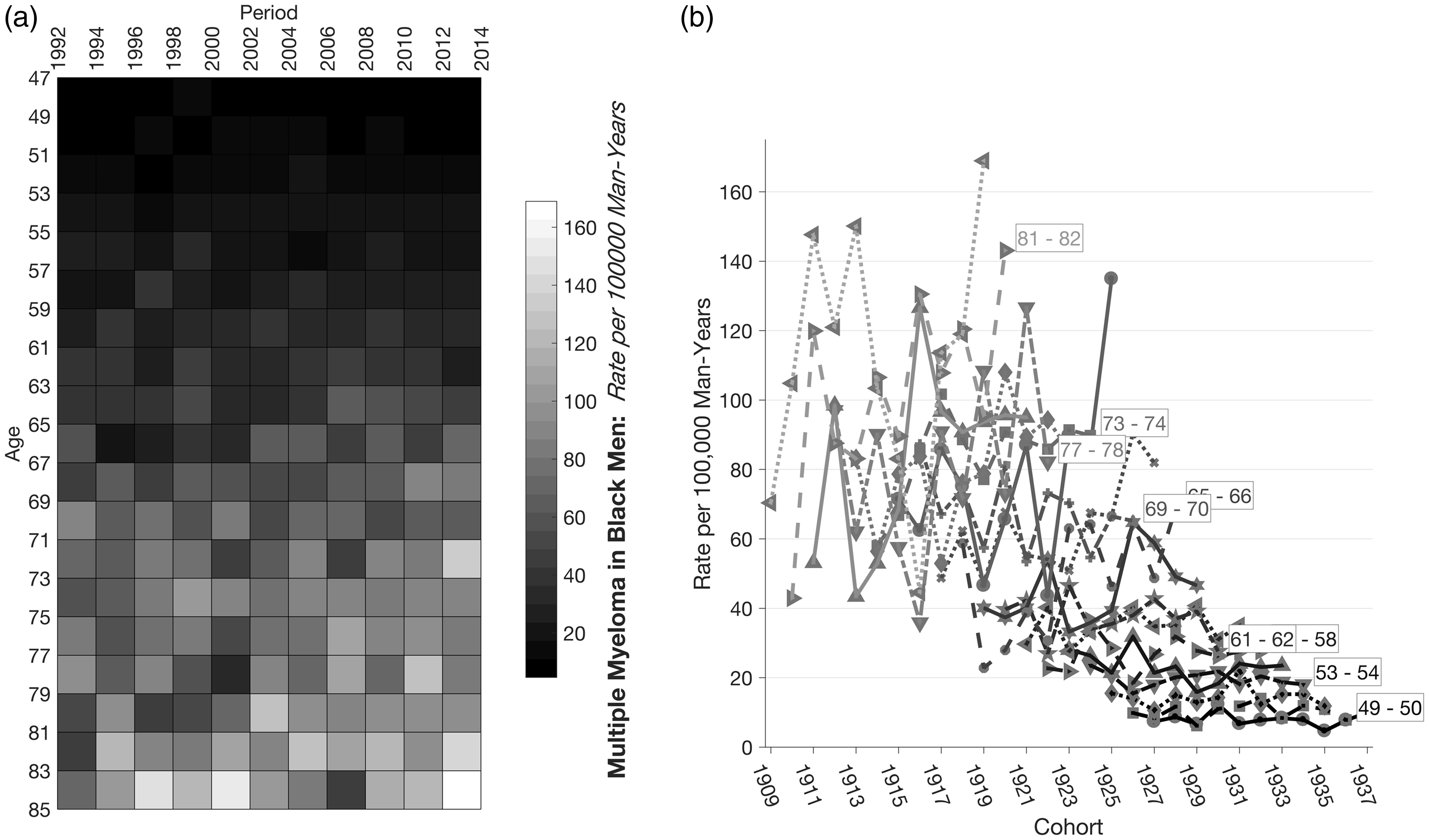

For purposes of modeling, cells along diagonals with slope $-1$ are considered to represent the experience over time of individuals in the same birth-year cohorts. There is always a total of $C=A+P-1$ birth cohorts, from the oldest in the lower left cell through the youngest in the upper right cell.

Each cell can be referenced by values or by indices. Values equal the midpoints of the cell's defining age and period intervals, while indices equal the corresponding sequence number within the Lexis diagram's A consecutive age groups and P consecutive calendar periods.

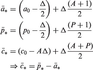
Thus, values, denoted with subscripted *'s, and indices are related as follows

$$\begin{array}{c}{a}_{*}(a)=(a_0-\frac{\Delta }{2})+\Delta a,a=1,\dots ,A{p}_{*}(p)=(p_0-\frac{\Delta }{2})+\Delta p,p=1,\dots ,P{c}_{*}(c)=(c_0-A\Delta )+\Delta c,c=1,\dots ,A+P-1\equiv C\end{array}$$

where $c_0\equiv p_0-a_0$ . From these definitions, it follows that values $c_{*}(p_{*}(p),a_{*}(a))=p_{*}(p)-a_{*}(a)$ and indices $c=p-a+A$ .

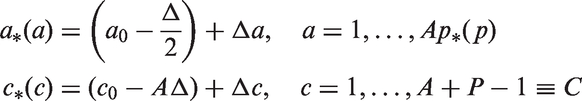
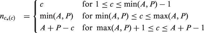
Different cohorts are followed at variable ages and in different periods. The number of cells per cohort is

$$\begin{array}{ccc}{n}_{c_{*}\left(c\right)}& =& \{\begin{array}{c}c for 1\le c\le \text{min}\left(A,P\right)-1\\ \text{min}\left(A,P\right) for \text{min}(A,P)\le c\le \text{max}(A,P)\\ A+P-c for \text{max}\left(A,P\right)+1\le c\le A+P-1\end{array}\end{array}$$

and cohort $c_{*}(c)$ is followed from index age $a_0^c=\text{max}(1,A-c+1)$ through index age $a_1^c=\text{min}(A-c+P,A)$ . When fitting the new model, we use canonical reference values corresponding to the centroid of the Lexis diagram

$$\begin{array}{c}{\overline{a}}_{*}=(a_0-\frac{\Delta }{2})+\Delta \frac{(A+1)}{2}\\ {\overline{p}}_{*}=(p_0-\frac{\Delta }{2})+\Delta \frac{(P+1)}{2}\\ {\overline{c}}_{*}=(c_0-A\Delta )+\Delta \frac{(A+P)}{2}\\ \Rightarrow {\overline{c}}_{*}={\overline{p}}_{*}-{\overline{a}}_{*}\end{array}$$

The rate in each cell per ${10}^5$ person-years is ${\lambda }_{p_{*}{a}_{*}}={10}^5\frac{Y_{p_{*}{a}_{*}}}{O_{p_{*}{a}_{*}}}$ , where $Y_{p_{*}{a}_{*}}$ is the observed number of events and $O_{p_{*}{a}_{*}}$ is the corresponding number of person-years. After the model is fitted we can use arbitrary reference values in estimable functions (Table 1).

Table 1.

Estimable functions of age-period-cohort model parameters.

Estimable function	Equation a
Fitted cohort pattern	$$\begin{array}{c}\mathit{FCP}(c_{*}|a_{*}=a_{*}(a^{\mathit{ref}}))=\text{exp}(({\pi }_L+{\gamma }_L)(c_{*}-{\overline{c}}_{*})+{\theta }_{\gamma }{q}_{c_{*}}^2(c_{*})+{\stackrel{\sim }{\stackrel{\sim }{\gamma }}}_{c_{*}}+\mu +({\alpha }_L+{\pi }_L)(a_{*}(a^{\mathit{ref}})-{\overline{a}}_{*})+{\stackrel{\sim }{\alpha }}_{a_{*}(a^{\mathit{ref}})})\end{array}$$
Cohort rate ratio curve	$$\begin{array}{c}\mathit{CR}{R}_{c_{*}:c_{*}(c^{\mathit{ref}})}=\frac{\mathit{FCP}(c_{*}|a_{*}=a_{*}(a^{\mathit{ref}}))}{\mathit{FCP}(c_{*}(c^{\mathit{ref}})|a_{*}=a_{*}(a^{\mathit{ref}}))}=\text{exp}(({\pi }_L+{\gamma }_L)(c_{*}-c_{*}(c^{\mathit{ref}}))+{\theta }_{\gamma }\{q_{c_{*}}^2(c_{*})-q_{c_{*}}^2(c_{*}(c^{\mathit{ref}}))\}+\{{\stackrel{\sim }{\stackrel{\sim }{\gamma }}}_{c_{*}}-{\stackrel{\sim }{\stackrel{\sim }{\gamma }}}_{c_{*}(c^{\mathit{ref}})}\})\end{array}$$
Fitted temporal trends	$$\begin{array}{c}\mathit{FTT}(p_{*}|a_{*}=a_{*}(a^{\mathit{ref}}))=\text{exp}(({\pi }_L+{\gamma }_L)(p_{*}-{\overline{p}}_{*})+{\theta }_{\pi }{q}_{p_{*}}^2(p_{*})+{\stackrel{\sim }{\stackrel{\sim }{\pi }}}_{p_{*}}+\mu +({\alpha }_L-{\gamma }_L)(a_{*}(a^{\mathit{ref}})-{\overline{a}}_{*})+{\stackrel{\sim }{\alpha }}_{a_{*}(a^{\mathit{ref}})})\end{array}$$
Period rate ratio curve	$$\begin{array}{c}\mathit{PR}{R}_{p_{*}:p_{*}(p^{\mathit{ref}})}=\frac{\mathit{FTT}(p_{*}|a_{*}=a_{*}(a^{\mathit{ref}}))}{\mathit{FTT}(p_{*}(p^{\mathit{ref}})|a_{*}=a_{*}(a^{\mathit{ref}}))}=\text{exp}(({\pi }_L+{\gamma }_L)(p_{*}-p_{*}(p^{\mathit{ref}}))+{\theta }_{\pi }\{q_{p_{*}}^2(p_{*})-q_{p_{*}}^2(p_{*}(p^{\mathit{ref}}))\}+\{{\stackrel{\sim }{\stackrel{\sim }{\pi }}}_{p_{*}}-{\stackrel{\sim }{\stackrel{\sim }{\pi }}}_{p_{*}(p^{\mathit{ref}})}\})\end{array}$$
Longitudinal age curve	$$\begin{array}{c}\mathit{LongAge}(a_{*}|c_{*}=c_{*}(c^{\mathit{ref}}))=\text{exp}(({\alpha }_L+{\pi }_L)(a_{*}-{\overline{a}}_{*})+{\theta }_{\alpha }{q}_{a_{*}}^2(a_{*})+{\stackrel{\sim }{\stackrel{\sim }{\alpha }}}_{a_{*}}+\mu +({\pi }_L+{\gamma }_L)(c_{*}(c^{\mathit{ref}})-{\overline{c}}_{*})+{\stackrel{\sim }{\gamma }}_{c_{*}(c^{\mathit{ref}})})\end{array}$$
Longitudinal age rate ratio curve	$$\begin{array}{c}\mathit{LAR}{R}_{a_{*}:a_{*}(a^{\mathit{ref}})}=\frac{\mathit{LongAge}(a_{*}|c_{*}=c_{*}(c^{\mathit{ref}}))}{\mathit{LongAge}(a_{*}(a^{\mathit{ref}})|c_{*}=c_{*}(c^{\mathit{ref}}))}=\text{exp}(({\alpha }_L+{\pi }_L)(a_{*}-a_{*}(a^{\mathit{ref}}))+{\theta }_{\alpha }\{q_{a_{*}}^2(a_{*})-q_{a_{*}}^2(a_{*}(a^{\mathit{ref}}))\}+\{{\stackrel{\sim }{\stackrel{\sim }{\alpha }}}_{a_{*}}-{\stackrel{\sim }{\stackrel{\sim }{\alpha }}}_{a_{*}(a^{\mathit{ref}})}\})\end{array}$$
Cross-sectional age curve	$$\begin{array}{c}\mathit{CrossAge}(a_{*}|p_{*}=p_{*}(p^{\mathit{ref}}))=\text{exp}(({\alpha }_L-{\gamma }_L)(a_{*}-{\overline{a}}_{*})+{\theta }_{\alpha }{q}_{a_{*}}^2(a_{*})+{\stackrel{\sim }{\stackrel{\sim }{\alpha }}}_{a_{*}}+\mu +({\pi }_L+{\gamma }_L)(p_{*}(p^{\mathit{ref}})-{\overline{p}}_{*})+{\stackrel{\sim }{\pi }}_{p_{*}(p^{\mathit{ref}})})\end{array}$$
Cross-sectional age rate ratio curve	$$\begin{array}{c}\mathit{CAR}{R}_{a_{*}:a_{*}(a^{\mathit{ref}})}=\frac{\mathit{CrossAge}(a_{*}|p_{*}=p_{*}(p^{\mathit{ref}}))}{\mathit{CrossAge}(a_{*}(a^{\mathit{ref}})|p_{*}=p_{*}(p^{\mathit{ref}}))}=\text{exp}(({\alpha }_L-{\gamma }_L)(a_{*}-a_{*}(a^{\mathit{ref}}))+{\theta }_{\alpha }\{q_{a_{*}}^2(a_{*})-q_{a_{*}}^2(a_{*}(a^{\mathit{ref}}))\}+\{{\stackrel{\sim }{\stackrel{\sim }{\alpha }}}_{a_{*}}-{\stackrel{\sim }{\stackrel{\sim }{\alpha }}}_{a_{*}(a^{\mathit{ref}})}\})\end{array}$$

a

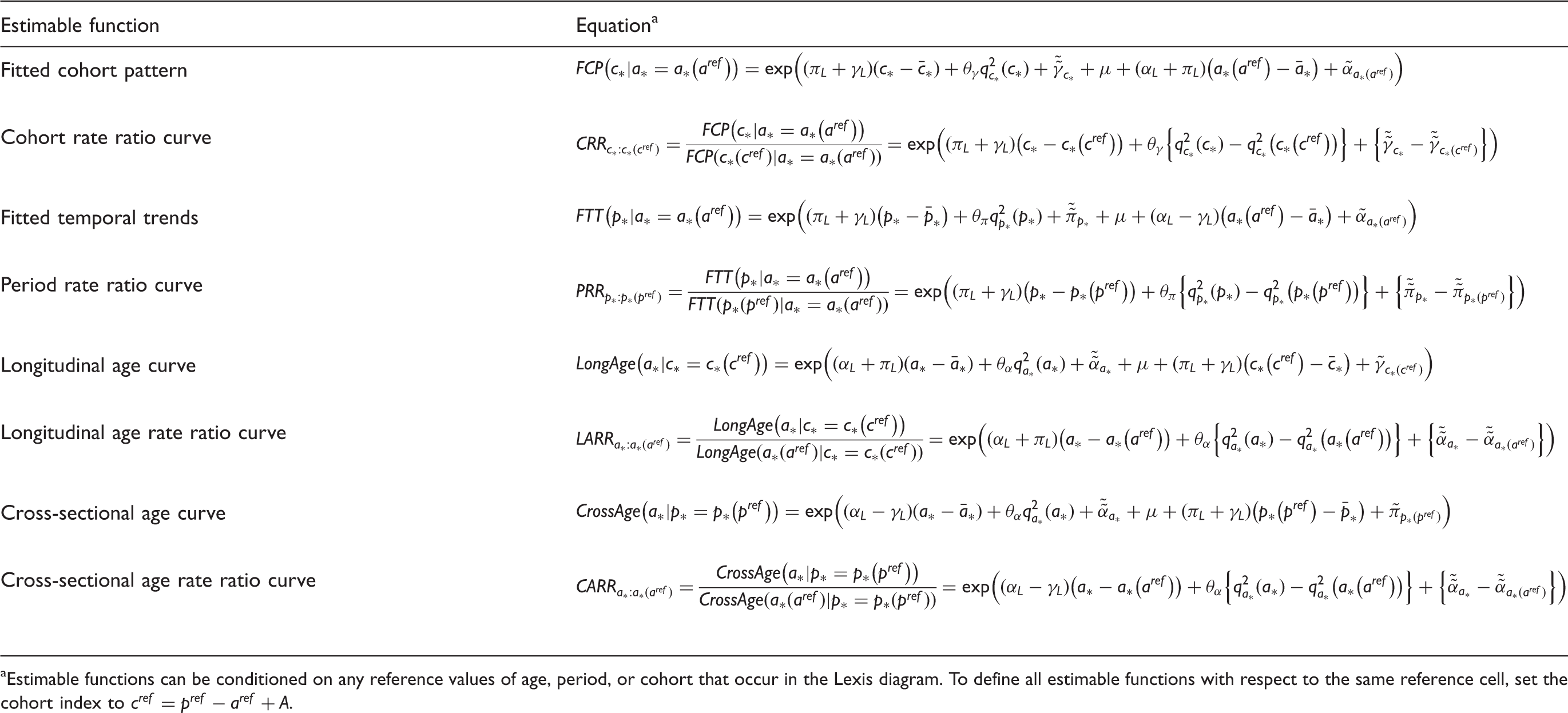
Estimable functions can be conditioned on any reference values of age, period, or cohort that occur in the Lexis diagram. To define all estimable functions with respect to the same reference cell, set the cohort index to $c^{\mathit{ref}}=p^{\mathit{ref}}-a^{\mathit{ref}}+A$ .

3 The standard APC model

For each cell in the Lexis diagram, the expected log rate per 1 person-year is ⁶

$${\rho }_{c_{*}{a}_{*}}=\mathit{ln}({\lambda }_{c_{*},a_{*}})=\mathit{ln}E(\frac{Y_{p_{*}-a_{*},a_{*}}}{O_{p_{*}-a_{*},a_{*}}})=\mu +({\alpha }_L+{\pi }_L)(a_{*}-{\overline{a}}_{*})+({\pi }_L+{\gamma }_L)(c_{*}-{\overline{c}}_{*})+{\stackrel{\sim }{\alpha }}_{a_{*}}+{\stackrel{\sim }{\pi }}_{c_{*}+a_{*}}+{\stackrel{\sim }{\gamma }}_{c_{*}}$$

This is a longitudinal representation when we hold $c_{*}$ fixed and allow $a_{*}$ to vary over the $n_{c_{*}(c)}$ observed age values from $a_{*}(a_0^c)$ through $a_{*}(a_1^c)$ . The equation

$${\rho }_{p_{*}{a}_{*}}=\mathit{ln}({\lambda }_{p_{*},a_{*}})=\mathit{ln}E(\frac{Y_{p_{*},a_{*}}}{O_{p_{*},a_{*}}})=\mu +({\alpha }_L-{\pi }_L)(a_{*}-{\overline{a}}_{*})+({\pi }_L+{\gamma }_L)(p_{*}-{\overline{p}}_{*})+{\stackrel{\sim }{\alpha }}_{a_{*}}+{\stackrel{\sim }{\pi }}_{p_{*}}+{\stackrel{\sim }{\gamma }}_{p_{*}-a_{*}}$$

provides a cross-sectional representation when we define $({\alpha }_L-{\gamma }_L)\equiv ({\alpha }_L+{\pi }_L)-({\pi }_L+{\gamma }_L),$ and hold $a_{*}$ fixed and allow $p_{*}$ to vary over the P observed periods from $p_{*}(1)$ through $p_{*}(P)$ .The fitted values for the two equations are identical. The parameters ${\stackrel{\sim }{\alpha }}_{a_{*}}$ , ${\stackrel{\sim }{\pi }}_{p_{*}}$ and ${\stackrel{\sim }{\gamma }}_{c_{*}}$ are the deviations.

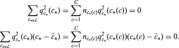
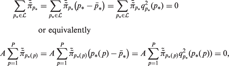
To fit the standard model, we impose six identifiability constraints, two for age, two for period, and two for cohort, in order to make the deviations orthogonal to the intercept and the corresponding log-linear trends. Importantly, in our set-up we impose the constraints over all cells in the Lexis diagram, and not simply over the sequence of A age deviations, P period deviations, and C cohort deviations, which implies that the constraints on the C unique cohort deviations ${\stackrel{\sim }{\gamma }}_{c_{*}(1)},\dots ,{\stackrel{\sim }{\gamma }}_{c_{*}(C)}$ are weighted by $n_{c_{*}(c)}$ .

As described subsequently, this approach insures that the fitted rates can be consistently decomposed into a function of age × a function of period × a function of cohort. We call the quantity $100\times (e^{({\pi }_L+{\gamma }_L)}-1)$ the net drift ⁷ (units are percentage change per calendar year), which is the model-based analogue of the estimated annual percentage change ⁸ (commonly referred to as the EAPC). When there is no possibility of confusion we also refer to the log-linear parameter $({\pi }_L+{\gamma }_L)$ as the net drift. We refer to the quantity $100\times (e^{({\alpha }_L+{\pi }_L)}-1)$ as the longitudinal age trend or LAT, and to $100\times (e^{({\alpha }_L-{\gamma }_L)}-1)$ as the cross-sectional age trend or CAT ⁹ (units of LAT and CAT are percentage change per year of age). Considering the relationship between parameters in the standard versus new model, described subsequently, we now refer to ${\stackrel{\sim }{\alpha }}_{a_{*}}$ , ${\stackrel{\sim }{\pi }}_{p_{*}}$ , and ${\stackrel{\sim }{\gamma }}_{c_{*}}$ as the “complete” age, period, and cohort deviations, respectively.

4 Example: MM in Black men

MM is the most common hematological malignancy among African-American (Black) men, with an estimated lifetime risk of 1.25%. ¹⁰ We extracted MM incidence from the SEER 13 Registries Database (2015 release) ¹¹ for Black men aged 47–84 during calendar years 1992–2013. We tabulated events and man-years within 19 two-year age groups (47–48 through 83–84) and 11 two-year calendar periods (1992–1993 through 2012–2013), which cover 29 nominal birth cohorts centered on birth years 1909 through 1965. In all, there were 3747 incident cases in 10,602,515 man-years.

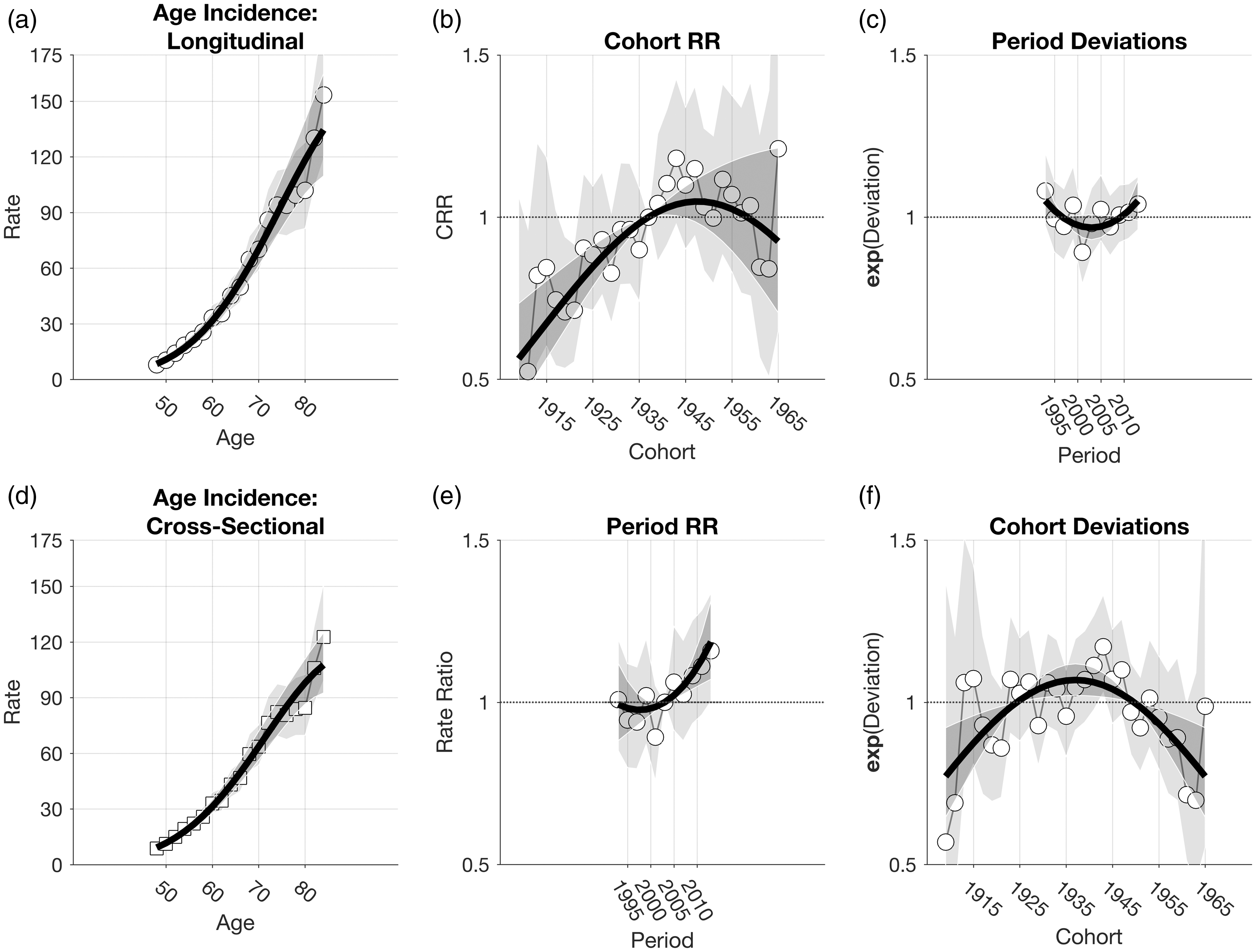
In a “canonical” plot of age-specific incidence rates by birth cohort ¹² (Figure 1(b)), there is a suggestion that incidence is rising in older age groups but has remained comparatively stable in younger age groups. However, the observed rates are “noisy” and simple inspection does not to us suggest any firm conclusions. Outputs from the standard APC model ⁶ (Figure 2) are also quite variable. The net drift of 0.89% per year (95% Confidence Interval [CI]: 0.36–1.42 %/year) is statistically significant (p = 0.001), hence, on average, the rates in Figure 1(b) and the Period and Cohort Rate Ratios in Figure 2(e) and (f) are increasing significantly over birth cohorts and calendar periods, respectively. The LAT of 8.0% per year (95% CI: 7.3–8.7%/year) is highly significant (p ≈ 0). Also, there appears to be some “deceleration” In the cohort deviations circa 1943 (Figure 2(c)) such that incidence increases in successive cohorts through circa 1943 and then decreases (Figure 2(e)), a pattern which is consistent with Figure 1(b). Formally, however, the cohort deviations are not statistically significant (p = 0.499). Overall, our impression is results from the standard model are too noisy to make firm conclusions about temporal effects; it would be appealing to incorporate additional smoothness in the model parameters.

Figure 2.

Estimable functions from the standard APC model fitted to the myeloma data. The reference values are 66 years for age, 2003 for period, and 1937 for birth cohort.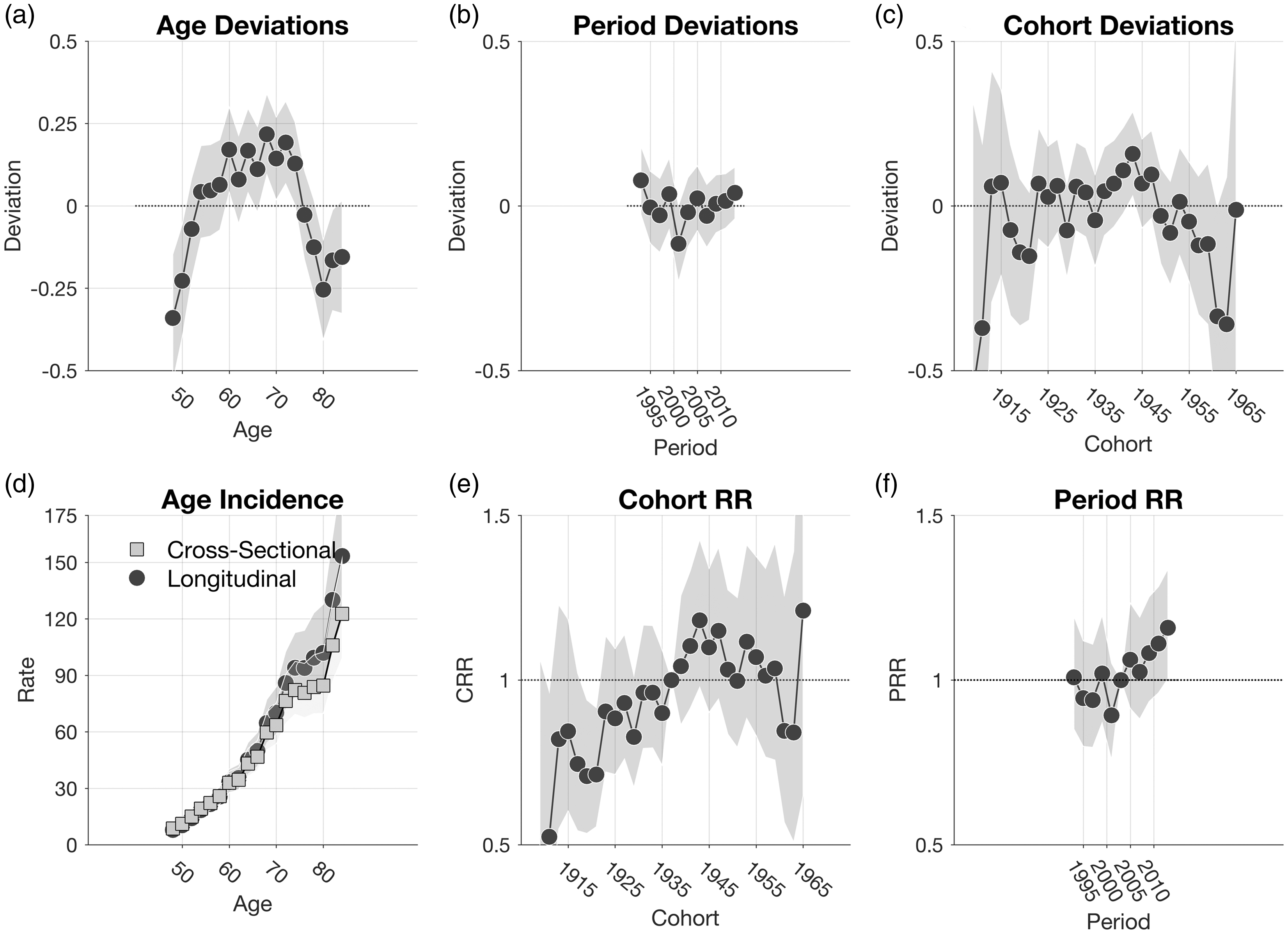

5 The new APC model

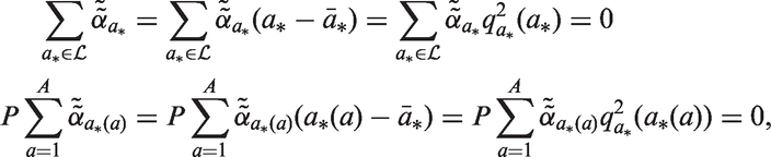
The basic idea is we split the complete deviations 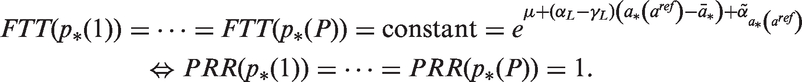${\stackrel{\sim }{\alpha }}_{a_{*}}$ , ${\stackrel{\sim }{\pi }}_{p_{*}}$ , and ${\stackrel{\sim }{\gamma }}_{c_{*}}$ into an orthogonal quadratic component plus higher-order terms,

$$\begin{array}{c}{\stackrel{\sim }{\alpha }}_{a_{*}}={\theta }_{\alpha }{q}_{a_{*}}^2(a_{*})+{\stackrel{\sim }{\stackrel{\sim }{\alpha }}}_{a_{*}}\\ {\stackrel{\sim }{\pi }}_{p_{*}}={\theta }_{\pi }{q}_{p_{*}}^2(p_{*})+{\stackrel{\sim }{\stackrel{\sim }{\pi }}}_{p_{*}}\\ {\stackrel{\sim }{\gamma }}_{c_{*}}={\theta }_{\gamma }{q}_{c_{*}}^2(c_{*})+{{\stackrel{\sim }{\stackrel{\sim }{\gamma }}}_c}_{*}.\end{array}$$

so that

$${\rho }_{c_{*}{a}_{*}}=\mu +({\alpha }_L+{\pi }_L)(a_{*}-{\overline{a}}_{*})+({\pi }_L+{\gamma }_L)(c_{*}-{\overline{c}}_{*})+{\theta }_{\alpha }{q}_{a_{*}}^2(a_{*})+{\theta }_{\pi }{q}_{p_{*}}^2(c_{*}+a_{*})+{\theta }_{\gamma }{q}_{c_{*}}^2(c_{*})+{\stackrel{\sim }{\stackrel{\sim }{\alpha }}}_{a_{*}}+{\stackrel{\sim }{\stackrel{\sim }{\pi }}}_{p_{*}+a_{*}}+{{\stackrel{\sim }{\stackrel{\sim }{\gamma }}}_c}_{*}.$$

The functions $q_{a_{*}}^2(a_{*})$ , $q_{p_{*}}^2(p_{*})$ , and $q_{c_{*}}^2(c_{*})$ are quadratic polynomials that are orthogonal to the intercept and corresponding log-linear trend, and the higher-order terms ${\stackrel{\sim }{\stackrel{\sim }{\alpha }}}_{a_{*}},{\stackrel{\sim }{\stackrel{\sim }{\pi }}}_{p_{*}}$ and ${\stackrel{\sim }{\stackrel{\sim }{\gamma }}}_{c_{*}}$ are each orthogonal to the intercept and the corresponding log-linear and quadratic terms. In our model, orthogonality is defined ¹³ with respect to the usual inner product $〈\mathbf{x}|\mathbf{y}〉=\sum x_i{y}_i.$ The new model has nine constraints in all (Appendix A.1). We will call the parameters ${\theta }_{\alpha },$ ${\theta }_{\pi }$ , and ${\theta }_{\gamma }$ the “global curvature” for age, period, and cohort, respectively.

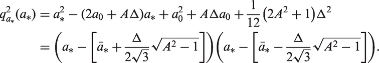
In Appendix A.2 we show that the orthogonal quadratic polynomial for age equals

$$q_{a_{*}}^2(a_{*})=a_{*}^2-[\Delta A+2a_0]a_{*}+[(a_0+\Delta \frac{A}{2}{)}^2-\frac{{\Delta }^2}{12}(A^2-1)],$$

for period equals

$$q_{p_{*}}^2(p_{*})=p_{*}^2-[\Delta P+2p_0]p_{*}+[(p_0+\Delta \frac{P}{2}{)}^2-\frac{{\Delta }^2}{12}(P^2-1)],$$

and for cohort equals

$$q_{c_{*}}^2(c_{*})=c_{*}^2-[\Delta (A+P)+2(c_0-\Delta A)]c_{*}+[(c_0-\Delta A{)}^2+(A+P)\Delta {\overline{c}}_{*}-\frac{{\Delta }^2}{6}\{2A^2+3\mathit{AP}+2P^2-1\}].$$

Each function is completely determined by characteristics of the corresponding Lexis diagram $\mathcal{L}(a_0,p_0,\Delta ,A,P)$ . A design matrix for the new model is presented in Appendix A.3, and fitting the model is described in Appendix A.4.

For the myeloma data, Figure 3 shows the decomposition of the complete deviations for age, period, and cohort into constituent quadratic components plus higher-order terms. Global curvature for age (Figure 3(b)) and cohort (Figure 3(h)) but not period (Figure 3(e)) is statistically significant; the higher-order deviations for age (Figure 3(c)), period (Figure 3(f)), and cohort (Figure 3(i)) are not statistically significant. Hence, most of the variation in myeloma incidence around the intercept μ can be explained by just four of the model's 56 parameters, the two slope parameters $({\alpha }_L+{\pi }_L)$ and $({\pi }_L+{\gamma }_L),$ and the two curvature parameters ${\theta }_{\alpha }$ and ${\theta }_{\gamma }$ .

Figure 3.

Decomposition of complete age, period, and cohort deviations into orthogonal quadratic components plus higher-order terms.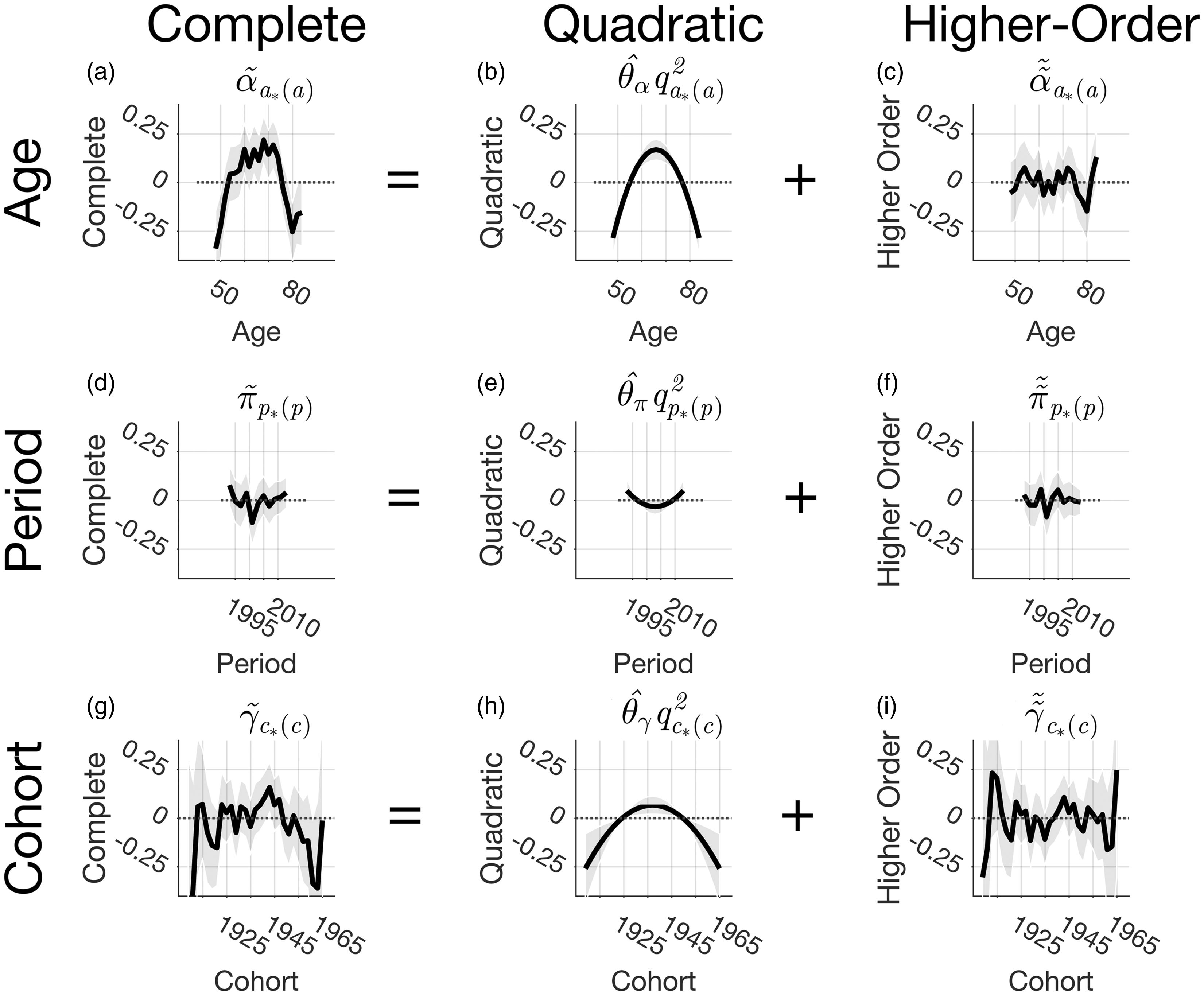

As shown in Appendix A.2, the locations of the roots of the orthogonal quadratic terms are a fixed property of the Lexis diagram. Hence, as shown in Figure 3, panels B, I, and H, the corresponding confidence bands must shrink to 0 at the roots.

6 Estimable functions and the fundamental decomposition principle

Estimable functions are log-linear combinations of identifiable APC coefficients. Estimable functions have been prominently deployed in cancer surveillance studies. In Table 1, we present popular estimable functions of age, period, and cohort, here defined using parameters of the new APC model.

Table 2 shows how estimable functions in Table 1 can be combined to produce equivalent sets of fitted rates. Two of these fundamental decompositions are shown in Figure 4 for the myeloma data, the longitudinal age representation (Figure 4(a) to (c)) and the cross-sectional age representation (Figure 4(d) to (f)). These decompositions yield fitted rates that are identical to the fitted rates obtained directly from the Poisson regression or weighted least squares fit, i.e. to the values of $\hat{\lambda }={10}^5\times \text{exp}(\mathcal{X}\hat{\beta })$ (Appendix A.4). These decompositions will not hold if one substitutes unweighted cohort deviations for the weighted values (Appendix A.7).

Table 2.

Fundamental decompositions of age-period-cohort fitted rates.

Temporality	Time scale	Equation a
Longitudinal	Age	$\lambda (a_{*}|c_{*})=\mathit{LongAge}(a_{*}|c_{*}=c_{*}(c^{\mathit{ref}}))\times \mathit{CR}{R}_{c_{*}:c_{*}(c^{\mathit{ref}})}\times e^{{\stackrel{\sim }{\pi }}_{c_{*}+a_{*}}}$
Longitudinal	Cohort	$\lambda (c_{*}|a_{*})=\mathit{FCP}(c_{*}|a_{*}=a_{*}(a^{\mathit{ref}}))\times \mathit{LAR}{R}_{a_{*}:a_{*}(a^{\mathit{ref}})}\times e^{{\stackrel{\sim }{\pi }}_{c_{*}+a_{*}}}$
Cross-sectional	Age	$\lambda (a_{*}|p_{*})=\mathit{CrossAge}(a_{*}|p_{*}=p_{*}(p^{\mathit{ref}}))\times \mathit{PR}{R}_{p_{*}:p_{*}(p^{\mathit{ref}})}\times e^{{\stackrel{\sim }{\gamma }}_{p_{*}-a_{*}}}$
Cross-sectional	Period	$\lambda (p_{*}|a_{*})=\mathit{FTT}(p_{*}|a_{*}=a_{*}(a^{\mathit{ref}}))\times \mathit{CAR}{R}_{a_{*}:a_{*}(a^{\mathit{ref}})}\times e^{{\stackrel{\sim }{\gamma }}_{p_{*}-a_{*}}}$

a

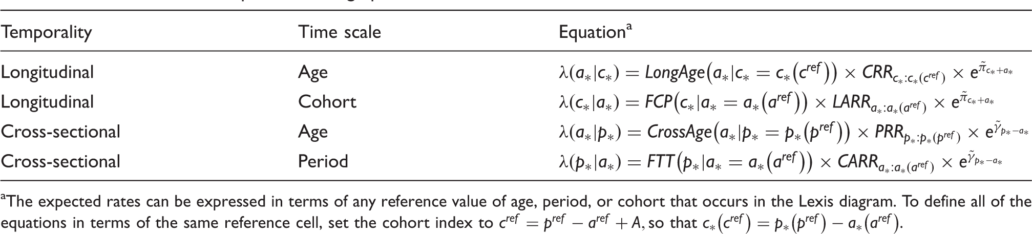
The expected rates can be expressed in terms of any reference value of age, period, or cohort that occurs in the Lexis diagram. To define all of the equations in terms of the same reference cell, set the cohort index to $c^{\mathit{ref}}=p^{\mathit{ref}}-a^{\mathit{ref}}+A,\text{so}\hspace{1em}\text{that}\hspace{1em}{c}_{*}(c^{\mathit{ref}})=p_{*}(p^{\mathit{ref}})-a_{*}(a^{\mathit{ref}})$ .

Figure 4.

Estimable functions of the myeloma data based on new APC model. The bold curve in each panel shows the contributions of the linear and quadratic terms. The reference values are 66 years for age, 2003 for period, and 1937 for birth cohort.

Other useful estimable functions involve finite first and second derivatives of the deviations and estimable functions shown in Table 1. Let

$$\begin{array}{c}{\mathbf{S}}_P=[\begin{array}{c}1\\ \begin{array}{c}2\\ :\end{array}\\ P\end{array}]\text{\hspace{1em}and\hspace{1em}}{1}_P\equiv [\begin{array}{c}1\\ :\\ 1\end{array}{]}_{P\times 1}\end{array}$$

As described in Appendix B, the gradient of the cross-sectional age curve on the logarithmic scale equals

$$\begin{array}{c}{\stackrel{·}{\rho }}_{\mathit{CROSS}}({\mathbf{a}}_{*}|p_{*}=p_{*}(p^{\mathit{ref}}))={\mathbf{G}}_{(A,\Delta )}[{\rho }_{\mathit{CROSS}}(a_{*}(a)|p_{*}=p_{*}(p^{\mathit{ref}})){]}_{a_{*}(1)}^{a_{*}(A)}\\ =({\alpha }_L-{\gamma }_L)1_{A-1}+2{\theta }_{\alpha }\Delta \{{\mathbf{S}}_{A-1}-\frac{A}{2}{1}_{A-1}\}+{\mathbf{G}}_{(A,\Delta )}{\stackrel{\sim }{\sim }\alpha }_{a_{*}},\end{array}$$

where ${\mathbf{G}}_{(A,\Delta )}$ is a finite difference operator. The gradient of the longitudinal age curve has the same form with $({\alpha }_L-{\gamma }_L)$ replaced by $({\alpha }_L+{\pi }_L)$ .

In the literature, there has been considerable interest in second differences of cohort deviations.^14,15 These can be extracted from ${{\stackrel{\sim }{\gamma }}_c}_{*}$ using a finite second difference operator ${\mathit{G}}_C^{\Delta }{\hspace{0.17em}}^2$ . It is worth noting (Appendix A.6) that second differences of the traditional unweighted cohort deviations are identical to second differences of the weighted values.

7 Combination hypothesis tests of period and cohort deviations

A fundamental question is whether period or cohort effects influence the rates over and above log-linear influences captured through the net drift parameter $({\pi }_L+{\gamma }_L)$ . The standard model's approach is to calculate omnibus Chi-square tests with $(P-2)$ degrees of freedom ( $\mathit{df}$ ) and $(C-2)\hspace{1em}\mathit{df},$ respectively. A problem is these tests can be under-powered for rare outcomes or granular data. We seek a test that is sensitive to signals in the quadratic or higher-order components alone, or simultaneously. Using the new model, we propose to use Tippett's Method ¹⁶ to construct a new p-value combination test of significance of the complete period deviations, i.e. quadratic and/or higher-order period signals. Tippett's method is used to combine k independent statistical tests into an overall test of the global null hypothesis $H_0$ . Tippett's method rejects $H_0$ at overall significance level α if any of $P_1,\dots ,P_k\le \alpha \text{'}=1-(1-\alpha {)}^{1/k}$ . In practice, we use the conservative approximation $\frac{\alpha }{k}<1-(1-\alpha {)}^{1/k}$ , so that the combination test is

$$T_{\alpha }^{\stackrel{\sim }{\pi }}=min(2P^{{\theta }_{\pi }},2P^{\stackrel{\sim }{\stackrel{\sim }{\pi }}},1),$$

where $P^{{\theta }_{\pi }}$ is the p value for the 1-df Wald Chi-square test of global curvature for period, and $P^{\stackrel{\sim }{\stackrel{\sim }{\pi }}}$ is the p value for the $(P-3)$ df Wald Chi-square test of higher-order period deviations.

Similarly, we propose a new p-value combination test for the complete cohort deviations

$$T_{\alpha }^{\stackrel{\sim }{\gamma }}=min(2P^{{\theta }_{\gamma }},2P^{\stackrel{\sim }{\stackrel{\sim }{\gamma }}},1),$$

where $P^{{\theta }_{\gamma }}$ is the p value for the 1-df Wald Chi-square test of global curvature for cohort, and $P^{\stackrel{\sim }{\stackrel{\sim }{\gamma }}}$ is the p value for the $(C-3)$ df Wald Chi-square test of higher-order cohort deviations.

For the myeloma data, the standard Wald test for period deviations is ${\chi }_9^2=6.75,P=0.664$ , and the new composite test is $\text{min}(2\times 0.0987,2\times 0.8157,1)=0.1973$ , so neither test is significant. The standard Wald test for cohort deviations is ${\chi }_{27}^2=26.36,P=0.499$ , and the new composite test is $\text{min}(2\times 0.0042,2\times 0.8291,1)=0.0084$ , so the new test clearly identifies a signal that is missed by the old test.

8 Combination hypothesis tests of period and cohort rate ratios

A related question is whether there is any association whatsoever of the rates with calendar period. Using the estimable functions defined in Table 1, under $H_0:$ constant period rate ratios

$$\begin{array}{c}\mathit{FTT}(p_{*}(1))=\dots =\mathit{FTT}(p_{*}(P))=\text{constant}=e^{\mu +({\alpha }_L-{\gamma }_L)(a_{*}(a^{\mathit{ref}})-{\overline{a}}_{*})+{\stackrel{\sim }{\alpha }}_{a_{*}(a^{\mathit{ref}})}}\\ \iff \mathit{PRR}(p_{*}(1))=\dots =\mathit{PRR}(p_{*}(P))=1.\end{array}$$

a p-value combination test of this hypothesis based on Tippett's method is

$$T_{\alpha }^{\mathit{FTT}({\mathbf{p}}_{*})}\equiv T_{\alpha }^{\mathit{PRR}({\mathbf{p}}_{*})}=min(3P^{({\pi }_L+{\gamma }_L)},3P^{{\theta }_{\pi }},3P^{\stackrel{\sim }{\stackrel{\sim }{\pi }}},1).$$

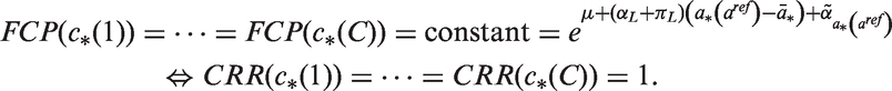
Similarly, under $H_0:$ constant cohort rate ratios

$$\begin{array}{c}\mathit{FCP}(c_{*}(1))=\dots =\mathit{FCP}(c_{*}(C))=\text{constant}=e^{\mu +({\alpha }_L+{\pi }_L)(a_{*}(a^{\mathit{ref}})-{\overline{a}}_{*})+{\stackrel{\sim }{\alpha }}_{a_{*}(a^{\mathit{ref}})}}\\ \iff \mathit{CRR}(c_{*}(1))=\dots =\mathit{CRR}(c_{*}(C))=1.\end{array}$$

a p-value combination test for this hypothesis is

$$T_{\alpha }^{\mathit{FCP}({\mathbf{c}}_{*})}\equiv T_{\alpha }^{\mathit{CRR}({\mathbf{c}}_{*})}=min(3P^{({\pi }_L+{\gamma }_L)},3P^{{\theta }_{\gamma }},3P^{\stackrel{\sim }{\stackrel{\sim }{\gamma }}},1).$$

For the myeloma data, the standard Wald test for period rate ratios is ${\chi }_{10}^2=19.82,P=0.0310$ , and the new combination test is $\text{min}(3\times 0.0001,3\times 0.0987,3\times 0.8157,1)=0.0003$ , thus both tests are significant but the new test much more so. The standard Wald test for cohort rate ratios is ${\chi }_{28}^2=37.67,P=0.1049$ , and the new combination test is $\text{min}(3\times 0.0001,3\times 0.0042,3\times 0.8291,1)=0.003$ , so the new test clearly identifies a signal that is missed by the old test.

9 Power of Wald tests versus combination tests: simulation study

We carried out a simulation study to confirm the level-correctness of our tests and to gauge the potential real-world power gains (if any) obtainable using the new combination tests. We used point estimates from the myeloma data's APC model to define a baseline scenario, and simulated Poisson counts under the baseline and alternative scenarios.

We set $\alpha =0.05$ for all tests. To assess the performance of tests of cohort effects, we multiplied both ${\theta }_{\gamma }$ and ${\stackrel{\sim }{\stackrel{\sim }{\gamma }}}_c$ by 0, 0.5, 0.75, or 1, for two total sample sizes, $1y_{++}\hspace{1em}\mathit{or}\hspace{1em}2y_{++}$ , where $y_{++}\equiv 3,747$ is the total observed number of cases. We used the same design to assess the performance of tests of period effects, except we scaled ${\theta }_{\pi }$ and ${\stackrel{\sim }{\stackrel{\sim }{\pi }}}_p$ rather than ${\theta }_{\gamma }$ and ${\stackrel{\sim }{\stackrel{\sim }{\gamma }}}_c$ .

For cohort effects (Figure 5(a) and (b)), both the Wald tests and the combination tests are level correct for both ${\stackrel{\sim }{\gamma }}_c$ (cohort deviations; Figure 5(a)) and cohort rate ratios (CRR; Figure 5(b)). The combination tests are appreciably more powerful; at the observed sample size the power gains are around 5 to 10 percentage points. For period effects (Figure 5(c) and (d)), as expected, both the Wald tests and the combination tests are level correct for both ${\stackrel{\sim }{\pi }}_p$ (period deviations; Figure 5(c)) and period rate ratios (PRR; Figure 5(d)). The combination tests have slightly higher power or are on par.

Figure 5.

Simulation results assessing Type-I error rates and power of Wald versus combination tests of complete cohort deviations (a); cohort rate ratios (CRR) (b); complete period deviations (c); period rate ratios (PRR) (d). See text for details.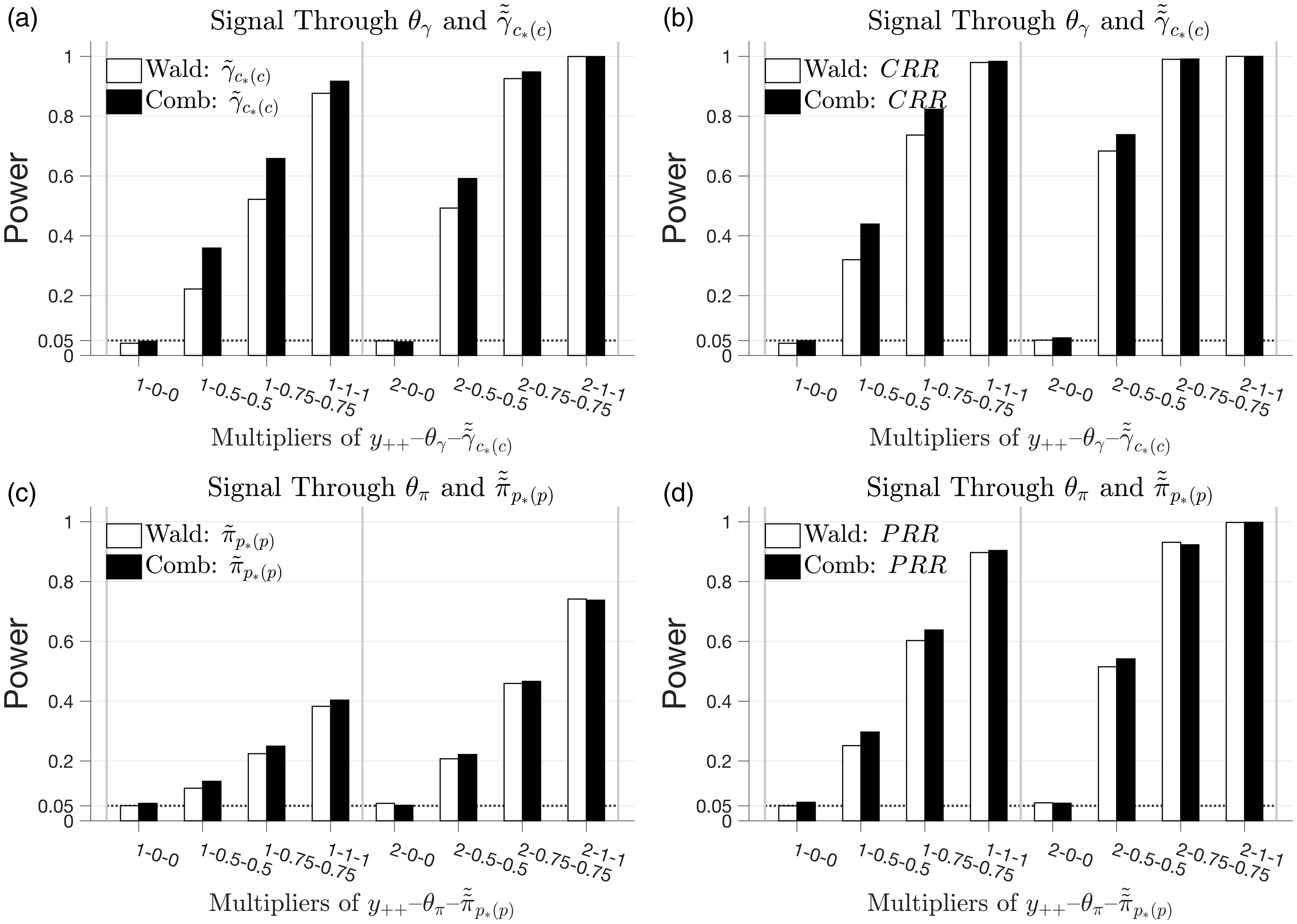

10 Local drifts

Local drifts are model-based estimates of annual percentage changes by age group. ⁶ Departures of local drifts from the overall net drift are a consequence of cohort deviations, hence local drifts quantify the heuristic that cohort effects represent an age interaction over time. Local drifts can be constructed by sliding a window of bandwidth P through the cohort deviations and extracting the least squares slopes, and then adding these “deflection” terms to the overall net drift.

Formally, the cross-sectional age-specific rates over time equal

$$\rho (p_{*}|a_{*}=a_{*}(a))=({\pi }_L+{\gamma }_L)(p_{*}-{\overline{p}}_{*})+{\stackrel{\sim }{\gamma }}_{p_{*}-a_{*}(a)}+{\stackrel{\sim }{\pi }}_{p_{*}}+\mu +({\alpha }_L-{\gamma }_L)(a_{*}(a)-{\overline{a}}_{*})+{\stackrel{\sim }{\alpha }}_{a_{*}(a)}.$$

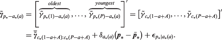
The sub-vector of P complete cohort deviations belonging to age group 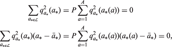$a_{*}(a)$ can be regressed on period (vectors denoted by bold-face) yielding the identity

$$\begin{array}{c}{\stackrel{\sim }{\gamma }}_{p_{*}-a_{*}(a)}=[\stackrel{\mathit{oldest}}{\overbrace{{\stackrel{\sim }{\gamma }}_{p_{*}(1)-a_{*}(a)}}},\dots ,\stackrel{\mathit{youngest}}{\overbrace{{\stackrel{\sim }{\gamma }}_{p_{*}(P)-a_{*}(a)}}}]\text{'}=[{\stackrel{\sim }{\gamma }}_{c_{*}(1-a+A)},\dots ,{\stackrel{\sim }{\gamma }}_{c_{*}(P-a+A)}]\text{'}\\ ={\overline{\stackrel{\sim }{\gamma }}}_{c_{*}(1-a+A):c_{*}(P-a+A)}+{\delta }_{a_{*}(a)}({\mathbf{p}}_{*}-{\overline{\mathbf{p}}}_{*})+\epsilon {\mathbf{p}}_{\mathbf{*}}\mathbf{|}{\mathbf{a}}_{\mathbf{*}}(\mathbf{a}).\end{array}$$

As we move from one age group to the next, we slide along by one birth cohort. We can calculate the ensemble of A deflections 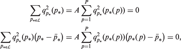${\delta }_{a_{*}(a)}$ as follows. Vector

$${\mathbf{L}}_{1\times P}^{\Delta }=\frac{12}{\Delta (P-1)P(P+1)}({\mathbf{S}}_P-\frac{P+1}{2}{1}_P)\text{'}$$

extracts the least squares slope for any vector of ordinates of length P that are evenly spaced by Δ units apart. Hence, matrix

$$\begin{array}{c}{\mathbf{K}}_{(A,C)}^{\Delta }=[\begin{array}{cc}\{0_{(1)}& \hfill \dots \begin{array}{cc}{0}_{(A-1)}\}& \hfill {\mathbf{L}}_{1\times P}^{\Delta }\hfill \end{array}\hfill \\ \{0_{(1)}& \hfill \dots 0_{(A-2)}\}\hfill & \hfill \begin{array}{cc}{\mathbf{L}}_{1\times P}^{\Delta }& \hfill 0\hfill \end{array}\hfill \\ \begin{array}{c}:\\ \begin{array}{c}0\\ {\mathbf{L}}_{1\times P}^{\Delta }\end{array}\end{array}& \hfill \begin{array}{c}:\\ \begin{array}{c}{\mathbf{L}}_{1\times P}^{\Delta }\\ \{0_{(1)}\dots \end{array}\end{array}\hfill & \hfill \begin{array}{cc}\{0_{(1)}& \hfill \begin{array}{c}:\\ \dots \begin{array}{c}{0}_{(A-2)}\}\\ 0_{(A-1)}\}\end{array}\end{array}\hfill \end{array}\hfill \end{array}]\end{array}$$

extracts from the complete cohort deviations all A deflection terms for the youngest through the oldest age groups,

$${\mathbf{K}}_{(A,C)}^{\Delta }{\stackrel{\sim }{\gamma }}_{C\times 1}={\mathbf{\delta }}_{A\times 1}.$$

As shown in Appendix A.5, under the standard model the local drifts equal

$$[({\pi }_L+{\gamma }_L{)}_{a_{*}(a)}]=({\pi }_L+{\gamma }_L)·1_A+{\mathbf{K}}_{(A,C)}^{\Delta }{\stackrel{\sim }{\gamma }}_{C\times 1}=({\pi }_L+{\gamma }_L)·1_A+{\mathbf{\delta }}_{A\times 1},$$

while under the new model the local drifts equal

$$[({\pi }_L+{\gamma }_L{)}_{a_{*}(a)}]=({\pi }_L+{\gamma }_L)·1_A-2{\theta }_{\gamma }\Delta ({\mathbf{S}}_A-\frac{A+1}{2}{1}_A)+{\mathbf{K}}_{(A,C)}^{\Delta }{\stackrel{\sim }{\sim }\gamma }_{C\times 1}.$$

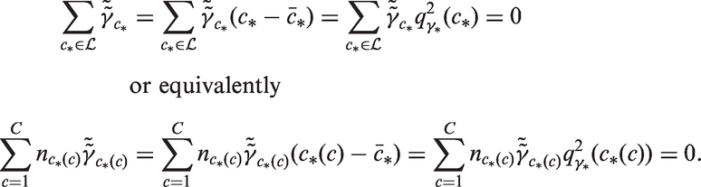
Thus, the least squares slope of the local drifts with respect to age is determined by the global curvature for cohort. When ${\theta }_{\gamma }>0$ and ${\stackrel{\sim }{\sim }\gamma }_{C\times 1}$ is comparatively small, as we move from older through younger cohorts the deflections change sign from negative values that apply to the older age groups $a_{*}(a)>{\overline{a}}_{*}$ to positive values for the younger age groups $a_{*}(a)<{\overline{a}}_{*}$ . Conversely, when ${\theta }_{\gamma }<0$ , the deflections have positive values for older age groups and negative values for younger age groups.

Figure 6 presents local drifts for the myeloma data. For context, canonical plots of age-specific rates over time (Figures 6(a) and 1(b)) suggest that perhaps the rates are increasing in older age groups and are stable or perhaps decreasing in younger age groups. Local drifts from the standard model support this conclusion (Figure 6(b)), but the estimates are uncertain. The new model (Figure 6(c)) confirms that the Local drifts indeed increase consistently with age. On average across ages 45–84, the net drift increases by $100\times (e^{-2{\theta }_{\gamma }}-1)=0.083\%$ per calendar year per year of age (95% CI: $0.03-0.14\%/Y{r}^2$ ). This relatively small increase in drift per single-year-of-age accumulates over the age range. Incidence is essentially flat among men aged 50 years, but among men aged 80 years, the incidence is significantly increasing by 2% per year.

Figure 6.

Local drifts of the myeloma data. (a) Canonical plot of age-specific rates over time (age binned into eight-year groups); (b) estimated annual percentage change per calendar year by age group (local drifts) estimated using standard APC model; (c) local drifts estimates from new APC model.

An important point is local drifts are cross-sectional quantities, and the same cross-sectional values hold whether we condition on age and examine the rates over calendar periods or we condition on calendar periods and examine the rates across age groups. In Appendix C, we show that the log-linear slopes of the cross-sectional age-specific rates within calendar periods equal

$$[({\alpha }_L-{\gamma }_L{)}_{p_{*}(p)}]=({\alpha }_L-{\gamma }_L)·1_P-2{\theta }_{\gamma }\Delta ({\mathbf{S}}_P-\frac{P+1}{2}{1}_P)-{\mathbf{K}}_{(P,C)}{\stackrel{\sim }{\sim }\gamma }_{C\times 1},$$

where matrix ${\mathbf{K}}_{(P,C)}$ slides a length P window through a length C sequence of ordinates evenly spaced by Δ units apart and extract the least squares slope. We call these quantities “Gradient Shifts”. Thus, both the slope of the local drifts over age groups and the slope of the gradient shifts over calendar periods are equal to $-2{\theta }_{\gamma }$ .

11 Local drifts tests

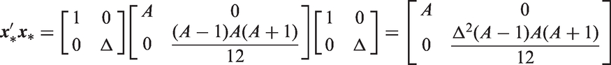
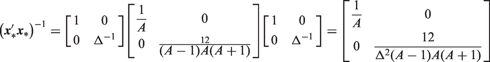
When testing for significance of the local drifts using the standard model, we often rely on an omnibus Wald statistic. The null hypothesis is that all local drifts are equal to the overall net drift, which is true if and only if ${\mathbf{\delta }}_{A\times 1}=0_{A\times 1}$ . By the Delta method

$${\mathit{V}}_{{\mathit{\delta }}_{A\times 1}}={\mathit{K}}_{\left(A, C\right)}^{\Delta }{\mathit{V}}_{{\tilde{\gamma }}_{C\times 1}}{\mathit{K}}_{\left(A, C\right)}^{\Delta }{\text{'}}^{,}$$

hence the Wald test statistic is

$$\begin{array}{c}{W}_{\delta }={\mathbf{\delta }}_{A\times 1}{\mathit{\text{'}}\mathbf{V}}_{{\mathbf{\delta }}_{A\times 1}}^{-}{\mathbf{\delta }}_{A\times 1}\sim {\mathbf{\chi }}_{\mathit{df}}^2\mathit{df}=\text{rank}({\mathbf{V}}_{{\mathbf{\delta }}_{A\times 1}})\end{array}.$$

As shown in Appendix A.5, when the Lexis diagram is rectangular $(A\ne P)$ , ${\mathbf{V}}_{{\mathbf{\delta }}_{A\times 1}}$ is full rank and $\mathit{df}=A$ . However, when the Lexis diagram is square $(A=P)$ , ${\displaystyle \sum _{a=1}^A}{\delta }_a=0$ , hence $\mathit{df}=A-1$ . In other words, when the Lexis diagram is square we lose one degree of freedom and thereby gain a small increase in power. In practice, to calculate the test when $A=P$ , we leave out one component of ${\mathbf{\delta }}_{A\times 1}$ so that the corresponding reduced variance-covariance matrix has full rank.

The new model offers a 1-degree-of-freedom test. Clearly, if ${\theta }_{\gamma }\ne 0$ then ${\mathbf{\delta }}_{A\times 1}\ne 0_{A\times 1}$ . Hence, a 1-degree-of-freedom test evaluates $H_0:{\theta }_{\gamma }=0$ . The test can be carried out using standard outputs from the model fit, i.e. the coefficient ${\hat{\theta }}_{\gamma }$ and its variance $\mathit{Var}({\hat{\theta }}_{\gamma })$ ; the 1 degree of freedom test is simply $W_{{\theta }_{\gamma }}=\frac{{\hat{\theta }}_{\gamma }^2}{\mathit{Var}({\hat{\theta }}_{\gamma })}$ , which is distributed ${\chi }_1^2$ under $H_0$ .

In principle, one could construct a combination test $min(2P^{{\theta }_{\gamma }},2P^{{\mathbf{K}}_{(A,C)}^{\Delta }{\stackrel{\sim }{\sim }\gamma }_{C\times 1}},1),$ but we have not done so because it is difficult to interpret the third-order effects ${\mathbf{K}}_{(A,C)}^{\Delta }{\stackrel{\sim }{\sim }\gamma }_{C\times 1}$ . Instead, we construct the combination test $T_{\alpha }^{\mathit{LocalDrifts}({\mathbf{a}}_{*})}=min(2P^{W_{{\theta }_{\gamma }}},P^{W_{\delta }},1)$ . The test may be conservative because the component tests are dependent.

For the myeloma data, the Omnibus Wald Test is ${\chi }_{19}^2=19.79,P=0.4072$ , and the new 1-degree-of-freedom test is ${\chi }_1^2=8.19,P=0.0042$ , so the new test clearly identifies a signal that is missed by the old test. The combination test statistic is 0.0084, also highly significant.

12 Power of local drifts tests: simulation study

We carried out a simulation study of our new 1- degree-of-freedom (1-df ) and combination tests of local drifts, versus the standard Omnibus test. Our aim was to assess the level-correctness of our tests and to gauge the potential real-world power gains (if any) obtainable using the new tests, when the local drift signals arise from quadratic or higher-order cohort effects alone or simultaneously. As before, we used point estimates from the myeloma data's APC model to define a baseline scenario.

To assess the performance of the drifts tests, we considered three situations. First, ${\stackrel{\sim }{\sim }\gamma }_c\equiv 0$ and ${\theta }_{\gamma }=0{\theta }_{\gamma ,},\hspace{1em}0.5{\theta }_{\gamma },1{\theta }_{\gamma }$ , $\text{or}\hspace{1em}1.5{\theta }_{\gamma }$ , hence all the signal (if any) is coming through the global curvature for cohort. Second, ${\theta }_{\gamma }\equiv 0$ and ${\stackrel{\sim }{\sim }\gamma }_c=0{\stackrel{\sim }{\sim }\gamma }_c,0.5{\stackrel{\sim }{\sim }\gamma }_c,1{\stackrel{\sim }{\sim }\gamma }_c,\hspace{1em}\text{or}\hspace{1em}1.5{\stackrel{\sim }{\sim }\gamma }_c$ , hence all the signal (if any) is coming through the higher-order cohort effects. Third, ${\theta }_{\gamma }$ and ${\stackrel{\sim }{\sim }\gamma }_c$ are both multiplied by 0, 0.5, 1, or 1.5. For each situation, we considered two total sample sizes, $1y_{++}\hspace{1em}\text{or}\hspace{1em}4y_{++}$ , where y₊₊ = 3747 is the total observed number of cases.

As shown in Figure 7(a), all three tests are level correct. The 1-df test is much more powerful than the Omnibus test; as one would expect (since in this situation the signal arises from cohort curvature alone) the combination test is slightly less powerful. The 1-df test has substantially higher power than the Omnibus test, 36% versus 9%, 87% versus 32%, and 99% versus 77% in the three non-null situations shown in Figure 7(a). In contrast, when the signal is entirely due to higher-order cohort effects (situation 2, Figure 7(b)), the 1-df test remains level correct. Here the Omnibus test is quite sensitive (59% power for the baseline case, 100% when the sample size is increased four-fold). The combination test is somewhat less powerful. In situation 3 (Figure 7(c)), even when there is signal from both sources, the 1-df test is more powerful or as powerful as the Omnibus test. In some situations, the combination test is more powerful than the 1-df test, and in some less. On balance, the combination test appears to be a useful compromise test.

Figure 7.

Simulation results assessing Type-I error rates and power of Omnibus test, 1-df test, and combination test for assessing significance of local drifts. See text for details.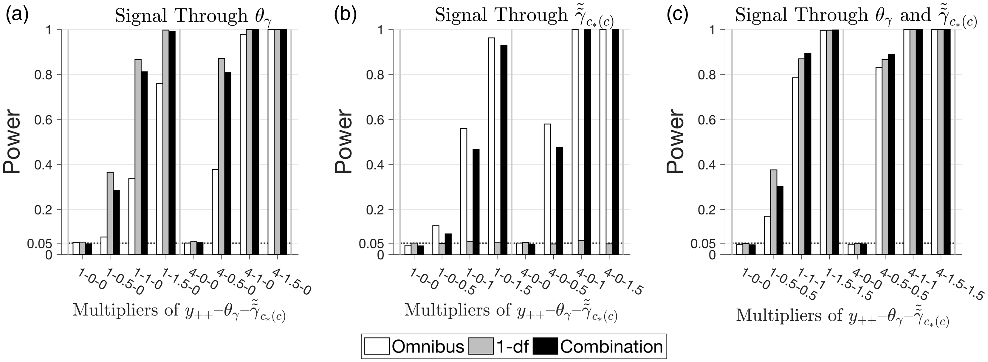

13 Discussion

We developed our new APC model with applications to cancer surveillance research in mind. Our methods are equally appropriate for many other health-related events. For example, using APC analysis, Shiels et al. ¹⁷ analyzed all-cause premature mortality in the US, and Best et al. ¹⁸ analyzed premature mortality from cancer, heart disease, accidents, suicide, and chronic liver disease/cirrhosis.

Our new APC model partitions age, period, and cohort deviations into orthogonal quadratic components plus higher-order terms. Other investigators have developed spline-based methods which include quadratic terms along with other polynomials.^13,19 These approaches provide appealingly smooth estimable functions, but the regression parameters themselves provide little insight. In contrast, the global curvature parameters ${\theta }_{\alpha },{\theta }_{\pi },\hspace{1em}\text{\hspace{1em}and\hspace{1em}}\hspace{1em}{\theta }_{\gamma }$ associated with our orthogonal quadratic polynomials for age, period, and cohort, respectively, quantify how fast on average the trends in the rates are changing. By including these additional parametric terms, our new APC model provides novel estimable functions and hypothesis tests.

We recently developed a random effects model for simultaneous analysis of multiple sets of rates ascertained from multiple population strata over the same Lexis diagram. ²⁰ In that paper, we also present a quadratic model. A key innovation in this report is we use orthogonal polynomials that are characteristic of the underlying Lexis diagram, and demonstrate the surprisingly large utility of doing so. Going forwards, our random effects methods could use the orthogonal parameterization presented here to investigate the heterogeneity of local drifts and local drift trends (i.e. the quantity $-2{\theta }_{\gamma }$ ) over a potentially large number of strata.

Three theoretical points are worth emphasizing. First, all of the parameters and functions described here are identifiable. This is illustrated for example in Figure 3. Second, our new hypotheses tests are level correct, and can be more powerful than the usual global tests. ²¹ Third, the weighted cohort deviations described here are very useful, notwithstanding that unweighted deviations ${\stackrel{\sim }{\gamma }}_{c_{*}}^H$ have been widely used in the past. ²² As we show (Appendix A.6), the absolute difference between the unweighted deviations ${\stackrel{\sim }{\gamma }}_{c_{*}}^H$ and our weighted deviations ${\stackrel{\sim }{\gamma }}_{c_{*}}$ is a linear function of birth cohort. This result implies that the decompositions in Table 2, which are of great utility in practical applications, do not hold if you substitute ${\stackrel{\sim }{\gamma }}_{c_{*}}^H$ for ${\stackrel{\sim }{\gamma }}_{c_{*}}.$

Our new model opens avenues of future methodological research, including comparative analysis, power calculations, and forecasting. ³ For pairwise comparison of from 2 through around 10 strata (for example, 9-registry SEER analyses), we expect our new model will enable more powerful combination tests of log-parallelism and proportionality. ²³ These methods would complement the random effects models that work best when the number of strata is around 10 or more. ²⁰ Asymptotically, the Wald tests have non-central Chi-square distributions, which permits analytical power calculations.

One of the main limitations of the new model is shared by the old: currently, methods are limited to assess goodness-of-fit. One approach that might prove useful would use a smooth Gaussian process to model any residual departures after fitting the usual age, period, and cohort effects. ²⁴ Another important topic is fitting models that incorporate external information, for example, data on established cancer risk factors or screening.

Because our new APC model subsumes a standard APC model yet provides serious advantages, we propose it be considered a new standard. In particular, we believe the value of estimating ${\theta }_{\gamma }$ , the global curvature for cohort, in cancer studies will become increasingly apparent. Whenever ${\theta }_{\gamma }$ is significantly greater than 0, the trend over time is less favorable in younger versus older persons, which is always a cause for concern. In fact, some cancers do appear to be increasing in younger age groups,^25,26 which supports the potential practical utility of our new model. Every statistic introduced in this paper is implemented in our R package (available at https://dceg.cancer.gov/tools/analysis/apc), and we plan to update our web tool (https://analysistools.nci.nih.gov/apc/).

Footnotes

Declaration of conflicting interests

The author(s) declared no potential conflicts of interest with respect to the research, authorship, and/or publication of this article.

Funding

The author(s) received no financial support for the research, authorship, and/or publication of this article.

Appendix A