Bayesian imputation of time-varying covariates in linear mixed models

Abstract

Studies involving large observational datasets commonly face the challenge of dealing with multiple missing values. The most popular approach to overcome this challenge, multiple imputation using chained equations, however, has been shown to be sub-optimal in complex settings, specifically in settings with longitudinal outcomes, which cannot be easily and adequately included in the imputation models. Bayesian methods avoid this difficulty by specification of a joint distribution and thus offer an alternative. A popular choice for that joint distribution is the multivariate normal distribution. In more complicated settings, as in our two motivating examples that involve time-varying covariates, additional issues require consideration: the endo- or exogeneity of the covariate and its functional relation with the outcome. In such situations, the implied assumptions of standard methods may be violated, resulting in bias. In this work, we extend and study a more flexible, Bayesian alternative to the multivariate normal approach, to better handle complex incomplete longitudinal data. We discuss and compare assumptions of the two Bayesian approaches about the endo- or exogeneity of the covariates and the functional form of the association with the outcome, and illustrate and evaluate consequences of violations of those assumptions using simulation studies and two real data examples.

1 Introduction

Missing values are a common challenge in the analysis of observational data, especially in longitudinal studies.

This work is motivated by two research questions from the Generation R Study, ¹ a large longitudinal cohort study from fetal life onward. Specifically, the questions are: (1) “How is gestational weight associated with maternal blood pressure during pregnancy?”, and (2) “How is gestational weight associated with body mass index of the offspring during the first years of life?”. Due to the observational nature of the study, there is a considerable amount of incomplete data, with the particular challenge that missing values do not only occur in the outcome but also in the baseline and time-varying covariates.

There are several well-established approaches to deal with incomplete data, the most popular being multiple imputation using chained equations (MICE), ² which are readily available in standard statistical software. MICE has been shown to work well in many standard settings but may not be optimal in more complex applications, especially with longitudinal or other multivariate outcomes, which cannot be easily included in the imputation models for incomplete covariates in an appropriate manner. ³ Fully Bayesian approaches provide a useful alternative in such complex settings, due to their ability to jointly model multivariate outcomes and incomplete covariates. The most popular omnibus approach in the Bayesian framework postulates a full multivariate normal distribution. ⁴ Although this approach, as well as other approaches, is targeted towards a broad range of applications, in complex settings such as our two motivating research questions, the nature of the data requires careful consideration of the appropriateness of such standard methods and a more dedicated approach may be necessary. Especially with time-varying covariates, imputation and analysis become more demanding and, in order to obtain valid results, require additional considerations about the association between the time-varying covariates and the outcome. Specifically, endogenous covariates, i.e. covariates that are influenced by the outcome, and covariates that have non-standard functional relations with the outcome, can pose challenges that may or may not be adequately handled by standard methods, which usually assume linear associations and implicitly assume exogeneity of the covariates.

In the present paper, we focus on two approaches in the Bayesian framework to deal with covariates that are missing at random. The first approach is described by Carpenter and Kenward. ⁴ The basic idea is to assume a (latent) normal distribution for each incomplete variable and to connect them in such a way that the joint distribution is multivariate normal, which allows straightforward sampling to impute missing values. This approach is a common strategy to implement multiple imputation in longitudinal settings, where it can be used as the data generating step. The resulting data are then analyzed in a second step with a complete data method, not necessarily Bayesian. While the multivariate normality assumption creates a convenient standardized framework, it thereby also implies linear relations between the variables involved, which may not be the case.

The second approach factorizes the joint distribution of the data into a sequence of conditional distributions, where the first conditional distribution can conveniently be chosen to be the analysis model of interest, allowing simultaneous imputation and analysis within the same procedure. This approach has been described previously for time-constant covariates ³ and we will extend it in the present paper to handle exogenous as well as endogenous time-varying covariates. The specification of separate models for each incomplete covariate requires somewhat more consideration than the specification of a multivariate normal distribution, but makes this approach more flexible as well as capable of handling non-linear relationships. We will elucidate the capabilities and limitations of the two approaches with regards to different functional forms for, as well as endo- or exogeneity of, time-varying covariates and demonstrate how the use of an “off the shelf” approach may be problematic in settings that require a more tailored approach.

The remainder of this paper is structured as follows. We start with introducing the motivating dataset and describe in more detail the two research questions from the Generation R Study. In Section 3 we specify the linear mixed model for time-varying covariates and explore different functional forms as well as the issue of endo- and exogeneity. The two methods of interest are introduced in Section 4, where we will also discuss their implied assumptions about endo- or exogeneity of the covariates and their ability to handle different functional forms. We return to the Generation R data in Section 5, where we demonstrate how the two methods under investigation can be applied. A more formal evaluation of the methods follows in Section 6 where we perform a simulation study. Section 7 concludes this paper with a discussion.

2 Generation R data

The Generation R Study is a population-based prospective cohort study from early fetal life onward, conducted in Rotterdam, the Netherlands. ¹ An important field of research within the Generation R Study is the exploration of how the mother's condition during pregnancy may affect her own health and that of her child. Especially weight gain during gestation is of interest as it is closely related to the development of the fetus, as well as to pregnancy comorbidities, such as gestational hypertension, that may adversely affect both mother and child (e.g. Tielemans et al. ⁵ ). Children's growth and body composition, as for instance measured by BMI, is an important determinant of health throughout childhood and later life. Therefore, current research is concerned with the two questions stated in Section 1, i.e. the associations between maternal weight (gain) during pregnancy with maternal blood pressure during pregnancy as well as with child BMI after birth.

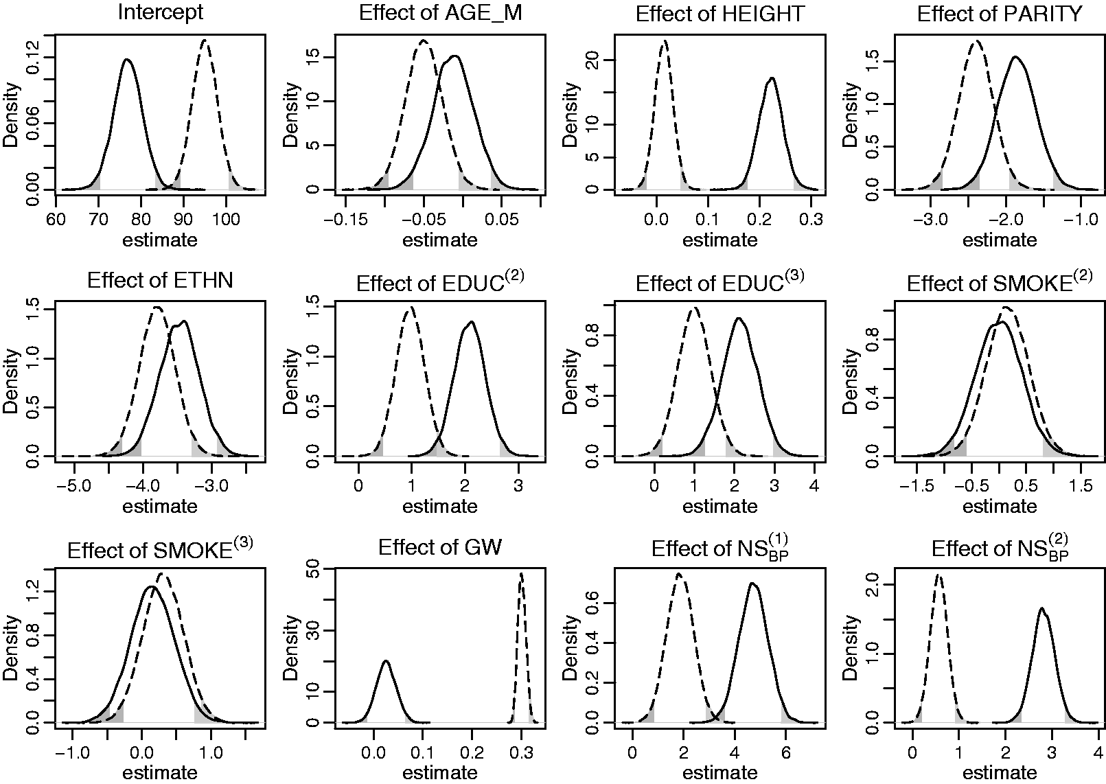
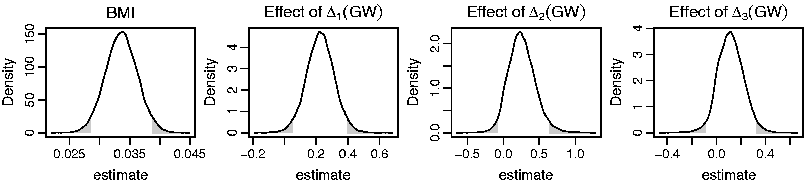
To investigate these two research questions, a subset of variables was extracted from the Generation R Study. The dataset contains information on 7643 mothers who had singleton, live births no earlier than 37 weeks of gestation, and their children. Each woman was asked for her pre-pregnancy weight (baseline) and to visit the research center once in each trimester, during which the weight (gw) was measured and the blood pressure taken. Since women were eligible to enter the study at any gestational age, pre-natal measurements for the first and second trimester are missing for women who enrolled later in pregnancy. Furthermore, there is some intermittent missingness in the gestational and blood pressure data. There were 3515 women for whom all four weight measurements were recorded, 3094 for whom three weight measurements were observed, 859 women had two measurements, and 175 women had only one measurement of weight. The gestational age at each measurement (gage) was recorded and the time point of the baseline measurement was set to be zero for all women. Systolic blood pressure (bp) was measured three times in 4755 women, 2403 women had only two measurements of blood pressure and 477 women just one measurement. For eight women, no blood pressures were recorded. Child BMI was measured up to 12 times between the ages of 2 weeks and 5 years, with a median of seven observations per child; 1848 children had no BMI measurements. The child's age in months (age) was recorded at each BMI measurement and age and sex adjusted standard deviation scores were calculated (bmi). A graphical summary of the missingness pattern of the gestational weight and systolic blood pressure measurements, and the available child BMI measurements are given in Figures 1 to 3 in Appendix B available online. The trajectories of gw, bp and bmi of a random subset of individuals are visualized in Figure 1. Furthermore, we considered a number of potential confounders: maternal age at intake (age_m, continuous, complete), maternal height (height, continuous, 0.38% missing values), parity (parity, binary: nulliparous vs. multiparous, 1.27% missing values), maternal ethnicity (ethn, binary: European vs. other, 5.59% missing values), maternal education (educ, three ordered categories, 9.29% missing values), and maternal smoking habit during pregnancy (smoke, three ordered categories, 12.17% missing values). Maternal BMI (bmi_m) was calculated as gestational weight (kg), measured at time zero, divided by square height (in m).

Figure 1.

Trajectories of maternal weight, maternal systolic blood pressure, and child BMI for a random sample of mothers and children from the Generation R data.

Figure 2.

Posterior distributions of the main regression coefficients in the first application, derived by the sequential approach. The solid (dashed) line represents the endogenous (exogenous) model. The shaded areas mark values outside the 95% credible interval.

Figure 3.

Posterior distributions of a selection of regression coefficients from the second application, derived by the sequential approach. The shaded areas mark values outside the 95% credible interval.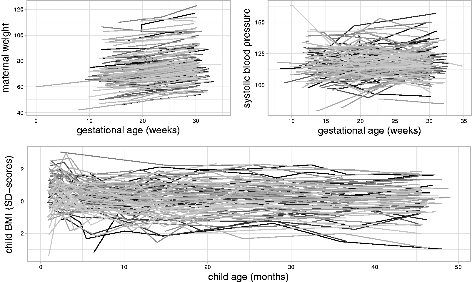

Logistic regression of the complete cases showed that missingness in the baseline covariates (except for parity) was associated with some or all of the other baseline covariates. This indicates that missing values are not completely at random. However, since this study was conducted in the general population, subjects are relatively healthy and the practical settings are such that it is reasonable to believe that missing values in the clinical measurements, as for instance gw or bmi, are at random, given the other variables. It could be argued that missing values in the lifestyle variables, especially in smoke, are not missing at random, because mothers who are smoking might be more inclined not to report it. If this was the case, the mechanism that lead to the missing values had to be included in the imputation procedure since otherwise results would be biased. However, the assumption of randomly missing data is untestable, and the missing data mechanism is usually unknown, necessitating extensive sensitivity analysis. As this exceeds the purpose of this study, we will focus here on randomly missing data. To make the assumption of randomly missing data more plausible, a number of covariates will be considered in the analysis model, since omission of relevant predictor variables may be another reason of not randomly missing data.

3 Modelling longitudinal data with time-varying covariates

3.1 Framework

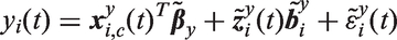
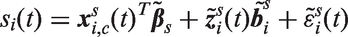
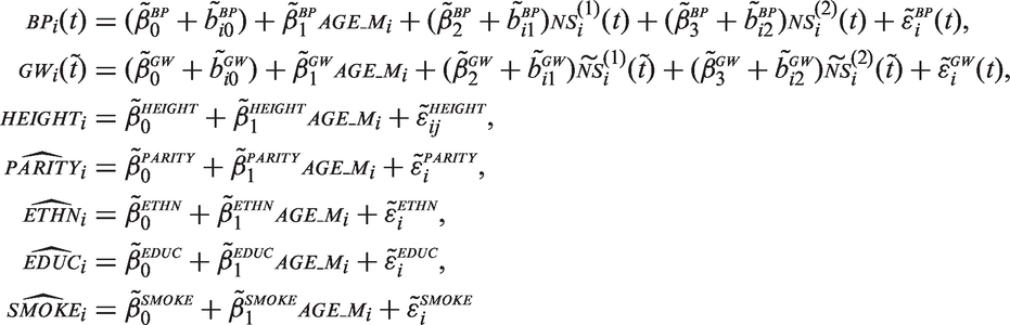
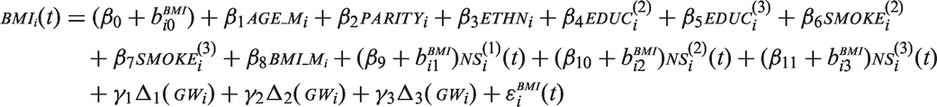
A standard modeling framework for studying the relation between a longitudinal outcome and predictor variables is mixed effects modeling. As in our motivating case studies, often some of these predictors are time-varying. To facilitate exposition and also for notational simplicity, in the following we only consider a single time-varying covariate. In particular, for a continuous longitudinal outcome we postulate the following mixed model

$$y_i(t)=x_i(t{)}^T\beta +f(H_i^s(t),t{)}^T\gamma +z_i(t{)}^T{b}_i+{\varepsilon }_i(t)$$

where $y_i(t)$ is the observation of individual i measured at time t, $\beta$ denotes the vector of regression coefficients of the design matrix of the fixed effects $X_i$ , with $x_i(t)$ being a column vector containing a row of that matrix, $z_i(t)$ , a column vector expressing a row of the design matrix $Z_i$ of the random effects $b_i\sim N(0,D)$ , $\gamma$ is a vector of regression coefficients related to the time-varying covariate $s_i$ , and ${\varepsilon }_i(t)\sim N(0,{\sigma }_y^2)$ is an error term. Except for time itself, $X$ does not contain any time-varying covariates. To include $s$ in the linear predictor of $y$ , assumptions about the relation between the two variables have to be made. These assumptions can be expressed by specifying a function $f(H_i^s(t),t)$ which links the history of the time-varying predictor up to time t, $H_i^s(t)=\{s_i(t_{\mathit{ij}}):0\le t_{\mathit{ij}}\le t,j=1,\dots ,n_i^s\}$ , to the outcome, where t _ij is the time of the j-th measurement of individual i and $n_i^s$ is the number of measurements of $s$ for that individual.

3.2 Functional forms for time-varying covariates

The choice of an appropriate functional form implies that the following two questions need to be addressed. Namely, how are $s_i$ and $y_i$ related with regards to their time scales, and which features of $s_i$ are of interest in the relation with $y_i$ ? The first question asks whether $y_i$ and $s_i$ have been measured in the same time intervals and whether their time scales have the same origin and unit. To allow for settings where $y_i$ and $s_i$ have been measured on different time scales, for instance maternal weight during pregnancy and child BMI after birth, we use t to denote the time scale of $y_i$ and $\tilde{t}$ to denote the time scale of $s_i$ . The second question relates to the specific application and is reflected in the choice of $f(·)$ . Choices that represent relevant features of gestational weight in our two motivating research questions are

$$f(H_i^s(t),t)=s_i(t)$$

(1)

$$f(H_i^s(t),t)=\{{\Delta }_1(s_i),{\Delta }_2(s_i),{\Delta }_3(s_i){\}}^T$$

(2)

with

$${\Delta }_1(s_i)=s_i({\tilde{t}}_1)-s_i({\tilde{t}}_0),$$

$${\Delta }_2(s_i)=s_i({\tilde{t}}_2)-s_i({\tilde{t}}_1),$$

$${\Delta }_3(s_i)=s_i({\tilde{t}}_3)-s_i({\tilde{t}}_2),$$

where (1) represents the commonly chosen linear relation between the value of $s_i$ , e.g. maternal weight, and $y_i$ , e.g. blood pressure, measured at the same time points (i.e. $t=\tilde{t}$ ). Function (2) represents trimester specific weight gain, i.e. the difference of maternal weight over three given time intervals. In a more general notation, (1) could be written as $f(H_i^s(t),t)=s_i(g(t))$ and refer to the value of $s_i$ at a time point that is specified by a function g(t), and (2) could be written as $f(H_i^s(t),t)=s_i(g_2(t))-s_i(g_1(t))$ , where the time intervals are specified by the functions $g_1(t)$ and $g_2(t)$ and may not be the same for all t.

In other applications, it is likely that different functional forms will be more appropriate. Such functions may, for instance, represent cumulative effects or use estimates of random effects associated with the individual profiles of the time-varying covariate. In cases where there is not a specific functional form of interest or there is uncertainty about which functional form is most appropriate, multiple functional forms can be included and shrinkage priors used to reduce correlations between parameters or to select the best suited functional form. ⁶

3.3 Endo- and exogeneity

Another characteristic of the relation between a time-varying covariate and the outcome that needs to be considered is whether the time-varying covariate is exogenous or endogenous. Formally, exogeneity is defined by the following two conditions^7,8

$$\{\begin{array}{l}p(y_i(t),f(H_i^s(t),t)|H_i^y(t^{-}),H_i^s(t^{-}),\theta )=p(y_i(t)|f(H_i^s(t),t),H_i^y(t^{-}),H_i^s(t^{-}),{\theta }_1)\\ \times p(s_i(t)|H_i^y(t^{-}),H_i^s(t^{-}),{\theta }_2)\\ p(s_i(t)|H_i^s(t^{-}),H_i^y(t^{-}),x_i,\theta )=p(s_i(t)|H_i^s(t^{-}),x_i,\theta )\end{array}$$

where $\theta$ is a vector of parameters and other unknown quantities, with ${\theta }^T=({\theta }_1^T,{\theta }_2^T)$ and ${\theta }_1\perp {\theta }_2$ , θ and where $H_i^y(t^{-})$ and $H_i^s(t^{-})$ denote the history of $y$ and $s$ , respectively, up to, but excluding measurements at time t. By specifying the functional relation between $y_i$ and $s_i$ to be a function of the history of $s$ , we avoid dependence of $y_i(t)$ on future values of $s_i$ , which is an additional requirement for exogeneity, see Diggle et al. ⁸ Variables for which these conditions are not satisfied are called endogenous. This may be the case for maternal weight as a predictor variable for blood pressure. Since both variables are measured in the same individual, they may be subject to the same unmeasured influences or causal pathways may be reversed, which often entails endogeneity. In the setting where maternal weight is considered as a predictor of child BMI, however, the assumption of exogeneity may be more likely, since the covariate is measured earlier than the outcome and in different subjects.

Most common methods for inference, like generalized linear (mixed) regression models, assume covariates to be exogenous. If that assumption is wrong and the covariate is in fact endogenous, estimates may be biased.^8,9

4 Bayesian analysis with incomplete covariates

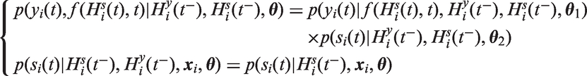
As introduced in Section 2, the motivating questions from the Generation R Study involve outcomes and covariates that are incomplete. This holds for both the baseline and time-varying covariates. Hence, to appropriately investigate the associations of interest, we need to account for missingness. In the Bayesian framework, missing values, whether they are in the outcome or in covariates, can be imputed in a natural and elegant manner. A common assumption, which we make here for the outcome as well as the covariates, is that the missing data mechanism is Missing At Random (MAR), i.e. the probability of a value being unobserved may depend on other observed values but not on values that have not been observed. In addition, the parameters of the analysis model are assumed to be independent of the missingness process. Under these assumptions, the missingness process is ignorable and does not need to be modeled. ¹⁰ Furthermore, this assumption entails that explicit imputation of the outcome is not necessary to obtain valid results and we will therefore focus on settings with incomplete covariates. In this section, we adapt and implement two popular Bayesian approaches for analyzing data with incomplete covariates, namely, the sequential approach,^3,11 and the multivariate normal approach. ⁴ In particular, we extend the first approach to settings with time-varying covariates that may be exogenous or endogenous. Both approaches model the joint distribution of the complete data and draw imputations from the posterior full conditional distributions that result from it, but differ in the way the joint complete data distribution is specified. These differences influence how the two approaches can handle different functional forms as well as exo- vs. endogenous covariates.

We start with some additional notation. As in the motivating data, the time-varying covariate $s$ is assumed incomplete. Missing values in $s$ occur not only due to missed measurements or drop-out but can also be caused when the functional form $f(H_i^s(t),t)$ depends on values of $s$ that have not been (scheduled to be) measured. We use $s_i=(s_{i,\mathit{obs}}^T,s_{i,\mathit{mis}}^T{)}^T$ to distinguish between the observed and missing values of $s$ for individual i. Analogously, we assume two parts for the baseline covariates $X$ on the individual level: $x_{i,\mathit{obs}}$ and $x_{i,\mathit{mis}}$ , which contain the observed and missing values of $x_i$ , respectively. Furthermore, we use the partition $X=(X_c,x_1,\dots ,x_p)$ , where $X_c$ denotes the subset of covariates that are completely observed for all individuals, and $x_1,\dots ,x_p$ are $n\times 1$ vectors of those covariates that contain missing values.

4.1 Sequential approach

The sequential approach to impute missing baseline covariates in models with longitudinal outcomes was previously presented by Erler et al. ³ and will be extended here to incomplete time-varying covariates.

In our setting, the posterior distribution of interest (and associated joint distribution) is

$$\begin{array}{c}p(s_{\mathit{mis}},X_{\mathit{mis}},b,\theta |y,s_{\mathit{obs}},X_{\mathit{obs}})\propto p(y,s_{\mathit{obs}},X_{\mathit{obs}}|s_{\mathit{mis}},X_{\mathit{mis}},b,\theta )\hspace{1em}\hspace{1em}p(s_{\mathit{mis}},X_{\mathit{mis}},b,\theta )\\ =p(y,s_{\mathit{obs}},s_{\mathit{mis}},X_{\mathit{obs}},X_{\mathit{mis}},b,\theta )\end{array}$$

where $\theta$ is a vector of unknown parameters, and can be factorized as

$$p(y|s,X,b,\theta )p(s|X,b,\theta )p(X|\theta )p(b|\theta )p(\theta )$$

(3)

for which all terms can be specified based on known distributions.

The first term in equation (3), i.e. $p(y|s,X,b,\theta )$ , is conveniently chosen to be the analysis model of interest

$$y_i(t)=x_i(t{)}^T{\beta }_{y|s,x}+f(H_i^s(t),t{)}^T\gamma +z_i^y(t{)}^T{b}_i^y+{\varepsilon }_i^y(t)$$

(4)

with random effects $b_i^y\sim N(0,D_y)$ and ${\varepsilon }_i^y(t)\sim N(0,{\sigma }_y^2)$ , and the second factor, representing the imputation model for the time-varying covariate, can be specified analogously as a linear mixed model

$$s_i(\tilde{t})=x_i(\tilde{t}{)}^T{\beta }_{s|x}+z_i^s(\tilde{t}{)}^T{b}_i^s+{\varepsilon }_i^s(\tilde{t})$$

(5)

with $b_i^s\sim N(0,D_s)$ and ${\varepsilon }_i^s(\tilde{t})\sim N(0,{\sigma }_s^2)$ . All variance matrices $D$ and parameters ${\sigma }^2$ are assumed to follow vague inverse Wishart and inverse gamma distributions, respectively. Inclusion of $f(H_i^s(t),t)$ in the linear predictor for $y_i$ allows for a large variety of possibly non-linear relations between $y_i$ and $s_i$ , also when they are measured on different time scales. The joint distribution of the baseline covariates $X$ is often a multivariate distribution of mixed type variables for which usually no closed form solution is known. It can, however, be specified as a sequence of univariate conditional distributions^3,11

$$p(x_1,\dots ,x_p|X_c,{\theta }_x)=p(x_1|X_c,{\theta }_{x_1})\underset{\ell =2}{\overset{p}{\Pi }}p(x_{\ell }|X_c,x_1,\dots ,x_{\ell -1},{\theta }_{x_{\ell }})$$

(6)

with ${\theta }_x^T=({\theta }_{x_1}^T,\dots ,{\theta }_{x_p}^T)$ , where $x_{\ell }$ denotes the ℓ-th incomplete covariate. The univariate conditional distributions are assumed to be members of the exponential family, extended with distributions for ordinal categorical variables, with linear predictors

$$g_{\ell }\{E(x_{\ell }|X_c,x_1,\dots ,x_{\ell -1},{\theta }_{x_{\ell }})\}=X_c{\alpha }_{\ell }+\sum _{q=1}^{\ell -1}{x}_q{\xi }_{{\ell }_q}$$

which allows an easy and flexible specification in settings with many covariates of mixed type, since each link function $g_{\ell }$ can be chosen separately and appropriately for $x_{\ell }$ . Factorizing the joint distribution of the data as in equation (3) has the advantage that the parameters of interest, ${\beta }_{y|s,x}$ , are estimated within each iteration of the imputation procedure, conditional on the current value of the imputed covariates. The simultaneity of imputation and analysis leads to a posterior distribution of the parameters, which automatically takes into account the uncertainty due to the missing values, and no subsequent analysis and pooling, as in the case of multiple imputation approaches, is necessary. Furthermore, the sequential approach differs from MICE in the specification of the imputation models. MICE requires the specification of full-conditional distributions, i.e. to include all other covariates as well as the outcome in the linear predictor of the imputation models, which is not straightforward when the outcome is longitudinal, and may lead to imputation models that are not compatible with the analysis model.^4,12

In the specification described above, the sequential approach implies exogeneity of $s_i$ with regards to the conditions given in Section 3.3, which is demonstrated in Appendix A.1, available online. It can be extended to endogenous time-varying covariates by jointly modeling the random effects from models (4) and (5) as

$$\begin{array}{c}[\begin{array}{c}{b}_i^y\\ b_i^s\end{array}]\sim N(0,[\begin{array}{cc}{D}_y& \hfill D_{\mathit{ys}}\hfill \\ D_{\mathit{ys}}& \hfill D_s\hfill \end{array}]),D_{\mathit{ys}}\ne 0\end{array}$$

When $b_i^y$ and $b_i^s$ are correlated, the joint distribution of the random effects $p(b_i^y,b_i^s)$ is not equal to the product of the marginal distributions $p(b_i^y)$ and $p(b_i^s)$ anymore and the exogeneity conditions are no longer satisfied (for details see Appendix A.2, available online). The sequential approach can be further extended to endogenous baseline covariates by relaxing the assumption of independence between the residuals of the covariate and the analysis model, e.g. by assuming a joint distribution of the residuals and the random effects $b_i^y$ .

4.2 Multivariate normal approach

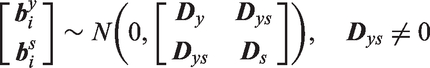
A popular alternative to handle missing covariates is the multivariate normal approach described in detail by Carpenter and Kenward. ⁴ The idea behind this approach is to assume (latent) normal distributions for all incomplete variables and the outcome, and to connect them in such a way that the resulting joint distribution is multivariate normal, which eases the sampling of imputed values. Specification of the joint distribution of the data is, hence, not based on a sequence but on a chosen multivariate distribution of known type. In our setting, the posterior distribution of interest can be written and factorized as

$$\begin{array}{c}p(s_{\mathit{mis}},X_{\mathit{mis}},\tilde{b},\tilde{\theta }|y,s_{\mathit{obs}},X_{\mathit{obs}})\propto p(y,s,X_{\mathit{mis}},X_{\mathit{obs}},\tilde{b},\tilde{\theta })=p(y,s,X_c,x_1,\dots ,x_p,\tilde{b},\tilde{\theta })\\ =p(y,s,x_1,\dots ,x_p|X_c,\tilde{b},\tilde{\theta })p(\tilde{b}|\tilde{\theta })p(\tilde{\theta })\end{array}$$

(7)

where the first factor on the right side of equation (7) is assumed to be a multivariate normal distribution, $\tilde{b}$ is a random effect that is associated with $y$ and $s$ , and $\tilde{\theta }$ is a vector of parameters. The multivariate normal distribution can be constructed by specifying linear (mixed) models for the outcome and incomplete covariates, i.e. the time-varying and incomplete baseline covariates

$$y_i(t)=x_{i,c}^y(t{)}^T{\tilde{\beta }}_y+{\tilde{z}}_i^y(t){\tilde{b}}_i^y+{\tilde{\varepsilon }}_i^y(t)$$

$$s_i(t)=x_{i,c}^s(t{)}^T{\tilde{\beta }}_s+{\tilde{z}}_i^s(t){\tilde{b}}_i^s+{\tilde{\varepsilon }}_i^s(t)$$

$${\widehat{x}}_{i,\ell }=x_{i,c}^x{\hspace{0.17em}}^T{\tilde{\beta }}_{x,\ell }+{\tilde{\epsilon }}_{i,\ell }^x,\ell =1,\dots ,p,$$

where $x_{i,c}^y(t),x_{i,c}^s(t)$ and $x_{i,c}^x$ are rows of the matrices $X_c^y$ , $X_c^s$ and $X_c^x$ which are (possibly different) subsets of $X_c,{\hat{x}}_{i,\ell }$ denotes the value from a (latent) normal distribution that corresponds to the missing value of the ℓ-th incomplete covariate for individual i, ${\tilde{\beta }}_y,{\tilde{\beta }}_s$ and ${\tilde{\beta }}_x=({\tilde{\beta }}_{x_1}^T,\dots ,{\tilde{\beta }}_{x_p}^T{)}^T$ are regression coefficients, ${\tilde{z}}_i^y(t)$ and ${\tilde{z}}_i^s(t)$ are rows of the design matrices ${\tilde{Z}}_i^y$ and ${\tilde{Z}}_i^s$ of the random effects ${\tilde{b}}_i^y$ and ${\tilde{b}}_i^s$ . Note that the models specified here are different from the ones in the sequential approach, since here the predictors only contain the completely observed covariates $X_c$ . The parameters $\tilde{\beta }$ are not the same as the parameters ${\beta }_{y|s,x}$ , used in the sequential approach. To obtain estimates of ${\beta }_{y|s,x}$ that take into account the uncertainty due to the missing values, multiple imputation may be performed. This involves repeating the imputation a number of times to create multiple imputed datasets, which can then be analyzed with appropriate Bayesian or non-Bayesian methods. Pooled estimates from frequentist analyses can be calculated using Rubin's Rules. ¹³ Although imputation with the multivariate normal approach is valid for endogenous covariates, this may not be the case for many standard analysis methods that imply exogeneity of the covariates, which may pose an additional challenge.

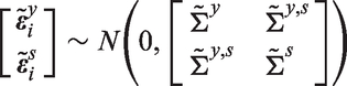
To produce the multivariate normal distribution, the models specified above are then connected through their random effects and error terms which are assumed to have a joint multivariate normal distribution

$$\left[\begin{array}{c}{\tilde{b}}_i^y\\ {\tilde{b}}_i^s\\ {\tilde{\epsilon }}_i^x\end{array}\right]\sim N\left(0,\left[\begin{array}{lll}{\tilde{\text{D}}}_y\hfill & {\tilde{\text{D}}}_{y,s}\hfill & \text{cov}({\tilde{b}}_i^y,{\tilde{\epsilon }}_i^x)\hfill \\ {\tilde{\text{D}}}_{y,s}\hfill & {\tilde{\text{D}}}_s\hfill & \text{cov}({\tilde{b}}_i^s,{\tilde{\epsilon }}_i^x)\hfill \\ \text{cov}({\tilde{b}}_i^y,{\tilde{\epsilon }}_i^x)\hfill & \text{cov}({\tilde{b}}_i^s,{\tilde{\epsilon }}_i^x)\hfill & {\tilde{\Sigma }}^x\hfill \end{array}\right]\right)$$

where ${\tilde{D}}_y$ and ${\tilde{D}}_s$ denote the covariance matrices of the random effects ${\tilde{b}}_i^y$ and ${\tilde{b}}_i^s$ , respectively, ${\tilde{D}}_{y,s}$ is a matrix containing parameters that describe the covariance between the two sets of random effects, and ${\tilde{\Sigma }}^x$ is the, usually diagonal, covariance matrix of the error terms ${\tilde{\varepsilon }}_i^x=({\tilde{\varepsilon }}_{i,1}^x,\dots ,{\tilde{\varepsilon }}_{i,p}^x{)}^T$ .

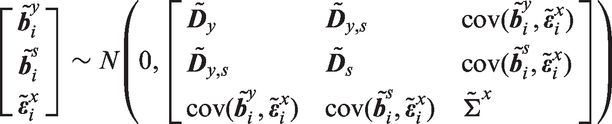
The error terms of the two longitudinal variables are assumed to be normally distributed as well, and may be modeled jointly as

$$\left[\begin{array}{c}{\tilde{\epsilon }}_i^y\\ {\tilde{\epsilon }}_i^s\end{array}\right]\sim N\left(0,\left[\begin{array}{ll}{\tilde{\Sigma }}^y\hfill & {\tilde{\Sigma }}^{y,s}\hfill \\ {\tilde{\Sigma }}^{y,s}\hfill & {\tilde{\Sigma }}^s\hfill \end{array}\right]\right)$$

where ${\tilde{\Sigma }}^y$ and ${\tilde{\Sigma }}^s$ denote the covariance matrices of ${\tilde{\varepsilon }}_i^y$ and ${\tilde{\varepsilon }}_i^s$ , respectively, and ${\tilde{\Sigma }}^{y,s}$ is a matrix describing the covariance between the error terms of $y_i$ and the error terms of $s_i$ . Allowing the error terms of the longitudinal variables to be correlated allows for more flexibility. Which covariance structure is appropriate, however, depends on the unknown functional relation between $y$ and $s$ .

The latent normal model for a binary or ordinal covariate $x_{\mathit{mi}{s}_{\ell }}$ with K categories can be written as

$$\begin{array}{cc}\begin{array}{l}{\widehat{x}}_{i,mi{s}_{\ell }}\le {\kappa }_1\\ {\widehat{x}}_{i,mi{s}_{\ell }}\in ({\kappa }_{k-1},{\kappa }_k]\\ {\widehat{x}}_{i,mi{s}_{\ell }}>{\kappa }_{K-1}\end{array}& \begin{array}{l}\text{if\hspace{0.17em}\hspace{0.17em}}{x}_{i,mi{s}_{\ell }}=1,\\ \text{if\hspace{0.17em}\hspace{0.17em}}{x}_{i,mi{s}_{\ell }}=k,k\in (2,\dots ,K-1),\\ \text{if\hspace{0.17em}\hspace{0.17em}}{x}_{i,mi{s}_{\ell }}=k\end{array}\end{array}$$

To keep the model identified, the variance of ${\hat{x}}_{i,\mathit{mi}{s}_{\ell }}$ has to be fixed, e.g., to one, which complicates sampling of ${\tilde{\Sigma }}^x$ . For continuous covariates ${\hat{x}}_{i,\mathit{mi}{s}_{\ell }}=x_{i,\mathit{mi}{s}_{\ell }}$ and no restriction of the variance is necessary.

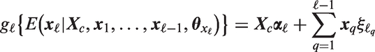
As in the sequential approach, the use of variable specific random effects design matrices ${\tilde{Z}}_i^y$ and ${\tilde{Z}}_i^s$ enables this approach to handle time-varying covariates that are measured on a different time scale than the outcome. The connection of the imputation models by joint random effects and/or error terms, however, implies a linear relation between the variables. When the relation between $y_i$ and $s_i$ is non-linear, the true joint distribution is not multivariate normal and does not generally have a closed form. ⁴ The multivariate normal approach may, hence, be less suitable for applications with non-linear relations.

Since $b_i^y$ and $b_i^s$ are modeled jointly and assumed to be correlated, the conditions for exogeneity are violated, which can be shown using similar arguments as provided in Appendix A.2, available online for the sequential approach with correlated random effects. The multivariate normal approach thus implies endogeneity of $s_i$ .

5 Analysis of the Generation R data

We now return to the Generation R data introduced in Section 2 and demonstrate how to use the two methods discussed above to investigate the two motivating research questions. As indicated earlier, the first question enables the investigation of the impact of mis-specifying the exo-/endogeneity assumption, while the second question requires the use of a non-standard functional form.

5.1 Association between blood pressure and gestational weight

Gestational hypertension is a known risk factor for various health outcomes in mothers as well as their children. One potentially influential factor for this condition is gestational weight, which will be investigated here. Whilst there are several papers exploring the relationship of gestational weight gain and the development of hypertensive conditions during pregnancy, the exact nature and functional form of the relation between these variables have yet to be explored in detail. Given the information available and the characteristics of the dataset at hand, a reasonable choice of functional form is to assume a linear relation between gestational weight (gw) and systolic blood pressure (bp) at the same time points, i.e. $f(H_i^{\mathit{GW}}(t),t)={\mathit{GW}}_i(t)$ . Furthermore, the relation between these two variables is likely influenced by many unmeasured factors, which makes the standard assumption of exogeneity for gestational weight questionable. To investigate how much the estimates may be influenced by the assumption of exo- or endogeneity in practice, we performed the analysis twice, once under the assumption that gestational weight was endogenous, and once under the common default assumption of exogeneity, and compared the results.

Since both longitudinal variables in this application have non-linear evolutions over time, we modeled their trajectories using natural cubic splines with two degrees of freedom (df) for the effect of gestational age, in the formulas below represented by $N{S}_i^{(1)}(t),N{S}_i^{(2)}(t)$ , and ${\widetilde{\mathit{NS}}}_i^{(1)}(\tilde{t}),{\widetilde{\mathit{NS}}}_i^{(2)}(\tilde{t})$ , respectively. Taking into account a number of potential confounding covariates (see Section 2), the model of interest in this application can be written as

$$\begin{array}{c}B{P}_i(t)=({\beta }_0+b_{i0}^{BP})+{\beta }_{1}AGE\_M_i+{\beta }_{2}HEIGH{T}_i+{\beta }_{3}PARIT{Y}_i+{\beta }_{4}ETH{N}_i+{\beta }_{5}EDU{C}_i^{(2)}+{\beta }_{6}EDU{C}_i^{(3)}\\ +{\beta }_{7}SMOK{E}_i^{(2)}+{\beta }_{8}SMOK{E}_i^{(3)}+({\beta }_9+b_{i1}^{BP})N{S}_i^{(1)}(t)+({\beta }_{10}+b_{i2}^{BP})N{S}_i^{(2)}(t)+\gamma G{W}_i(t)+{\epsilon }_i^{BP}(t).\end{array}$$

In the sequential approach, we used a linear mixed model to impute missing values of gw, specifically

$$\begin{array}{l}G{W}_i(\tilde{t})=({\alpha }_0+b_{i0}^{GW})+{\alpha }_{1}AGE\_M_i+{\alpha }_{2}HEIGH{T}_i+{\alpha }_{3}PARIT{Y}_i+{\alpha }_{4}ETH{N}_i+{\alpha }_{5}EDU{C}_i^{(2)}+{\alpha }_{6}EDU{C}_i^{(3)}+{\alpha }_{7}SMOK{E}_i^{(2)}\\ +{\alpha }_{8}SMOK{E}_i^{(3)}+({\alpha }_9+b_{i1}^{GW}){\widetilde{NS}}_i^{(1)}(\tilde{t})+({\alpha }_{10}+b_{i2}^{GW}){\widetilde{NS}}_i^{(2)}(\tilde{t})+{\epsilon }_i^{GW}(\tilde{t})\end{array}$$

and specified the conditional distributions for the missing covariates from equation (6) as linear, logistic and cumulative logistic regression models. The random effects of the models for gw and bp were modeled jointly as ${(b_{i0}^{\mathit{BP}},b_{i1}^{\mathit{BP}},b_{i2}^{\mathit{BP}},b_{i0}^{\mathit{GW}},b_{i1}^{\mathit{GW}},b_{i2}^{\mathit{GW}})}^T\sim N(0,\text{D})$ in the endogenous setting and independently as ${(b_{i0}^{BP},b_{i1}^{BP},b_{i2}^{BP},)}^T\sim N(0,{\text{D}}_{BP})$ and ${(b_{i0}^{\mathit{GW}},b_{i1}^{\mathit{GW}},b_{i2}^{\mathit{GW}})}^T\sim N(0,{\text{D}}_{\mathit{GW}})$ in the exogenous setting. Vague priors were used for all parameters. Following the advice of Garrett et al., ¹⁴ we assumed independent normal distributions with mean zero and variance 9/4 for regression coefficients in categorical models (logistic and cumulative logistic) since that choice leads to a prior distribution for the outcome probabilities that is relatively flat between zero and one. All continuous covariates were scaled to have mean zero and standard deviation one, for computational reasons, and the posterior estimates were transformed back to be interpretable on the original scale of the variables. The endogenous as well as the exogenous setting was implemented using R ¹⁵ and JAGS. ¹⁶ Convergence of the posterior chains was checked using the Gelman–Rubin criterion. ¹⁷ The posterior estimates were considered precise enough if the Monte Carlo error was less than five percent of the parameter's standard deviation. ¹⁸ In the endogenous setting, only 5000 iterations (in each of three posterior chains) were necessary, while in the exogenous setting 20,000 iterations were required to satisfy this criterion. Posterior predictive checks were used to evaluate if the assumed model fitted the data appropriately.

In the multivariate normal approach, the imputation models can be specified as

$$\begin{array}{l}B{P}_i(t)=({\tilde{\beta }}_0^{BP}+{\tilde{b}}_{i0}^{BP})+{\tilde{\beta }}_1^{BP}AGE\_M_i+({\tilde{\beta }}_2^{BP}+{\tilde{b}}_{i1}^{BP})N{S}_i^{(1)}(t)+({\tilde{\beta }}_3^{BP}+{\tilde{b}}_{i2}^{BP})N{S}_i^{(2)}(t)+{\tilde{\epsilon }}_i^{BP}(t),\\ G{W}_i(\tilde{t})=({\tilde{\beta }}_0^{GW}+{\tilde{b}}_{i0}^{GW})+{\tilde{\beta }}_1^{GW}AGE\_M_i+({\tilde{\beta }}_2^{GW}+{\tilde{b}}_{i1}^{GW}){\widetilde{NS}}_i^{(1)}(\tilde{t})+({\tilde{\beta }}_3^{GW}+{\tilde{b}}_{i2}^{GW}){\widetilde{NS}}_i^{(2)}(\tilde{t})+{\tilde{\epsilon }}_i^{GW}(t),\\ HEIGH{T}_i={\tilde{\beta }}_0^{HEIGHT}+{\tilde{\beta }}_1^{HEIGHT}AGE\_M_i+{\tilde{\epsilon }}_{ij}^{HEIGHT},\\ {\widehat{PARITY}}_i={\tilde{\beta }}_0^{PARITY}+{\tilde{\beta }}_1^{PARITY}AGE\_M_i+{\tilde{\epsilon }}_i^{PARITY},\\ {\widehat{ETHN}}_i={\tilde{\beta }}_0^{ETHN}+{\tilde{\beta }}_1^{ETHN}AGE\_M_i+{\tilde{\epsilon }}_i^{ETHN},\\ {\widehat{EDUC}}_i={\tilde{\beta }}_0^{EDUC}+{\tilde{\beta }}_1^{EDUC}AGE\_M_i+{\tilde{\epsilon }}_i^{EDUC},\\ {\widehat{SMOKE}}_i={\tilde{\beta }}_0^{SMOKE}+{\tilde{\beta }}_1^{SMOKE}AGE\_M_i+{\tilde{\epsilon }}_i^{SMOKE}\end{array}$$

and their random effects and error terms modeled jointly as

$${({\tilde{b}}_{i0}^{\mathit{BP}},{\tilde{b}}_{i1}^{\mathit{BP}},{\tilde{b}}_{i2}^{\mathit{BP}},{\tilde{b}}_{i0}^{\mathit{GW}},{\tilde{b}}_{i1}^{\mathit{GW}},{\tilde{b}}_{i2}^{\mathit{GW}},{\tilde{\epsilon }}_i^{\mathit{HEIGHT}},{\tilde{\epsilon }}_i^{\mathit{PARITY}},{\tilde{\epsilon }}_i^{\mathit{ETHN}},{\tilde{\epsilon }}_i^{\mathit{EDUC}},{\tilde{\epsilon }}_i^{\mathit{SMOKE}})}^T\sim N(0,\tilde{\text{D}})$$

where the diagonal elements that correspond to parity, ethn, educ and smoke are fixed to 1, and ${\left\{{\tilde{\epsilon }}_i^{BP}(t),{\tilde{\epsilon }}_i^{GW}(t)\right\}}^T\sim N(0,\tilde{\mathbf{\Sigma }}(t))$ .

Using current versions of the software packages JAGS or WinBUGS ¹⁹ it is not possible to sample from such a restricted covariance matrix and we will, therefore, only present results from the sequential approach for the Generation R applications. These results are presented in Figure 2. The solid line represents the posterior distribution of the regression coefficients obtained by the sequential approach under the assumption that gw was endogenous, while the dashed line depicts the corresponding posterior distributions when gw was assumed to be exogenous. The shaded areas in the tails of the distributions mark values outside the 95% credible interval (CI). It can easily be seen that the assumption of exo- or endogeneity has great impact on the posterior distribution. Especially the posterior distribution of the effect of the time-varying covariate, gw, differs substantially between the two models. While in the endogenous model the posterior mean of this effect was 0.03 with a 95% CI that includes zero [−0.01, 0.07], this estimate was 0.30 [0.29, 0.32], when gw was assumed to be exogenous. Also in other parameters, such as the regression coefficients for height, educ and the non-linear effect of gage, the posterior distributions differed considerably.

A possible explanation for these differences is that in the exogenous model the correlation between gw and bp is only captured in the parameter γ whereas in the endogenous model it is split between γ and the covariance between the random effects of the model for bp and gw, i.e. the elements in the upper right quadrant of $D$ . Figure 4 in Appendix B, available online shows the posterior density of the elements of the matrix $D$ . Most of the parameters describing the covariance between $b^{\mathit{GW}}$ and $b^{\mathit{BP}}$ estimate the respective covariance to be different from zero. The exogenous model implies that these parameters are zero and does not estimate them. Interpreting the results from the endogenous model, we may conclude that gw and bp are correlated, but that there is no evidence that changes in gw cause changes in bp.

5.2 Association between gestational weight gain and child BMI

Fetal development follows a well researched course which is influenced by maternal health throughout pregnancy. Specifically the effect of gestational weight gain may vary between different periods of pregnancy, i.e. different periods of fetal development. Hence, the effect of trimester-specific weight gain is often a predictor of interest. How much weight gain is considered healthy varies with maternal BMI before pregnancy (bmi_m) which, therefore, needs to be considered as predictor variable in this research question. Since gw is observed entirely prior to the outcome (bmi), it might not be considered to be a time-varying covariate in the narrow sense, i.e. it does not change throughout the time range of the outcome measurements. Nevertheless, it does change over time and an appropriate characterization of this change is essential to obtain results that allow meaningful conclusions with regards to the research question at hand.

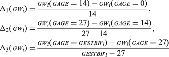
We calculated trimester-specific weight gain as the differences between weight before pregnancy, 14 weeks of gestation, 27 weeks of gestation and at (or right before) birth (gestbir), and scaled these differences to reflect weight gain per week. The functional relation between gw and bmi can thus be represented as

$$f(H_i^{GW}(t),t)={\left\{{\Delta }_1(G{W}_i),{\Delta }_2(G{W}_i),{\Delta }_3(G{W}_i)\right\}}^T,$$

with

$$\begin{array}{l}{\Delta }_1(G{W}_i)=\frac{G{W}_i(GAGE=14)-G{W}_i(GAGE=0)}{14},\\ {\Delta }_2(G{W}_i)=\frac{G{W}_i(GAGE=27)-G{W}_i(GAGE=14)}{27-14},\\ {\Delta }_3(G{W}_i)=\frac{G{W}_i(GAGE={\mathit{GESTBIr}}_i)-G{W}_i(GAGE=27)}{{\mathit{GESTBIr}}_i-27}\end{array}$$

As in the first application, we assumed a non-linear evolution of gw over time, which was modeled using a natural cubic spline for gage with 2 df. Also, the trajectories of child BMI, for which age and gender specific standard deviation scores (SDS) were used, were non-linear and therefore modeled using a natural cubic spline with 3 df for age, in the formula below represented by $N{S}_i^{(1)}(t),N{S}_i^{(2)}(t)$ and $N{S}_i^{(1)}(t),N{S}_i^{(3)}(t)$ . Since gw was measured before birth and bmi only after birth, we assumed that gw was exogenous in this application.

The analysis model for this research question can be written as

$$\begin{array}{c}BM{I}_i(t)=({\beta }_0+b_{i0}^{BMI})+{\beta }_{1}AGE\_M_i+{\beta }_{2}PARIT{Y}_i+{\beta }_{3}ETH{N}_i+{\beta }_{4}EDU{C}_i^{(2)}+{\beta }_{5}EDU{C}_i^{(3)}+{\beta }_{6}SMOK{E}_i^{(2)}\\ +{\beta }_{7}SMOK{E}_i^{(3)}+{\beta }_{8}BMI\_M_i+({\beta }_9+b_{i1}^{BMI})N{S}_i^{(1)}(t)+({\beta }_{10}+b_{i2}^{BMI})N{S}_i^{(2)}(t)+({\beta }_{11}+b_{i3}^{BMI})N{S}_i^{(3)}(t)\\ +{\gamma }_1{\Delta }_1(G{W}_i)+{\gamma }_2{\Delta }_2(G{W}_i)+{\gamma }_3{\Delta }_3(G{W}_i)+{\epsilon }_i^{BMI}(t)\end{array}$$

The analysis was again performed using the sequential approach, where imputation models for gw and the baseline covariates were specified analogous to the first application. To reduce correlation between the elements of $\gamma$ , an elastic net shrinkage hyper-prior for the variance parameters of $\gamma$ was used. ²⁰

Results from the analysis of this second research question are presented in Figure 3. Only the posterior distributions of the parameters relating to bmi_m and gw are shown as these are the parameters of interest here. It can be seen that children of mothers with higher baseline BMI had higher BMIs as well – an increase of one kg/m² resulted on average in a 0.03 SDS higher child BMI (95% CI [0.03, 0.04]). Higher gestational weight gain during the first trimester was associated with higher child BMI (0.23 SDS increase per kg weekly weight gain; 95% CI [0.05, 0.40]). Even though the posterior mean of the effect of weekly gestational weight gain during the second trimester was slightly higher (0.26), due to the increased uncertainty of this estimate (95% CI [−0.08, 0.65]), there was no evidence of an association with the trajectories of child BMI. There was also no evidence that weight gain during the last trimester was a relevant predictor of child BMI (0.12; 95% CI [−0.09, 0.33]).

6 Simulation study

To evaluate the performance of the two imputation approaches described in Section 4 with regards to mis-specification of the endo- or exogeneity of a time-varying covariate and the bias introduced by mis-specification of the functional form in a more controlled setting, we performed a simulation study in which we compared results from correctly specified models with those that are mis-specified, for data generated in a range of different scenarios and different missing mechanisms. Specifically, the key objectives were

to confirm that both approaches provide unbiased estimates when the models are correctly specified during imputation and analysis,

to investigate how mis-specification of the endo- or exogeneity influences the results, and

to explore bias due to mis-specification of the functional form, specifically

the bias introduced during imputation due to the implied linearity assumption of the multivariate normal approach when the true functional form is non-linear, and

the bias introduced when the imputation model as well as the analysis model are mis-specified as linear.

6.1 Design

We simulated 200 datasets in each of six scenarios that differed in the endo-/exogeneity of the covariate, the functional form and the model (sequential or multivariate normal) that was used. Common to all scenarios was that 10 repeated measurements of a normally distributed time-varying covariate and a conditionally normal outcome variable, with measurements at the same, unbalanced time points, were created. Under the sequential approach, data were generated with a linear or a quadratic relation between covariate and outcome, where the covariate was either exogenous or endogenous. For the multivariate normal model (which always generates data with a linear relation between the outcome and an endogenous covariate), we considered two scenarios with regards to the correlation of the error terms, where in one scenario the error terms of outcome and covariate were independent and in the other correlated.

Missing values were created in the time-varying covariate according to two MAR mechanisms, in which the probability of the time-varying covariate being missing either only depended on the outcome at the same time point or on the outcome at the same time point as well as the covariate at the previous time point.

Details on the exact setup of the simulation study are given in Appendix C.1, available online.

6.2 Analysis models

Each of the datasets was analyzed using both approaches with different assumptions regarding the endo- or exogeneity of the covariate and the functional form, before values were deleted, and for both missing mechanisms. The complete dataset was analyzed using function lmer() from the R-package lme4^15,21 as well as with the sequential approach. Missing data were imputed and analyzed with the sequential approach, where the random effects were modeled according to the current assumption of exo- or endogeneity, and the imputation was repeated twice with the multivariate normal approach (once using the model with independent error terms and once assuming correlated error terms). Each time, 10 imputed datasets were created by drawing values from the posterior chains of the incomplete covariate and analyzed analogous to the analysis of the complete data. When the covariate was assumed exogenous, lmer() was used and the coefficients from the 10 corresponding analyses pooled using Rubin's Rules. ¹³ When the covariate was assumed to be endogenous, the sequential approach with correlated random effects was used and the 10 sets of posterior MCMC chains combined to calculate posterior summary measures.

An overview of the assumptions and models used can be found in Table 2 in Appendix C.2, available online. The specific parameter values that were used are given in Tables 3 and 4 in Appendix C.3, available online.

6.3 Results

First, we found that the sequential approach provided unbiased estimates, when comparing the results from the analysis of the complete data to the true parameters that were used to generate the data. Second, in all scenarios, results were very similar for both MAR mechanisms and we will, hence, not distinguish them during the further description of the results.

Regarding our first objective, the comparison of the sequential and the multivariate normal approach when exo- or endogeneity and functional form were specified correctly, we found that both approaches were unbiased and their 95% credible intervals had the desired coverage. However, mis-specification of the error terms in the multivariate normal approach as independent had the overall largest impact on the results (estimates were on average half the value of the estimate from the analysis of the complete data and CIs had 0% coverage). Based on this finding, we excluded the multivariate normal approach with independent error terms from further comparisons. Moreover, we saw that mis-specification of an endogenous covariate as exogenous resulted in bias while mis-specification of an exogenous covariate as endogenous did not. This was the case for both approaches, and linear as well as quadratic (only for the sequential approach) functional form. With respect to our third objective, the simulation study showed that imputation with the multivariate normal approach (with correlated error terms) in a setting where the functional form was correctly assumed to be quadratic during the subsequent analysis had the second largest impact, with a relative bias of approximately 0.8, and resulted in CIs with coverage of close to 0%. The bias that was added due to mis-specification of the functional form as linear during imputation as well as analysis, as compared to the results from the analysis of the complete data under the same mis-specification, was small and overall comparable between the multivariate normal and the sequential approach. These findings were the same irrespective of the exo- or endogeneity of the covariate. Plots of the results from the simulation study as well as a detailed discussion of these results can be found in Appendix C.4, available online.

In summary, the results of this simulation study demonstrate the impact that imprudent acceptance of default assumptions, like exogeneity, linear relations between variables, or (conditioned on random effects) uncorrelated error terms may have. Plots of the results from the simulation study as well as a detailed discussion of these results can be found in Appendix C.4, available online.

7 Discussion

Motivated by two research questions from the Generation R study, we investigated two Bayesian approaches to handle missing covariate data in models with longitudinal outcomes and time-varying covariates. Specifically, we compared the multivariate normal approach, a widely known omnibus approach, to the more custom-designed sequential approach, which we extended to handle endogenous time-varying covariates. The focus of this comparison was on the ability to take into account different functional relations between such covariates and the outcome, and the suitability for exogenous as well as endogenous covariates.

The analysis of our real data applications illustrated the necessity for methods that allow for complex functional relations and endogenous covariates. Simulation studies confirmed that in our setting, methods that make the common assumption of exogeneity of a time-varying covariate provide biased estimates. The assumption of endogeneity during imputation and analysis, however, did not introduce any bias, which suggests to choose the endogenous specification, e.g., to model the random effects of the outcome and the time-varying covariate correlated, as a default. The simulation study also demonstrated that imputation with the multivariate normal approach in settings where the implied assumption of linear associations between variables is violated can be biased. Furthermore, great care should be taken when assumptions about the correlation structure of the error terms is made in the multivariate normal approach, as mis-specification may result in large bias. Results indicated that the sequential approach is more robust with regards to this type of mis-specification; however, future research is required to evaluate this further. Overall, the sequential approach performed well and proved to be a suitable method to impute and analyze longitudinal data with possibly endogenous time-varying covariates.

The ability of the sequential approach to handle various functional forms, and to provide estimates in settings with endogenous time-varying covariates, can be seen as its biggest advantages. Moreover, it can handle non-linear associations of baseline covariates and interaction terms involving incomplete covariates without the need of approximations like the ‘just another variable’ approach or passive imputation via transformation.^12,22,23 Even in settings where there is no single functional form of interest, but several candidate functions, it may be applied in combination with shrinkage techniques which may help the decision which functional form is most appropriate.

In the present paper, we focused on a single time-varying covariate and ignorable missing data mechanisms; however, extensions of the sequential approach to accommodate more complex settings are possible. Multiple time-varying covariates can be added to the linear predictor of the analysis model. Imputation models for the time-varying covariates could either be specified assuming independence between different time-varying covariates, i.e. excluding them from each other's linear predictor, assuming joint multivariate distributions for their random effects and/or error terms, or by specifying a functional form of one time-varying covariate to be included in the linear predictor of another covariate, analogous to the specification of the analysis model described in Section 3. The second option may be a convenient choice if a linear relation between the time-varying covariates is a reasonable assumption. When the missing data mechanism is non-ignorable, this can be taken into account by extending the specification of the joint distribution with terms that either describe the selection mechanism (i.e. the missingness pattern given the data) or specify how the distribution of the data depends on the missingness pattern.^2,4,9

A reason why the multivariate normal approach may be preferred in practice is its availability in software packages, as, for instance, the R-package jomo ²⁴ or REALCOM-impute. ²⁵ Those implementations also provide samplers that can handle restricted covariance matrices. More tailored approaches, like the sequential approach, usually need to be implemented by hand, which, however, can be done in existing Bayesian software packages such as JAGS or WinBUGS in a straightforward way. In Appendix C.5, available online, we give example syntax for both approaches. This syntax can easily be extended to include complete or incomplete baseline covariates (see also the Appendix of Erler et al. ³ ). Additional example syntax can be provided upon request.

When imputing and analyzing complex datasets, researchers need to deliberate if standard methods that are easy to apply meet the requirements of the application at hand, specifically, if the assumptions of those methods are met. It is our opinion that too often this is not the case and standard approaches are applied even when they are not adequate. Therefore, we plead for the use of methods that are flexible enough to be adapted to the specific characteristics of a problem. In the context of imputation and analysis of longitudinal data with possibly endogenous time-varying covariates, the sequential approach presented in this paper is such an approach.