Two-part models with stochastic processes for modelling longitudinal semicontinuous data: Computationally efficient inference and modelling the overall marginal mean
Open accessResearch articleFirst published online December, 2018
Two-part models with stochastic processes for modelling longitudinal semicontinuous data: Computationally efficient inference and modelling the overall marginal mean
Several researchers have described two-part models with patient-specific stochastic processes for analysing longitudinal semicontinuous data. In theory, such models can offer greater flexibility than the standard two-part model with patient-specific random effects. However, in practice, the high dimensional integrations involved in the marginal likelihood (i.e. integrated over the stochastic processes) significantly complicates model fitting. Thus, non-standard computationally intensive procedures based on simulating the marginal likelihood have so far only been proposed. In this paper, we describe an efficient method of implementation by demonstrating how the high dimensional integrations involved in the marginal likelihood can be computed efficiently. Specifically, by using a property of the multivariate normal distribution and the standard marginal cumulative distribution function identity, we transform the marginal likelihood so that the high dimensional integrations are contained in the cumulative distribution function of a multivariate normal distribution, which can then be efficiently evaluated. Hence, maximum likelihood estimation can be used to obtain parameter estimates and asymptotic standard errors (from the observed information matrix) of model parameters. We describe our proposed efficient implementation procedure for the standard two-part model parameterisation and when it is of interest to directly model the overall marginal mean. The methodology is applied on a psoriatic arthritis data set concerning functional disability.
Semicontinuous data arise when the outcome is a mixture of true zeros and continuously distributed positive values.1 Some examples in the literature have included average daily alcohol consumption,1 hospital lengths of stay2 and medical expenditures.3,4 In these situations, and more generally, it is natural to view the outcome as a result of two processes, the first determines if the outcome is zero, and if not the second determines the positive value. Two-part models are therefore convenient for the analysis of semicontinuous data and have been used extensively. Recently, Smith et al.3,4 considered the interesting notion of reparameterising the mean of the positive values in terms of the overall mean, which is arguably a more justified target of inference (see Tom et al.5 and the references therein). We also consider this notion with respect to the overall marginal mean in our framework.
Two-part marginal models and two-part mixed models have both been proposed for the analysis of longitudinal semicontinuous data. The first is motivated by obtaining population-based inference and have been constructed using generalized estimating equations.6 The second is more convenient when patient-specific inference is of interest and are constructed by incorporating correlated patient-specific random effects in both parts of the model.7 This paper focuses on the two-part mixed modelling approach, although considerations are provided on how population-based inference can be obtained.
In some situations, correlated patient-specific random effects models will not provide an adequate fit to the data. This may especially be the case when the lengths of follow-up are relatively long. Here, it may be less plausible to assume that patients can only have consistently high or low outcomes throughout their entire follow-up. In terms of the correlation structure, it may not be reasonable to assume constant correlation between outcomes from the same patient regardless of their gap times (which is induced by patient-specific random effects). Flexible two-part models that allow for random changes in the trajectory through serially correlated stochastic processes may then be more plausible and these have been proposed in the literature. Albert and Shen8 and Ghosh and Albert9 proposed two-part mixed models that consisted of correlated Gaussian processes and random walks (in addition to correlated patient-specific random effects), respectively, in both parts of the model. Albert and Shen8 demonstrated, through their application and a simulation study, that overall conditional means may suffer from bias if serial correlation (which is not captured by patient-specific random effects) is present but ignored. It is also worth noting, both models incorporating stochastic processes provided considerable improvements of fit to their data.
A main drawback of fitting models with stochastic processes is the computationally intensive nature of the model fitting procedure. The primary difficulty results from the following feature: if a patient has mi observations, then a model consisting of correlated stochastic processes in each part of the model will require integrations to evaluate the marginal likelihood contribution from that patient (assuming, as is usual, the stochastic processes are realised at the observation times). For manageable values of mi, Albert and Shen8 and Ghosh and Albert9 have developed methods based on a Monte Carlo Expectation Maximization algorithm and Markov chain Monte Carlo, respectively, to evaluate the marginal likelihood. Both of these procedures can be computationally intensive, with the former also requiring standard errors of parameter estimates to be computed by bootstrap. The primary aim of this paper is to demonstrate, using a property of the multivariate normal distribution and the standard marginal cumulative distribution function identity, how a marginal likelihood can be obtained in terms of the cumulative distribution function of a multivariate normal distribution. Implicitly, because it is possible to efficiently evaluate the cumulative distribution function of a multivariate normal distribution, maximum likelihood estimation can be used to obtain parameter estimates and (asymptotic) standard errors (from the observed information matrix) of model parameters.
The rest of this paper is organised as follows. In Section 2, the motivating application concerning functional disability in psoriatic arthritis is introduced. Section 3 describes the flexible two-part modelling framework of Albert and Shen8 and Ghosh and Albert9 (including additional comments regarding implementation). Section 4 proposes an efficient maximum likelihood estimation procedure for the models in Section 3. Section 5 applies the methodology in Section 4 to the data described in Section 2. While retaining the flexibility of using stochastic processes models and the practicality of the proposed efficient implementation procedure, Section 6 extends the modelling framework of Section 3 to allow for the direct modelling of the overall marginal mean. Finally, concluding remarks are made in Section 7.
2 Functional disability in psoriatic arthritis
Psoriatic arthritis (PsA) is an inflammatory arthritis associated with the skin condition psoriasis. Because of both skin and joint involvement of the disease, PsA can result in patients having severe physical functional disability. The dominant measure of functional disability in PsA, as well as in many other disease areas,10 is the self-reported health assessment questionnaire (HAQ). This produces an essentially continuous measure11–14 between zero, representing no disability, and three, representing severe disability.
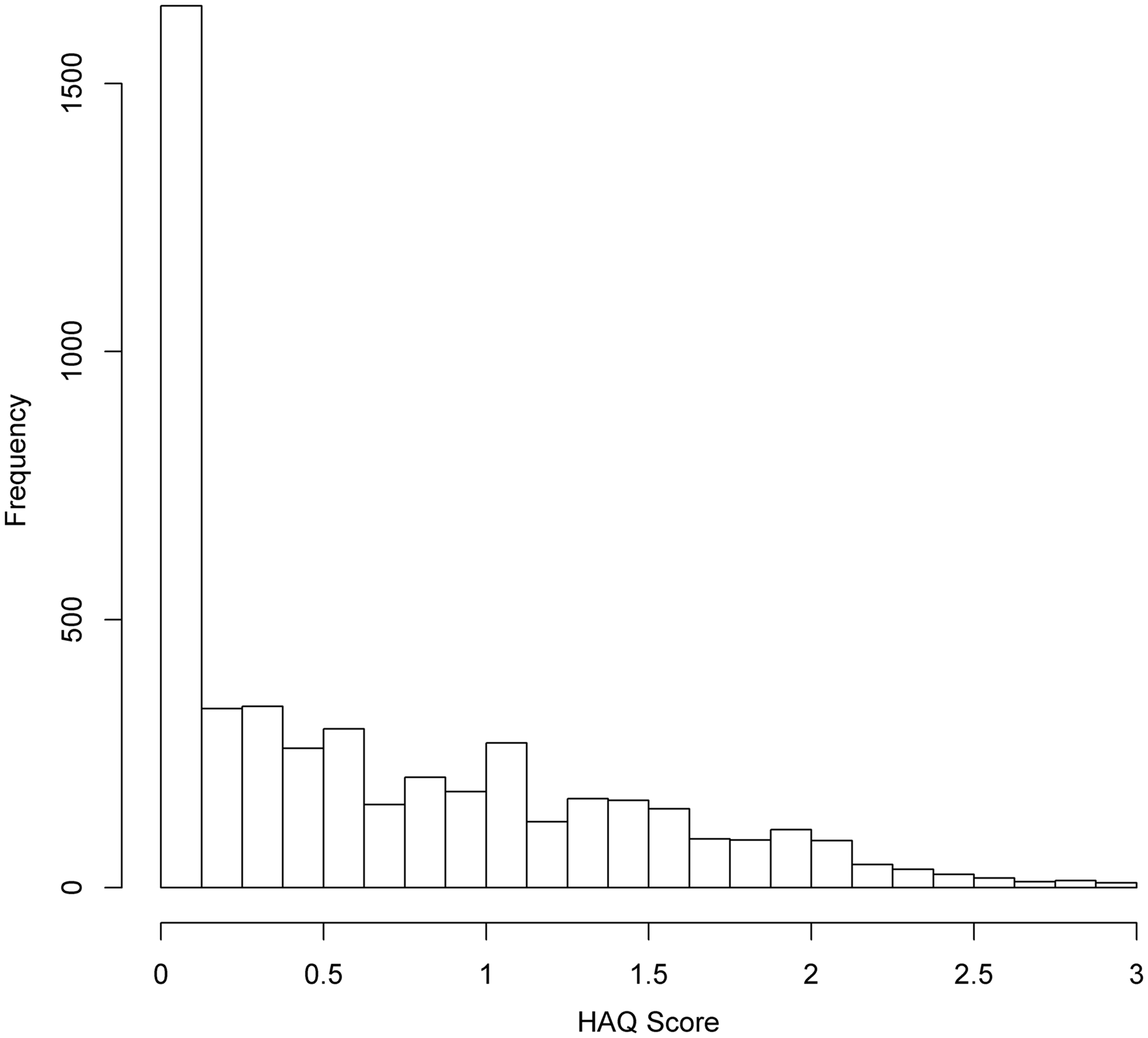
The HAQ scores of 698 patients observed longitudinally at the University of Toronto PsA clinic were considered for this analysis. Figure 1 shows the frequencies of HAQ scores from these patients. From Figure 1, it is evident that a large proportion of zeros exist in this data set (1526/4811 = 0.32). The clumping at zero, together with the continuous distributed outcomes for the non-zero values, suggests that the HAQ score can be viewed as a semicontinuous outcome. Su et al.12,13 considered two-part models with patient-specific random effects for analysing an earlier version of this PsA data set. In this paper, we relax the assumption of constant patient-specific random effects to patient-specific stochastic processes and consider the extent to which they improve understanding of the disability process. This includes making easy interpretable inference on the overall marginal mean HAQ scores, a concept that has not been considered before with stochastic processes models (see Section 6 for more details). On average, patients had 6.89 clinic visits (ranging from 2 to 20) with mean inter-visit and follow-up times of 1 year and 5 months (standard deviation (SD) of 1 year and 1 month) and 8 years and 3 months (SD of 5 years and 10 months), respectively.
Frequencies of HAQ scores in our data.
3 Model
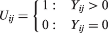
Let Yij () denote the semicontinuous response from patient i at time tij (), where tij represents the time of the jth observation from patient i. Because of true zeros, it is natural to decompose the response into
and , where is a monotonic function such that and is positive and approximately Gaussian with constant variance . For convenience, the model for Uij is referred to as the binary component, while the model for is referred to as the continuous component.
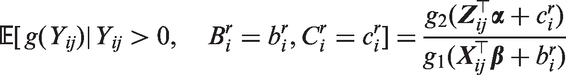
We now describe the flexible modelling framework. Let and be column vectors of covariates that influence the probability of Yij > 0 and the mean of , respectively. Then conditional on correlated patient-specific random effects and correlated stochastic processes , where the random effects are assumed independent of the stochastic processes, we model Uij as Bernoulli with response probability
where is the cumulative distribution function of a standard Gaussian distribution (i.e. probit model), and as Gaussian with mean and constant variance (i.e. linear mixed effect model on ). Here, and are column vectors of regression coefficients. The patient-specific random effects allow patients to have a consistently high or low probability of having disability and a consistently high or low mean for the non-zero HAQ scores across time. While the patient-specific stochastic processes can capture serial correlation and non-predictable changes in unobserved heterogeneity.9
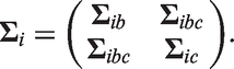
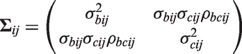
We assume follows a bivariate normal distribution with mean vector zero and
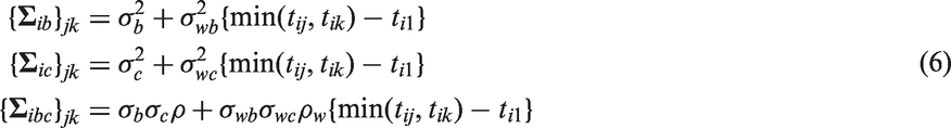
where and are variance parameters and ρ is the correlation between and . Furthermore, we consider two classes of stochastic processes for that are subsequently described. For convenience, define and , i.e. the patient-specific random effects and are absorbed into the stochastic processes and , respectively, and let the covariance matrix of be
3.1 Correlated Gaussian processes
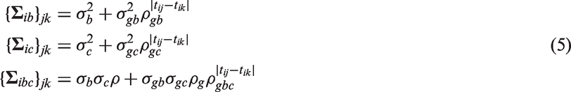
The first and most general model that we consider is defined when are correlated stationary Gaussian processes. That is the model proposed by Albert and Shen8
where and are variance parameters, ρg is the correlation between the Gaussian processes at the same time point, and ρgb, ρgc, ρgbc are the degradation parameters governing the serial correlation within and between processes, respectively. Following Albert and Shen,8 the processes and are taken to be exchangeable Ornstein-Uhlenbeck (EOU) processes, and the model containing these processes is called the general model, i.e. (1–3). Some special cases of the general model are
Shared EOU process model when ,
Correlated OU processes model when ,
Shared OU process model when and ,
Correlated random effects model when ,
Shared random effect model when and ,
where θ is a parameter to be estimated.
3.1.1 Remarks on ρgb, ρgc and ρgbc
Although the general model is very flexible, it will not always be mathematically valid. Let the covariance matrices and have (j, k)th entry and respectively, i.e. described by equation (3). If ρgb, ρgc and ρgbc are unconstrained (as specified by Albert and Shen8), the matrix where
will not in general be a valid covariance matrix since , although symmetric, is not constrained to be positive semi-definite and therefore and will not necessarily form a jointly Gaussian process. The primary difficulty results when ρg (the correlation between and at each time t) is close to one because the processes and are similar and therefore it will not be plausible for them to degrade at vastly different rates (i.e. for ρgb, ρgc and ρgbc to be vastly different). A reasonable approximation in this situation would be to constrain the degradation and cross degradation parameters to be same, specifically . This constraint would then enforce to be a valid covariance matrix since the Schur component , where has (j, k)th entry , is constrained to be positive semi-definite. The resulting correlation structure would then be
In the motivating application, ρg was estimated close to one. Slight deviations from the correlation structure described by equation (4) (for example and where ) resulted in non-positive semi-definite matrices for various , and therefore the model fitting procedure was problematic. Note that a further simplification would be to constrain (in addition to ), this would result in the shared EOU process model. If, however, ρg takes a smaller value, and therefore the two Gaussian processes are less correlated, it would then be more plausible for the Gaussian processes to degrade at different rates. Hence, having unconstrained degradations parameters will likely be less problematic.
For completeness, note that
3.2 Correlated random walks
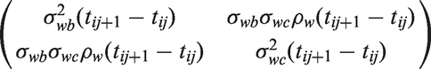
The second model structure that we consider is defined when are correlated continuous-time random walks. That is the model proposed by Ghosh and Albert.9 Specifically, define sequentially to be bivariate normal with mean and covariance matrix
In addition are initiated at realisations of the patient-specific random effects. Here, and ρw are variance and correlation parameters that quantify serial correlation (both within and across processes). This model will be denoted by a correlated random walks (CRW) model and it contains as special cases.
Shared random walk model when ,
Correlated random effects model when ,
Shared random effect model when and .
Although the CRW model is less flexible than the general model, it has the advantage, from its sequential construction, of always being well defined even when the parameters are unconstrained (apart from the usual constraint that correlation parameters have modulus less than or equal to unity). Moreover
4 Efficient maximum likelihood estimation procedure for stochastic processes models
This section describes our efficient maximum likelihood estimation procedure for the flexible models described in Section 3. Firstly, in Section 4.1, we describe a generic likelihood function for all of the described models. The multivariate normal identity that can be used to evaluate certain multi-dimensional integrals in terms of a multivariate normal cumulative distribution function is introduced in Section 4.2. Finally, in Section 4.3, we outline how to apply the multivariate normal identity in Section 4.2 to the generic likelihood function in Section 4.1, thus culminating in a computationally efficient likelihood. For completeness, we also provide computational simplifications for correlated stochastic processes models in the appendix.
4.1 Likelihoods
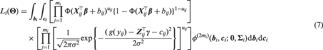
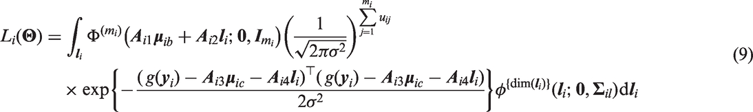
For ease of exposition, we describe the likelihood contribution from patient i. The likelihood can then be obtained by taking the product of all likelihood contributions from each patient. Firstly, we consider models that contain two (correlated) stochastic processes. For these models, the likelihood contribution from patient i is
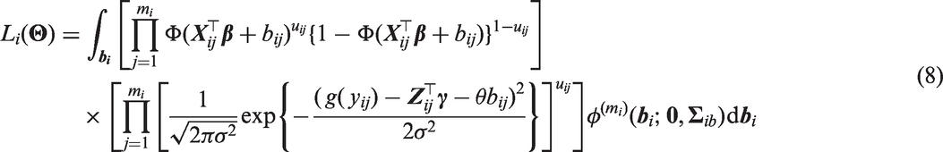
where is a vector comprising all of the unknown parameters, , is an m dimensional multivariate normal density with mean vector and covariance matrix , and is defined by either equation (5) or equation (6). Similarly, for models containing a single stochastic process (i.e. shared process models), the likelihood contribution from patient i is
where can again be obtained from equation (5) or equation (6). We now define our generic likelihood contribution from patient i which encompasses all of the described models. Throughout we apply the following notation: and are vectors with all entries being zero and one respectively, is a matrix with diagonal elements v and zero otherwise, and is a d × d identity matrix. We also follow the convention that binary operations with a scalar and vector or matrix argument and unary operations with a vector argument are performed element-wise. In matrix form, we have
where , and are matrices with . Here represents the distribution function of and is a (to be specified) column vector of random effects. Note that equation (9) has resulted from repeated application of the identity .
The likelihood contribution from patient i, , is then obtained by specifying the vector of random effects and its covariance matrix together with the matrices and which describe how the random effects act on the binary and continuous components of the model. For (7), and . While for equation (8), and . Similarly, for the correlated random effects model, and , and for the shared random effect model, li = bi, and .
4.2 Multivariate normal identity
In order to evaluate the likelihood described by equation (9), we derive a multivariate normal identity that makes use of a property of the multivariate normal distribution and the standard marginal cumulative distribution function identity. Firstly, suppose that follows a multivariate normal distribution with mean vector where and are vectors and and are vectors, respectively. Furthermore, suppose that the covariance matrix of is the matrix where the first k1 rows of is the matrix and the remaining k2 rows of is the matrix respectively. It is a well-known result that where the right-hand side is the product of the conditional density of and the marginal density of . By applying the standard marginal cumulative distribution function identity where the integrand is based on the right-hand side of the above result, we obtain the multivariate normal identity:
by noting that the marginal distribution of is multivariate normal with mean vector and covariance matrix .
Returning to the application, the general idea is to rearrange equation (9) to take the form of the right-hand side of equation (10), and then to use equation (10) to compute the integrations over the random effects in terms of an mi dimensional normal cumulative distribution function. Because there exists efficient implementations of the multivariate normal cumulative distribution function, this approach will allow for the efficient computation of the generic likelihood. We note that Barrett et al.15 used equation (10) to obtain computationally efficient likelihoods of flexible models that jointly consider longitudinal and time to event outcomes. Equation (10) also arises frequently in results concerning the multivariate skew normal distribution.16–19
4.3 Re-expressing the likelihoods
This section demonstrates how equation (9) (the likelihood contribution from patient i) can be re-expressed. We firstly consider the integrand terms resulting from the continuous component and random effects. That is
By completing the square in (see the appendix for more details), equation (11) can be rearranged as
where
and
is independent of . Substituting equation (12) into equation (9), we consider the integral (ignoring )
We can re-express the argument and covariance matrix of the multivariate normal distribution function in equation (15) as
Therefore equation (15), after applying the multivariate normal identity (described equation (10)), is equivalent to
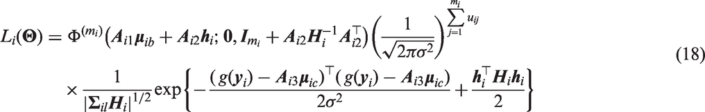
Based on the above expressions, the likelihood contribution from patient i can now be re-expressed as
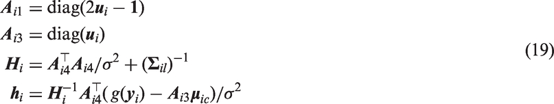
where
and or with and defined by the specified model.
From equations (18) and (19), it is now evident that evaluating the integrations involved in reduces to computing the cumulative distribution function of a multivariate normal distribution. This can be performed efficiently, for example by using the R20 package mnormt.21 The model fitting procedure is then completed by maximizing the log-likelihood, for example by using the BFGS22 optimization technique, to obtain parameter estimates and asymptotic standard errors (from the observed Fisher information matrix) of model parameters.
5 Application: Patient-specific inference
Using the estimation procedure described in Section 4, we demonstrate how patient-specific inference on the probability of being disabled and the transformed mean HAQ score conditional on disability can be obtained. Specifically, how a unit change in covariate values impacts these quantities for any specific patient. We consider the covariate effects of the number of clinically damaged joints (time-dependent), the number of actively inflamed joints (time-dependent), sex (coded as 1 for males and 0 for females), arthritis duration in years (time-dependent), and age at onset of arthritis in years (standardise). Following Su et al.,12,13 no transformation was applied to the non-zero HAQ scores, i.e. g(y) = y.
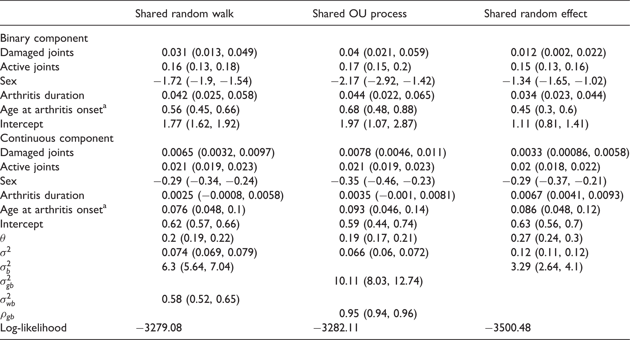
Initially, models with two stochastic processes were fitted to the HAQ data. This resulted in large estimated correlation parameters between the random effects (i.e. ) and stochastic processes for both the correlated Gaussian processes and random walks cases (i.e. ρg and ). These results therefore suggested a single stochastic process would be sufficient for describing the data. The shared EOU model was then fitted. However, the analysis provided evidence for model over-parameterisation as appeared to converge at virtually zero and a positive-definite observed Fisher information matrix could not be attained (even when a considerably smaller tolerance level than the default was specified for the computation of multivariate normal probabilities). We therefore considered the shared random walk and OU process models, and for comparative purposes, the shared random effect model. The models containing stochastic processes were fitted using the likelihood described by equations (18) and (19), while the shared random effect model was fitted using numerical integration (since only a single integration per patient is required). The same parameter estimates for the shared random effect model were obtained when equations (18) and (19) were used in the model fitting procedure.
Table 1 presents the results of the fitted models. Across the models, the covariate effects on the mean conditional on disability are seen to be relatively similar as the confidence intervals generally overlap. In addition, the models are in agreement with regard to the association of each covariate apart from arthritis duration. Arthritis duration is statistically significant in the shared random effect model but is not statistically significant in the models that incorporate stochastic processes. It is interesting to note that there are strong agreements regarding the covariate effect of the number of active joints (similar parameter estimates across models and relatively narrow confidence intervals). The models indicate an additional actively inflamed joint will increase the mean HAQ score conditional on disability by approximately 0.21 for any specific patient. For the binary component, the covariate effects are again seen to be relatively similar due to the overlapping confidence intervals. Their interpretation through the direction of association and statistical significance are also consistent across models. The covariate effects from the shared random effect model does, however, consistently demonstrate attenuation to the null when compared to the other models with stochastic processes.
Table displaying patient-specific effects and corresponding 95% Wald intervals on the probability of being disabled and the mean HAQ score conditional on disability.
Denotes the standardised version of the covariate.
A generalized likelihood ratio test of and produced p values of < 0.001 therefore suggesting preference towards the shared random walk and OU process models respectively when compared to the shared random effect model. Since the shared random walk and OU process models contain the same number of parameters, information criteria, such as AIC, would indicate (weakly) that the shared random walk model is preferable. It is also worth noting that the heterogeneity parameter in the binary component (i.e. or ) is significantly lower in the shared random effect model. For this model, this parameter governs both the heterogeneity and correlation due to repeated measurements and therefore in light of greater unaccounted heterogeneity (compared to the models with stochastic processes), less correlation is expected.23 In the continuous component, where also accounts for heterogeneity, a smaller difference between the heterogeneity parameters (i.e. or ) is seen; in the order of the models displayed in the table (from right to left), the heterogeneity parameters are 0.24, 0.36 and 0.25, respectively.
6 Modelling the overall marginal mean
In many cases, it is of interest to obtain population-based inference in addition/as opposed to patient-specific inference. For example, for strategic public health policy purposes, it would be more clinically meaningful to obtain covariate effects on quantities of interest after averaging over all patients. Currently, the proposed models are parametrised to allow easily interpretable patient-specific covariate effects, those with and , to act on the patient-specific mean of the transformed positive values (i.e. ) and the patient-specific probability of a having a positive value (i.e. ). However, under this parametrisation, it no longer becomes straightforward to obtain easily interpretable population-level covariate effects on the marginal mean of the transformed positive values (the mean of the transformed positive values after averaging over all bij and cij, i.e. ) since it is a highly non-linear function of the linear predictors in the binary and continuous components.5 Thus, the effect of a single covariate is generally interpreted by fixing other covariates at certain values.8 This problem remains even when population-level covariate effects on the overall marginal mean of the transformed values (i.e. ) are of primary interest, which has strongly been argued as an important target of inference;24 it is estimated using data from the same patients over time (unlike ) and it is a measure of the undecomposed outcome. We reiterate that in considering the overall marginal mean of the transformed values as a target of inference, we assume that the monotonic transformation function is such that and is positive and approximately Gaussian with constant variance .
In order to obtain population-based inference on the overall marginal mean of the transformed values, Smith et al.4 proposed the following model parameterisation
where and are monotonic link functions and are, as before, zero mean bivariate normal patient-specific random effects. Recall that transformation and link functions differ in that transformation functions are applied prior to modelling. In their specific context, Smith et al.4 considered the identity transformation for but allowed the positive values of Yij to follow a log-skew-normal distribution. Under this parametrisation, for a suitably chosen link function such as being the identity or log link, it is implicit that easily interpretable covariate effects on the overall marginal mean of , can now be obtained. Smith et al.4 implemented this model by using a Bayesian estimation approach with
specified in the likelihoods defined by equation (7) or equation (8). Note that is no longer parametrised to be equivalent to a monotonic function of a linear predictor, as was specified before. While this approach for modelling the overall marginal mean is intuitive, it is clear that the multivariate normal identity in Section 4.2 can no longer be used to compute the integrations over the multi-dimensional random effects in the marginal likelihood. Thus, as mentioned in the introduction, implementation of such models can be computationally challenging, especially for our situation where it would be of interest to consider bij and cij (i.e. realisations of stochastic processes) instead of and (i.e. realisations of patient-specific random effects) in equation (20).
We now propose another method which would allow easily interpretable covariate effects to act on the overall marginal mean of . In contrast, this method facilitates the inclusion of stochastic processes because it retains the proposed efficient implementation procedure described in Section 4. To the best of our knowledge, there are no other methods in the literature that facilitates the practical implementation of stochastic processes models for directly modelling the overall marginal mean.
We first begin by computing the overall marginal mean of when
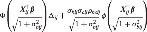
where Δij is a function of covariates (at the jth visit from patient i) and regression coefficients only. That is cij is now assumed to act additively on the mean of the transformed positive values and not on the overall mean of the transformed values as is the case in equation (20). For models with two processes, the overall marginal mean of is defined by
where
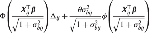
and and ρbcij are the variances and correlation of and , respectively. Similarly, the overall marginal mean for a shared process model is given by
Conveniently, these integrals can be computed analytically and this results in
and
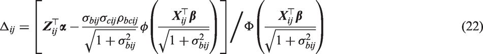
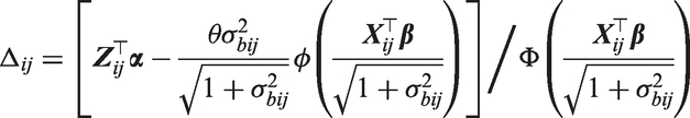
respectively. The derivation of the first overall marginal mean of (resulting from models with two processes) can be found in the supplementary material of Tom et al.,5 and the second overall marginal mean of is derived in the appendix. If we specify , we can then reparametrise
and
in the respective models. Thus, as in equation (20), offers easily interpretable covariate effects of on the overall marginal mean of (by definition). In particular, a unit change in components of will increase the overall marginal mean of by the respective components in . However, from equations (21) and (22), it is also evident that replacing with Δij in Section 4 will still allow the proposed efficient estimation procedure to be applied. It is also possible to reparametrise patient-specific covariate effects in the binary component in terms of population-level covariate effects , specifically , since it can be shown that . This relationship is easily proved. In the motivating application, this reparametrisation led to a numerically unstable optimization routine, therefore was estimated with obtained as and standard errors were calculated using the delta method.
6.1 Population-based inference
Using the parameterisations described in the previous subsection, we demonstrate how population-based inference on the probability of being disabled and the overall marginal mean HAQ score can be obtained. Specifically, on averaging across patients, how a unit change in covariate values impacts these quantities. For illustrative purposes, the same covariates as those considered in the patient-specific case are considered. Note that for generalized linear models, conditional and marginal covariate effects will generally differ unless certain random effects distributions and link functions are chosen.25
As mentioned, marginal covariate effects on the probability of being disabled, , were obtained from with and (the variance of ) estimated using the model fitting procedure. The shared OU process and random effect models, where does not depend on j (or i) for these models, were considered. For models with random walks, varies with j and therefore will have a time-dependent interpretation. For simplicity, these models are not considered. The shared random effect model was fitted using the parameterisation described by equation (20), with and , and using the parameterisation described by equations (21) and (22), thus the same link functions are used and the inferences (at the population-level) from these models are comparable. These models will be denoted as shared random effect model-overall and -conditional respectively. Note that unlike at the population-level, the patient-specific assumptions from the shared random effect model-overall and -conditional are vastly different. The shared random effect-overall model assumes that the overall patient-specific mean, i.e. , has a linear form, namely . While the shared random effect-conditional model assumes that this quantity takes a particular non-linear form, namely . As before, the shared random effect models (both -overall and -conditional) were fitted using numerical integration and maximum likelihood estimation under the assumption that the positive values follow a normal distribution with constant variance.
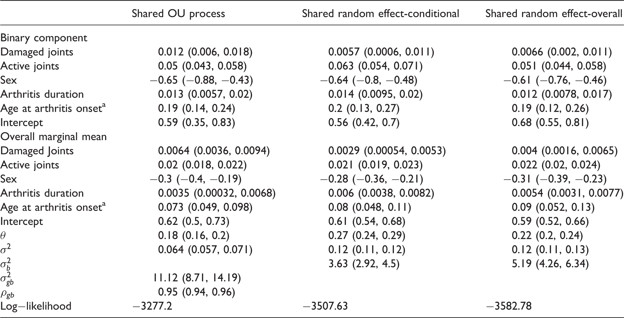
Table 2 presents the results. Population-level covariate effects on the overall marginal mean are seen to be relatively similar across models due to the considerable overlap in confidence intervals. All three models are in strong agreement regarding the population-level covariate effect of the number of active joints. That is, on average, patients with an additional actively inflamed joint have an overall mean HAQ score increased by approximately 0.02. In contrast to the patient-specific case, the population-level covariate effects on the probability of being disabled are now more consistent across models. A generalized likelihood ratio test of produced a p value of < 0.001 and therefore the shared OU process model is to be preferred over the shared random effect-conditional model. Log-likelihood values also indicate slight preference to the shared random effect-conditional model (−3507.63) over the shared random effect-overall model (−3582.78).
Table displaying population-level effects and corresponding 95% Wald intervals on the probability of being disabled and the overall marginal mean HAQ score.
Denotes the standardised version of the covariate.
7 Discussion
This paper reconsiders the flexible two-part models of Albert and Shen8 and Ghosh and Albert9 and proposes an efficient method of implementation. Specifically, the problem of integrating over high dimensional random effects is replaced by evaluating the cumulative distribution function of a multivariate normal distribution. This leads to efficient algorithms being employed and results in only an optimization procedure being required for model fitting. Furthermore, while retaining the flexibility of including stochastic processes and the practicality of an efficient model fitting procedure, this paper also provides model parameterisations which allow easily interpretable covariate effects to act on the overall marginal mean. The proposed methodology was applied to a psoriatic arthritis data set with extensive follow-up information.
Through their application and a simulation study, Albert and Shen8 demonstrated that overall conditional means (conditional on realisations of stochastic processes) may suffer from bias if serial correlation is present but a shared random effect model is used instead. Furthermore, as the shared random effect model becomes more misspecified (ρgb decreases from one), the degree of bias increases. However, under the same set-up, overall marginal means were less susceptible to bias. In the motivating application, the estimated degradation parameters from the shared OU process models were in both applications (Sections 5 and 6.1). The reasonably high estimated correlation may therefore explain why the shared random effect model was a reasonable approximation in terms of estimating regression coefficients, although it was substantially the worst fitting model.
Preliminary analyses suggested shared process models were reasonable for our data since and when the described bivariate processes models were fitted. Although this may not be surprising as both parts of the model are describing the same response process, it is worth noting that the estimated correlation parameter (between processes) can in principle take a value between as evidenced in other works.7,9 Our preliminary analyses also demonstrated the need for careful evaluation of models fitted as problems with over fitting may arise. This was evident when the estimated random variation parameter was estimated to be virtually zero (i.e. ) and the observed Fisher information matrix was non positive-definite, even when a considerably smaller tolerance level than the default was specified for computing multivariate normal probabilities.
As mentioned in Section 6, the proposed model parameterisations were motivated by making inference on the overall marginal mean. In this regard, covariate effects (both patient-specific and population-level) on the mean of the positive values and its correlation structure were assumed not of interest. If the mean of the positive values is of primary interest, it would be more sensible to directly use equations (18) and (19), as in Section 5, to obtain patient-specific effects or derive a similar parameterisation, as in Section 6, to obtain population-level effects.
A limitation of the current framework is that it is based on the assumption is approximately Gaussian with constant variance . Specifically, in situations where is required to be complex so that this assumption will at least approximately hold, the resulting inferential targets will no longer be intuitively interpretable owing to the complexity of the transformation function. One approach that may weaken the need to assume normality of , particularly when the outcome exhibits a large amount of right skewness (e.g. medical expenditures), would be to make the alternative assumption follows a log-normal distribution. This may allow less complex and hence more interpretable transformation functions to be applied to the outcome without having to strongly violate the assumption on . Under this alternative assumption, we provide details in the supplementary materials of how easily interpretable inference on the overall marginal mean and on the mean of the positive transformed outcomes can be obtained with computationally efficient likelihoods. Similar techniques to those in the supplementary materials can also be used when the assumption follows a log-skew-normal distribution is of interest. Although this comes at the cost of having an increased number of integrations in the marginal likelihood.
Finally, the model described by equations (18) and (19) with possible simplifications described in Appendix 2 is very general. Although it was derived in the context of longitudinal semicontinuous data, it contains the model described by Barrett et al.15 for the longitudinal and survival outcomes setting and implicitly provides a model for clustered cross-sectional semicontinuous data, where the index (i, j) specifies the jth outcome from the ith cluster. The multivariate normal identity described in Section 4.2 can also facilitate the fitting of flexible models describing clustered binary data and continuous bounded outcome data.14 However, it should be noted that care is required when specifying an appropriate/suitable correlation structure. Particularly, the covariance matrix must be constrained to be symmetric and positive semi-definite otherwise the model fitting procedure will likely be problematic, as was found here. For these alternative situations, the proposed methodology does nevertheless offer a strong basis, especially with regard to implementation, for the developing of flexible models.
Supplemental Material
Supplemental material for Two-part models with stochastic processes for modelling longitudinal semicontinuous data: Computationally efficient inference and modelling the overall marginal mean
Supplemental Material for Two-part models with stochastic processes for modelling longitudinal semicontinuous data: Computationally efficient inference and modelling the overall marginal mean by Sean Yiu and Brian DM Tom in Statistical Methods in Medical Research
Footnotes
Acknowledgments
We are grateful to Professor Vernon T. Farewell for providing general discussions on this research. We also acknowledge the patients in the Toronto Psoriatic Arthritis Clinic.
Declaration of conflicting interests
The author(s) declared no potential conflicts of interest with respect to the research, authorship, and/or publication of this article.
Funding
The author(s) disclosed receipt of the following financial support for the research, authorship, and/or publication of this article: This work was financially supported by the UK Medical Research Council [Unit program numbers U105261167 and MC_UP_1302/3].
Appendix 1. Rearranging equation ( 11 )
Appendix 2. Simplification for correlated stochastic processes model
Appendix 3. Overall marginal mean of shared process model
References
1.
OlsenMKSchaeferJL. A two-part random effects model for semicontinuous longitudinal data. J Am Stat Assoc2001; 96: 730–745.
2.
XieHMcHugoGSenguptaAet al.A method for analyzing longitudinal outcomes with many zeros. Ment Health Serv Res2004; 6: 239–246.
3.
SmithVAPreisserJSNeelonBet al.A marginalized two-part model for semicontinuous data. Stat Med2014; 33: 4891–4930.
4.
SmithVANeelonBPreisserJSet al.A marginalized two-part model for longitudinal semicontinuous data. Stat Meth Med Res2015; July: 1–24.
5.
TomBDMSuLFarewellVT. A corrected formulation for marginal inference derived from two-part mixed models for longitudinal semi-continuous data. Stat Methods Med Res2016; 25: 2014–2020.
6.
HallDBZhangZ. Marginal models for zero-inflated clustered data. Stat Model2004; 4: 161–180.
7.
ToozeJAGrunwaldGKJonesRH. Analysis of repeated measures data with clumping at zero. Stat Meth Med Res2002; 11: 341–355.
8.
AlbertPSShenJ. Modelling longitudinal semicontinuous emesis volume data with serial correlation in an acupuncture clinical trial. J R Stat Soc: Ser C2005; 54: 707–720.
9.
GhoshPAlbertPS. A Bayesian analysis for longitudinal semicontinuous data with an application to an acupuncture clinical trial. Comput Stat Data Anal2009; 53: 699–706.
10.
BruceBFriesJF. The Stanford health assessment questionnaire: dimensions and practical applications. Health Qual Life Outcomes2003; 1: 1–20.
11.
HustedJATomBDFarewellVTet al.A longitudinal study of the effect of disease activity and clinical damage on physical function over the course of psoriatic arthritis: does the effect change over time?Arthritis Rheum2007; 56: 840–849.
12.
SuLTomBDFarewellVT. Bias in two-part mixed models for longitudinal data. Biostatistics2009; 10: 374–389.
13.
SuLTomBDFarewellVT. A likelihood-based two-part marginal model for longitudinal semicontinuous data. Stat Meth Med Res2015; 24: 194–205.
14.
HutmacherMMFrenchJLKrishnaswamiSet al.Estimating transformations for repeated measures modelling of continuous bounded outcome data. Stat Med2010; 30: 935–949.
15.
BarrettJDigglePHendersonRTaylor-RobinsonD. Joint modelling of repeated measurements and time-to-event outcomes: flexible model specification and exact likelihood inference. J R Stat Soc: Ser B2015; 77: 131–148.
16.
AzzaliniA. A class of distributions which includes the normal ones. Scand J Stat1985; 12: 171–178.
17.
AzzaliniA. The skew-normal distribution and related multivariate families (with discussion). Scand J Stat1985; 32: 159–200.
ArnoldBC. Flexible univariate and multivariate models based on hidden truncation. J Stat Plan2009; 139: 3741–3749.
20.
R Development Core Team. R: a language and environment for statistical computing. R Foundation for Statistical Computing: Vienna, Austria, http://www.R-project.org, ISBN 3-900051-07-0 (accessed 6 May 2017)..
BroydenCG. The convergence of a class of double-rank minimisation algorithms. J Inst Math Appl1970; 6: 76–90.
23.
HendersonRShimakuraS. A serially correlated gamma frailty model for longitudinal count data. Biometrika2003; 90: 355–366.
24.
AlbertPS. Letter to the editor. Biometrics2005; 47: 879–881.
25.
DigglePHeagertyPLiangKYet al.Analysis of longitudinal data, New York: Oxford University Press, 2002.
26.
OwenDB. A table of normal integrals. Commun Stat B Simul1980; 9: 389–419.
Supplementary Material
Please find the following supplemental material available below.
For Open Access articles published under a Creative Commons License, all supplemental material carries the same license as the article it is associated with.
For non-Open Access articles published, all supplemental material carries a non-exclusive license, and permission requests for re-use of supplemental material or any part of supplemental material shall be sent directly to the copyright owner as specified in the copyright notice associated with the article.