Sage Journals: Discover world-class research

Abstract

The use of multiple imputation has increased markedly in recent years, and journal reviewers may expect to see multiple imputation used to handle missing data. However in randomized trials, where treatment group is always observed and independent of baseline covariates, other approaches may be preferable. Using data simulation we evaluated multiple imputation, performed both overall and separately by randomized group, across a range of commonly encountered scenarios. We considered both missing outcome and missing baseline data, with missing outcome data induced under missing at random mechanisms. Provided the analysis model was correctly specified, multiple imputation produced unbiased treatment effect estimates, but alternative unbiased approaches were often more efficient. When the analysis model overlooked an interaction effect involving randomized group, multiple imputation produced biased estimates of the average treatment effect when applied to missing outcome data, unless imputation was performed separately by randomized group. Based on these results, we conclude that multiple imputation should not be seen as the only acceptable way to handle missing data in randomized trials. In settings where multiple imputation is adopted, we recommend that imputation is carried out separately by randomized group.

Keywords

Missing data multiple imputation clinical trials linear mixed model intention to treat

1 Introduction

Research articles and guidance documents have emphasized the role of prevention in minimizing the impact of missing data,^1–4 but most randomized controlled trials (RCTs) have some missing data.⁵ Given the potential for biased and inefficient treatment effect estimates, it is crucial that missing data are handled appropriately during the analysis.

All statistical analyses involve assumptions about the mechanism responsible for the missing data. Rubin⁶ introduced three classes of mechanisms for missing data: missing completely at random (MCAR), where the probability of missingness is unrelated to observed or unobserved data; missing at random (MAR), where the probability of missingness is unrelated to unobserved data conditional on observed data; and missing not at random (MNAR), where the probability of missingness depends on unobserved data conditional on observed data. Since MAR and MNAR cannot be distinguished from observed data, it is essential that the assumptions of the analytic approach are scientifically plausible and clearly stated.^7,8 To assess the robustness of findings to the assumption made about the missing data mechanism in the primary analysis of an RCT, additional sensitivity analyses are strongly recommended.^7–11

Multiple imputation (MI)⁶ is a statistical approach to handling missing data that has been widely adopted due to its flexibility and ease of implementation.^12,13 MI involves fitting a statistical model to the observed data and using it to estimate values for the missing data. To incorporate missing data uncertainty, multiple values are imputed for each missing observation, producing multiple complete datasets. Following analysis of these datasets using standard complete data techniques, the multiple parameter estimates are combined using Rubin's rules⁶ to give a single MI estimate. Standard implementations of MI assume that data are MAR, although it can also be applied under an MNAR assumption.⁶ Provided the assumption about the missing data mechanism is met and models used for imputation and analysis are correctly specified, MI produces consistent and asymptotically efficient parameter estimates with nominal coverage.⁶ Of the various methods of imputation available, MI based on the multivariate normal distribution¹⁴ and MI by chained equations^15–17 are most commonly used in RCTs.¹⁸

With the use of MI in RCTs rising dramatically in recent years,^12,18,19 editors and journal reviewers may expect to see MI used to handle missing data. Indeed, we are aware of several recent instances where reviewers have pushed with little justification for trial data to be re-analysed using MI. However, whether MI should be viewed as the gold standard approach for handling missing data in RCTs is questionable. Importantly, results derived in general regression settings supporting the use of MI may not be applicable to RCTs. Unlike observational studies, the key exposure in RCTs (randomized group) is always observed and known to be independent of baseline covariates. In addition, missing data occur primarily in the outcome variable, although baseline covariates may also have missing data. Under these conditions, some of the value of MI may be lost and other methods of analysis may be preferable.

Another uncertainty around the use of MI in RCTs is whether imputation is best carried out across all participants or separately by randomized group. If subgroup analyses are of interest, it is essential that interaction terms are accounted for in the imputation process to avoid biasing interaction tests towards the null. Rather than specifying interaction terms within the imputation model, several authors have recommended fitting separate imputation models within each randomized group.^11,20–22 This strategy is appealing due to its simplicity and ability to facilitate subgroup comparisons for any baseline covariate included in the imputation model. Unfortunately its performance is not well understood, and it is unclear how imputation should proceed when subgroup analyses are not of interest and the intention is to only produce average treatment effects (ATEs) from main effects models.

This article describes the performance of MI in the RCT setting, covering the common scenarios of missing data in an outcome measured once or repeatedly over time and missing data in a baseline covariate. Using a series of illustrative data simulations and a case study, we compare MI with other standard approaches for handling missing data and explore the merits of imputing overall and separately by randomized group. Throughout we assume that missing data are unplanned rather than by design, and that interest lies in estimating the effect of treatment according to the intention to treat (ITT) principle. If treatment discontinuations occur, we therefore assume the aim is to estimate a ‘de facto' estimand^23,24 and that data are equally available before and after treatment discontinuations; we consider the case where data cannot be collected after treatment discontinuation in the discussion. For missing outcome data, we restrict attention to settings where they are assumed to be MAR, since this assumption is often made in the primary analysis of an RCT and corresponds with the standard implementation of MI.

The remainder of the article is structured as follows. Section 2 describes issues in adhering to the ITT principle in the presence of missing data and implications for the use of MI in RCTs. Section 3 defines key notation and outlines general simulation methods for evaluating the performance of MI. Section 4 focuses on the performance of MI for handling missing data in an outcome measured at a single time point. Section 5 considers missing data in an outcome measured repeatedly over time and the use of auxiliary variables in MI, while Section 6 focuses on missing data in a baseline covariate for adjustment. Section 7 shows the application of MI to the DINO trial. Finally, conclusions and general recommendations are provided in Section 8.

2 Intention to treat and missing data

The goal of ITT, or analyzing as randomized, is to maintain the balance in prognostic factors achieved by randomization, which is critical for avoiding selection bias and establishing causation.^25,26 In addition to preserving the benefits of randomization, an ITT analysis may better inform changes in subsequent clinical practice, where patients do not always comply with treatment. Following the ITT principle entails estimating the ITT estimand, which is defined as the average effect of randomization, irrespective of treatment received, over all randomized individuals.²⁷ Due to fluctuating use of the term ITT, this has more recently been described as a de facto estimand.^23,24 Interest in the ITT estimand has implications both for trial conduct and analysis. First, attempts should be made to collect outcome data on all randomized participants, irrespective of adherence to the protocol.^7,8,27 For example, outcome data should still be retrieved for participants that discontinue or switch treatments during the course of a trial. Second, all collected outcome data should be included in the analysis, including data from participants that deviate from the protocol.^7,8,27 Although there are settings where it may not be feasible to measure outcomes following a protocol deviation, or where exclusion of collected outcome data may be justifiable, we do not tackle these scenarios in this article.

Despite efforts to collect data on all randomized participants, invariably there will be some missing data. Exactly what constitutes an ITT analysis in the presence of missing data has been much debated.²⁸ Some researchers have suggested that missing outcome data ought to be imputed, so that the full randomized sample can be included in the analysis.^26,29,30 Others have argued that imputation is unnecessary and that an ITT analysis need only provide a valid estimate of the ITT estimand.^7,8,31 Given recent commentary on the importance of defining and validly estimating the causal estimand of interest,⁸ and noting that none of the current guidance documents strictly recommend imputing missing outcomes, we adopt the second view. In differentiating between competing statistical methods, we therefore focus on their capacity to provide an unbiased and precise estimate of the ITT estimand rather than their ability to include all randomized participants.

3 Methods

3.1 Setting

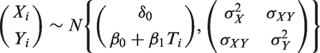
Let Y_i and X_i define values for the ith participant (i = 1 to n) on an outcome variable and a baseline variable, respectively. Assume the ith participant is randomized independently to treatment group T_i (0 = control, 1 = new treatment) with probability 0.5. Let $M_{Yi}$ and $M_{Xi}$ denote whether Y_i and X_i are missing or observed (1 = missing, 0 = observed). In the absence of missing data, suppose the adjusted analysis model

g (μ_{i}) = β_{0} + β_{1} T_{i} + β_{2} X_{i}

(1)

is of interest, where

μ_{i} = E (Y_{i} | T_{i}, X_{i})

and g is an appropriate link function. Of principal importance is the (adjusted) treatment coefficient

β_{1}

. Note we focus primarily on adjusted estimates in this article, since adjustment for pre-specified baseline covariates is common and can lead to substantial increases in power for testing the effect of treatment.^32,33 As conclusions about treatment are typically based on main effects models,¹ we also restrict attention to analysis models that do not include interaction terms.

3.2 MI

In the first stage of MI, multiple values (m > 1) for each missing observation are independently simulated from an imputation model. For missing data restricted to the outcome, the imputation model would typically regress observed values of Y on X and T. Additional auxiliary variables that are not in the analysis model can also be added to the imputation model to improve the prediction of missing values. Let $\hat{γ}$ denote the parameter estimates from the imputation model and $γ_{j}^{*}$ (j = 1 to m) random draws from the posterior distribution of $γ$ . For each random draw, missing values in Y are replaced by simulated values from the posterior predictive distribution of Y according to $γ_{j}^{*}$ . For missing data restricted to a baseline covariate, the imputation model instead describes the conditional distribution of X according to Y and T. If MI is performed separately by randomized group, T is omitted from the separate imputation models.

In the second stage of MI, the intended analysis is performed on each of the m complete datasets, in this case model (1). Let ${\hat{θ}}_{j}$ denote the estimate of $β_{1}$ from the jth imputed dataset and W_j the corresponding variance estimate. Using Rubin's rules,⁶ the combined MI treatment effect estimate $\hat{θ}$ is calculated as the mean of the m estimates, i.e. $\hat{θ} = 1 / m \sum_{j = 1}^{m} {\hat{θ}}_{j} .$ The variance is given by $var (\hat{θ}) = W + B (1 + 1 / m)$ , where $W = 1 / m \sum_{j = 1}^{m} W_{j}$ is the average within-imputation variance and $B = (m - 1)^{- 1} \sum_{j = 1}^{m} ({\hat{θ}}_{j} - \hat{θ})^{2}$ the between imputation variance. Hypothesis tests and confidence intervals can be obtained using a t-distribution with $v = (m - 1) [1 + W / (1 + m^{- 1}) B]^{2}$ degrees of freedom.

3.3 General simulation methods

Simulation studies were undertaken to describe the performance of MI for handling missing data in a univariate outcome (Section 4), a multivariate outcome (Section 5) and a baseline covariate (Section 6). For each scenario, 2000 datasets of size n = 600 were generated, with 300 observations allocated to each group. The sample size was chosen to be similar to that of a case study (see Section 7) and to represent a medium-sized trial. Three statistical methods were considered across all settings based on the adjusted analysis model (1): complete case analysis (CCA), MI performed overall and MI performed by randomized group. For MI, linear and logistic regression were used for the imputation of continuous and binary variables, respectively, with m = 50 imputations based on the rule of thumb that the number of imputations should at least equal the percentage of missing data.¹⁷ Completed datasets were analysed using linear and logistic regression as appropriate, with treatment effect estimates combined using Rubin's rules.⁶ Performance was evaluated in terms of bias, empirical standard error (SE), power and the coverage of estimated 95% confidence intervals. Based on 2000 simulated datasets, on 95% of occasions the coverage is expected to lie between 0.94 and 0.96 for a true coverage of 0.95. All analyses were performed in SAS version 9.3 (SAS Institute, Inc., Cary, North Carolina).

4 Missing data in a univariate outcome

When a univariate (once-measured) outcome is MAR conditional on fully observed covariates, a correctly specified CCA with covariate adjustment produces unbiased and efficient estimates of regression parameters.^34–36 It has also been shown that MI with a large number of imputations approximates a CCA in this setting, provided that imputation and analysis models are the same.³⁷ Using data simulation, we verify these results for RCTs, explore the implications of imputing overall or by randomized group and investigate settings where the analysis model is misspecified.

4.1 Correctly specified analysis model

Data were simulated from the model $Y_{i} = 0.30 T_{i} + β_{2} X_{i} + e_{i}$ , with X and e $\sim N (0, 1)$ . To assess whether model performance depended on the strength of association between X and Y, $β_{2}$ was varied so that $corr (X, Y | T) = 0.30 or 0.70$ . Since comparisons were insensitive to the treatment effect, $β_{1}$ was fixed at 0.30 to reflect a small effect size. Following generation of complete datasets, values in Y were set to missing according to three MAR mechanisms:

MAR X: Odds of missing Y increase by a factor λ per standard deviation (SD) increase in X.

MAR X + T: Odds of missing Y are λ times higher in the control group and increase by a factor λ per SD increase in X.

MAR X × T: Odds of missing Y are λ times higher for treatment group participants with $X \leq 0$ and for control group participants with $X > 0$ .

Each missingness mechanism was simulated using a logistic regression model, with λ = 1.5 or 2.5 to indicate weak and strong mechanisms, respectively, and with the model intercept varied to produce 20% (realistic) or 50% (extreme) missing data. This resulted in 24 simulation scenarios (12 missing data scenarios and two values for $β_{2}$ ). Supposing that X is a measure of disease severity, the MAR X and MAR X + T mechanisms might reflect settings where participants with more severe disease or randomized to the control group are more likely to have missing outcome data. The MAR X × T mechanism could apply in settings where treatment group participants with less severe disease are also more likely to have missing outcome data due to a perceived lack of need to continue treatment.

As expected, CCA, MI overall and MI by group all produced unbiased treatment effect estimates across the 24 simulation scenarios, with coverage probabilities remaining close to 0.95 throughout (range 0.94, 0.96). Compared to CCA, empirical SEs were on average 0.4% and 2.7% larger with MI overall and MI by group, respectively, which translated to an average loss of power of 0.8% for MI overall and 2.6% for MI by group. Figure 1 shows the performance of the various approaches in scenarios with 50% missing data, a strong MAR mechanism and where $corr (X, Y | T) = 0.70$ ; these more extreme scenarios were chosen to highlight differences between approaches. Results from an unadjusted CCA are also displayed for comparison. In all figures, note that error bars indicate estimation efficiency ( $\pm 1$ empirical SE). Unsurprisingly, MI offered no advantages over a CCA across the range of missingness mechanisms. Of note, unadjusted CCA produced biased estimates when the probability of missing data depended on X and T, with coverage dropping to 0.39 under the MAR X × T mechanism.

Figure 1.

Mean treatment effect estimates for 50% missing data in a continuous outcome, corr(X,Y|T) = 0.70, strong missing at random (MAR) mechanisms, correctly specified analysis model. Error bars correspond to empirical standard errors (±1 standard error) across 2000 simulated datasets.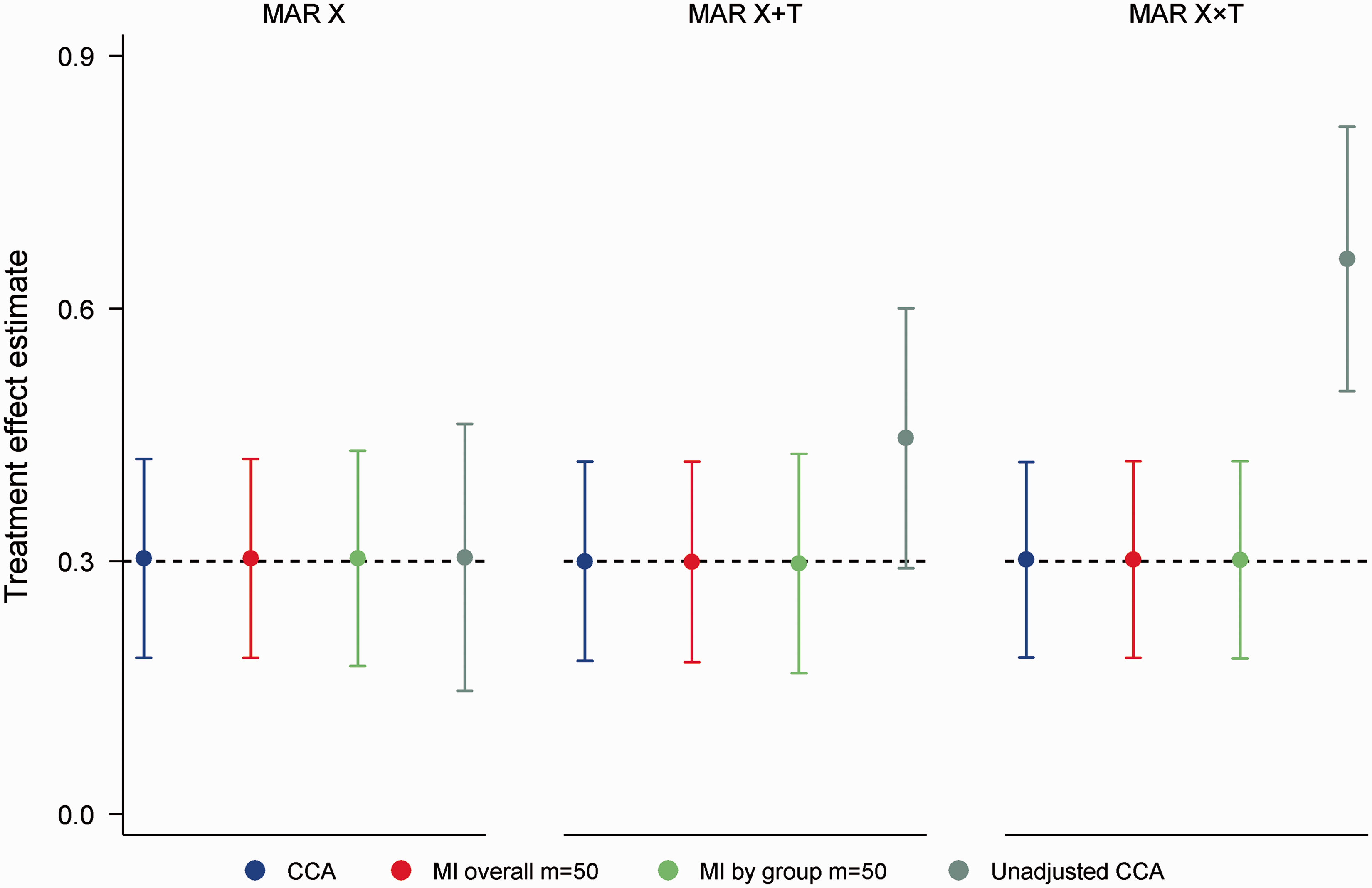

Similar results were obtained from a simulation study involving a binary outcome (online Appendix A).

4.2 Misspecified analysis model, continuous outcome

We now consider settings where an interaction between X and T is overlooked in favour of producing an estimate of the ATE. This approach is common in practice, since ATEs are commonly used to draw conclusions about treatment and are of greater relevance to policy-related questions.^1,38 Further, tests of interaction are often viewed as exploratory and can be underpowered.¹ For effect modification by discrete X, we assume that interest lies in estimating the ATE given by $\sum_{X} π_{X} α_{X}$ , where $π_{X} = P (X = x)$ and $α_{x}$ denotes the ITT estimand for $X = x$ .

Considering binary X with $π_{0} = π_{1} = 0.5,$ data were generated from the model $Y_{i} = β_{1} T_{i} + 0.30 X_{i} + β_{3} X_{i} T_{i} + e_{i}$ , where $e \sim N (0, 1)$ . Fixing the ATE at 0.30, we investigated both weak ( $β_{1} = β_{3} = 0.20$ or equivalently $α_{0} = 0.20, α_{1} = 0.40$ ) and strong ( $β_{1} = 0, β_{3} = 0.60$ or $α_{0} = 0, α_{1} = 0.60$ ) interaction effects between X and T. Following generation of complete datasets, values in Y were set to missing according to the mechanisms described in Section 4.1. Analysis model (1), misspecified due to the absence of the interaction term between X and T, was the substantive model of interest.

Across all simulation scenarios MI by group produced unbiased estimates of the ATE with nominal coverage (coverage range 0.94, 0.96). In contrast, CCA and MI overall produced biased estimates under the MAR X and MAR X + T mechanisms. Figure 2 illustrates performance for the MAR X mechanism in scenarios with 50% missing data. As seen in the figure, the bias of CCA and MI overall increased with the strength of the missing data mechanism and the degree of effect modification. For a strong missing data mechanism and a strong interaction, the ATE was estimated to be 0.17 (absolute bias = 0.13), with coverage dropping to 0.81 for both approaches. Similar results were observed with 20% missing data, although predictably biases were smaller in magnitude (absolute bias ≤ 0.06). Instead of estimating the desired ATE, CCA and MI overall produced an estimate that was weighted by the probability of missing data within strata defined by X and T. In particular, the estimated ATE was proportional to $\sum_{X} π_{X} α_{X} R_{0 X} R_{1 X} / (R_{0 X} + R_{1 X})$ , where $R_{TX} = P (M_{Y} = 0 | T = t, X = x)$ . No bias was observed for these approaches for the MAR X × T mechanism, since $R_{00} = R_{11}$ and $R_{10} = R_{01}$ under this mechanism. Although the bias of MI overall could be eliminated by including the interaction term in the imputation model (results not shown), this may not be an obvious strategy if subgroup analyses are not of interest.

Figure 2.

Mean average treatment effect estimates for 50% missing data in a continuous outcome under the MAR X mechanism (odds of Y missing 1.5 (weak MAR) or 2.5 (strong MAR) times higher per standard deviation increase in X), incorrectly specified analysis model. Error bars correspond to empirical standard errors (±1 standard error) across 2000 simulated datasets.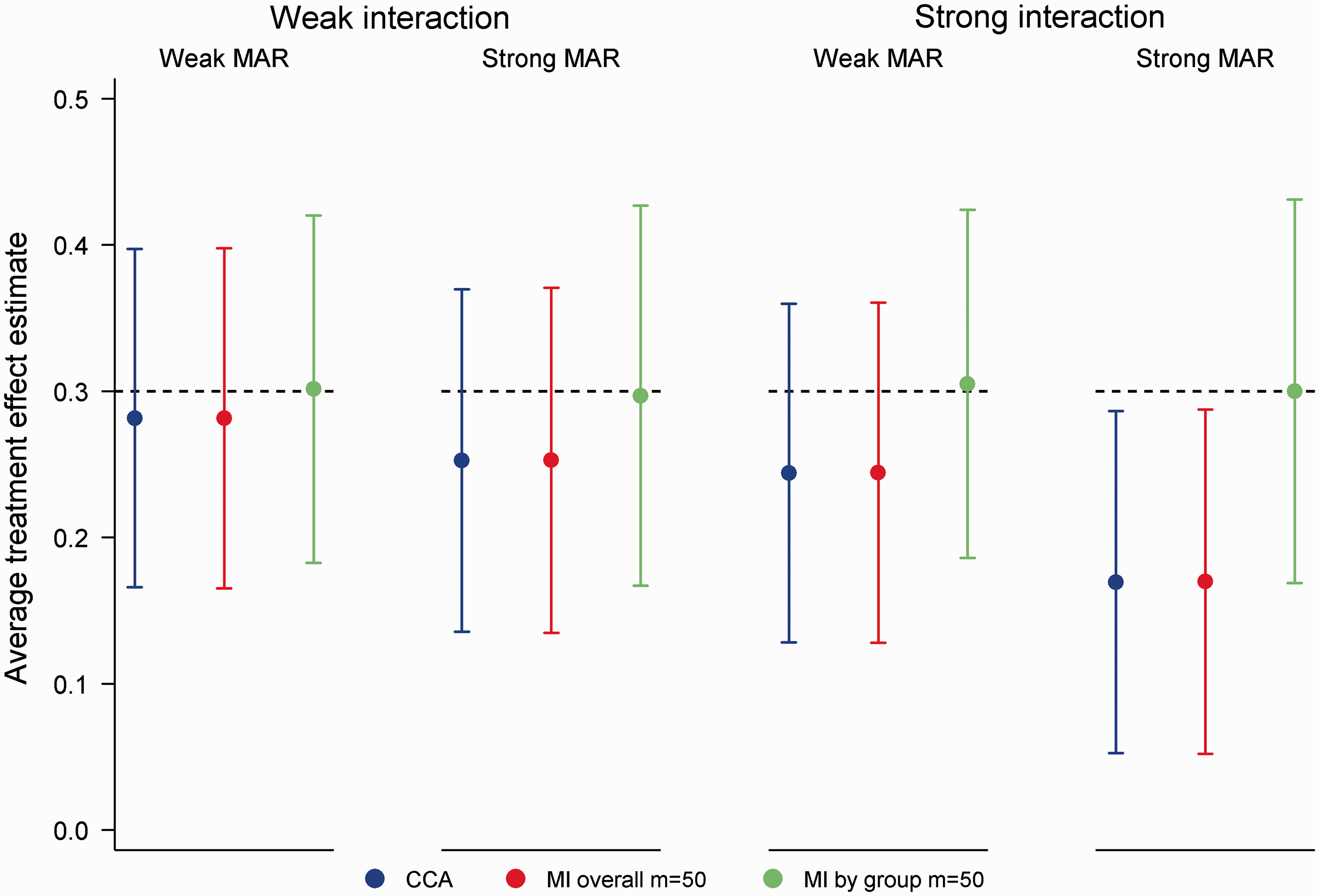

4.3 Misspecified analysis model, binary outcome

For binary outcomes, the notion of an ATE from a misspecified logistic regression model is more complex. Assuming effect modification by discrete X, omission of the interaction effect from the analysis model can lead to an ATE estimate that differs substantially from a weighted average of stratum specific effects (on both odds and log odds scales). In this setting, we consider the ATE that would have been observed with complete data as the ‘least false' ATE. In the presence of missing data, we assume the goal is to reproduce this least false ATE.

Considering binary X with $π_{0} = π_{1} = 0.5,$ data were generated from the model $logit P (Y_{i} = 1) = - 1.77 + β_{1} T_{i} + 0.69 X_{i} + β_{3} X_{i} T_{i}$ . The intercept value was chosen so that $P (Y = 1 | T = 0) = 0.20$ , while the coefficient for X gives $OR (Y, X | T = 0) = 2.0$ . Fixing the average of the stratum specific effects on the logit scale at 0.69 (OR = 2.0), we evaluated both weak ( $β_{1} = β_{3} = 0.46$ ) and strong ( $β_{1} = 0, β_{3} = 1.38$ ) interaction effects between X and T. Following generation of complete datasets, values in Y were set to missing according to the mechanisms described in Section 4.1.

Across the 24 simulation scenarios (12 missing data scenarios × 2 interactions), MI by group was unbiased in reproducing the least false ATE (absolute bias ≤ 0.02), with coverage remaining close to 0.95 (range 0.94, 0.96). In contrast, CCA and MI overall produced biased estimates under the MAR X and MAR X + T mechanisms. Figure 3 summarizes performance under the MAR X mechanism for 50% missing data. In parallel with results for continuous outcome data, the bias of CCA and MI overall increased with the strength of the missing data mechanism and the interaction between X and T.

Figure 3.

Mean average treatment effect estimates for 50% missing data in a binary outcome under the MAR X mechanism (odds of Y missing 1.5 (weak MAR) or 2.5 (strong MAR) times higher per standard deviation increase in X), incorrectly specified analysis model. Horizontal reference lines illustrate the least false average treatment effect in the absence of missing data. Error bars correspond to empirical standard errors (±1 standard error) across 2000 simulated datasets.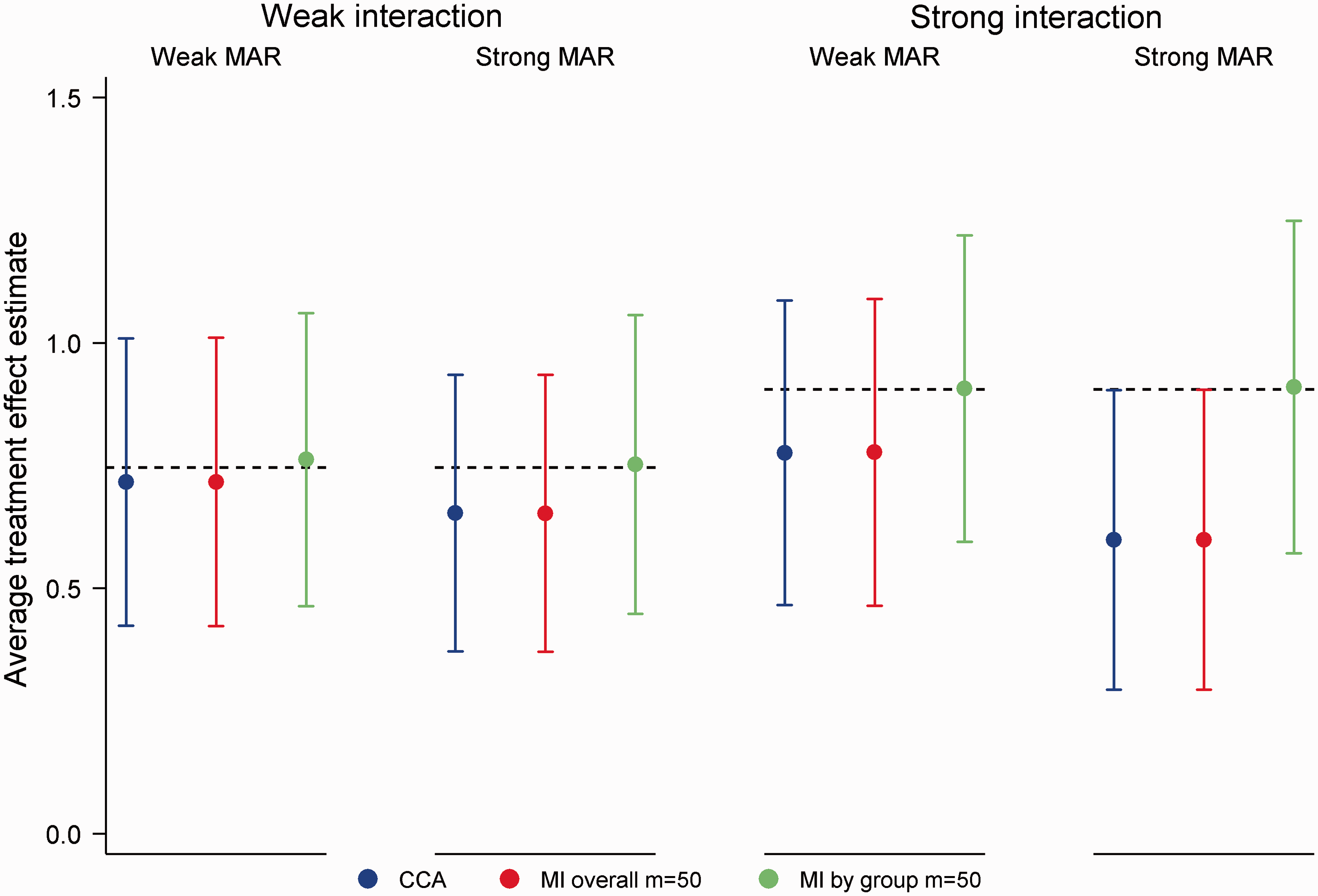

5 Missing data in a multivariate outcome and use of auxiliary variables

We now consider missing data in an outcome measured at repeated intervals following randomization, where interest concerns the effect of treatment at the final time point. Unlike the univariate case, the validity of CCA is questionable in this setting since it cannot incorporate information from intermediate measures of the outcome. Such measures may be associated with the probability of missing data and the value of the outcome at the final time point. By exploiting information in partially observed cases, MI and likelihood-based approaches have been favoured over CCA for the analysis of multivariate outcomes.^9,11,39,40 In what follows, we briefly introduce likelihood approaches for multivariate outcome data, describe the link between intermediate outcome measures and auxiliary variables, and present results from a simulation study comparing MI with alternatives.

Likelihood-based estimation of a linear mixed model (LMM)⁴¹ is a popular alternative to MI for handling missing data in a multivariate outcome. Based on the multivariate normal distribution, this approach incorporates all observed information on the repeated measures of the outcome to produce estimates that are valid under a MAR assumption. No explicit imputation is involved. For outcomes collected at a limited number of fixed time points following randomization, a LMM would typically include fixed effects for time (categorical), randomized group and the interaction between randomized group and time. Within-subject dependence due to repeated measurements is accounted for through specification of a covariance structure. Several authors have recommended the unstructured covariance matrix since it is easily pre-specified, entails minimal power loss compared with more parsimonious choices^9,42,43 and ensures that estimates are approximately equivalent to and slightly more efficient than those obtained from a comparable MI procedure.^9,14 With a single intermediate measure Z, a LMM with adjustment for X is

\begin{matrix} (\begin{matrix} Z_{i} \\ Y_{i} \end{matrix}) \sim N {(\begin{matrix} α_{0} + α_{1} T_{i} + α_{2} X_{i} \\ β_{0} + β_{1} T_{i} + β_{2} X_{i} \end{matrix}), (\begin{matrix} σ_{Z}^{2} & σ_{ZY} \\ σ_{ZY} & σ_{Y}^{2} \end{matrix})} \end{matrix}

(2)

In applying MI, the repeated measurements of the outcome are usually treated as distinct variables in the imputation model. Where interest lies in the treatment effect at the final time point, the analysis model need not include the intermediate outcome measures; following imputation a comparison of final time point results is sufficient.⁴⁴ In this case, the intermediate measures operate as auxiliary variables, assisting with the prediction of missing values at the final time point and making the MAR assumption more plausible. Other auxiliary variables, for instance measures of compliance or related outcomes, can also be added to the imputation model as required. If data are collected but more likely to be missing following treatment discontinuation, an indicator variable for discontinuation may also be valuable as an auxiliary variable. The ability to incorporate auxiliary variables, both for univariate and multivariate outcomes, is considered one of the key strengths of MI.⁴⁵ Less well known is that LMMs can also benefit from auxiliary variables through joint modelling with the outcome.^9,46 Using model (2) for illustration, Z could be an auxiliary variable rather than an intermediate outcome measure. By assuming an unstructured covariance matrix, multiple auxiliary variables are easily handled within a LMM.⁹

For the simulation study, intermediate (Z) and final $(Y)$ values of a continuous outcome were simulated from model (2) with $β_{0} = α_{0} = 0$ , $β_{1} = α_{1} = 0$ .30 and $σ_{Z}^{2} = σ_{Y}^{2} = 1$ . To evaluate whether the correlation between Z and Y impacted on model performance, we considered $σ_{ZY} = 0.30 or 0.70$ . We also examined both weak (0.30) and strong (0.70) correlations between X and the outcome measures. Following generation of complete datasets, values in Y were set to missing such that the odds of missingness were λ times higher per SD increase in Z (with λ = 1.5 or 2.5 and for 20% or 50% missing data). In addition to CCA and MI, data were analysed using a LMM with an unstructured covariance matrix. Treatment effect estimates for LMMs in this article were obtained using restricted maximum likelihood estimation with degrees of freedom calculated according to the Kenward–Roger method.⁴⁷

MI overall, MI by group and the LMM produced unbiased treatment effect estimates across the 16 simulation scenarios (4 missing data scenarios × 4 correlations), with coverage ≥ 0.94 throughout. Compared to the LMM, empirical SEs were on average 0.5% and 3.2% higher with MI overall and MI by group, respectively. The lost efficiency with MI by group was most noticeable in scenarios with 50% missing data and a strong MAR mechanism. Power was on average 0.3% lower for MI overall and 2.2% lower for MI by group compared to the LMM. By ignoring the intermediate measure of the outcome, CCA was, as expected, the least efficient approach. Although minimal in most settings, some bias was also evident with CCA. Figure 4 illustrates performance in scenarios with 50% missing data, a strong MAR mechanism and where $corr (X, Y | T) = 0.30$ . As seen in the figure, the relative performance of CCA was poor for $σ_{ZY} = 0.70$ (bias = 0.03, empirical SE 10.7% larger than the LMM). While outperforming CCA, MI offered no advantages over the LMM.

Figure 4.

Mean treatment effect estimates for 50% missing data in a continuous multivariate outcome, corr(X,Y|T) = 0.30, strong missing at random (MAR) mechanism. Error bars correspond to empirical standard errors (±1 standard error) across 2000 simulated datasets.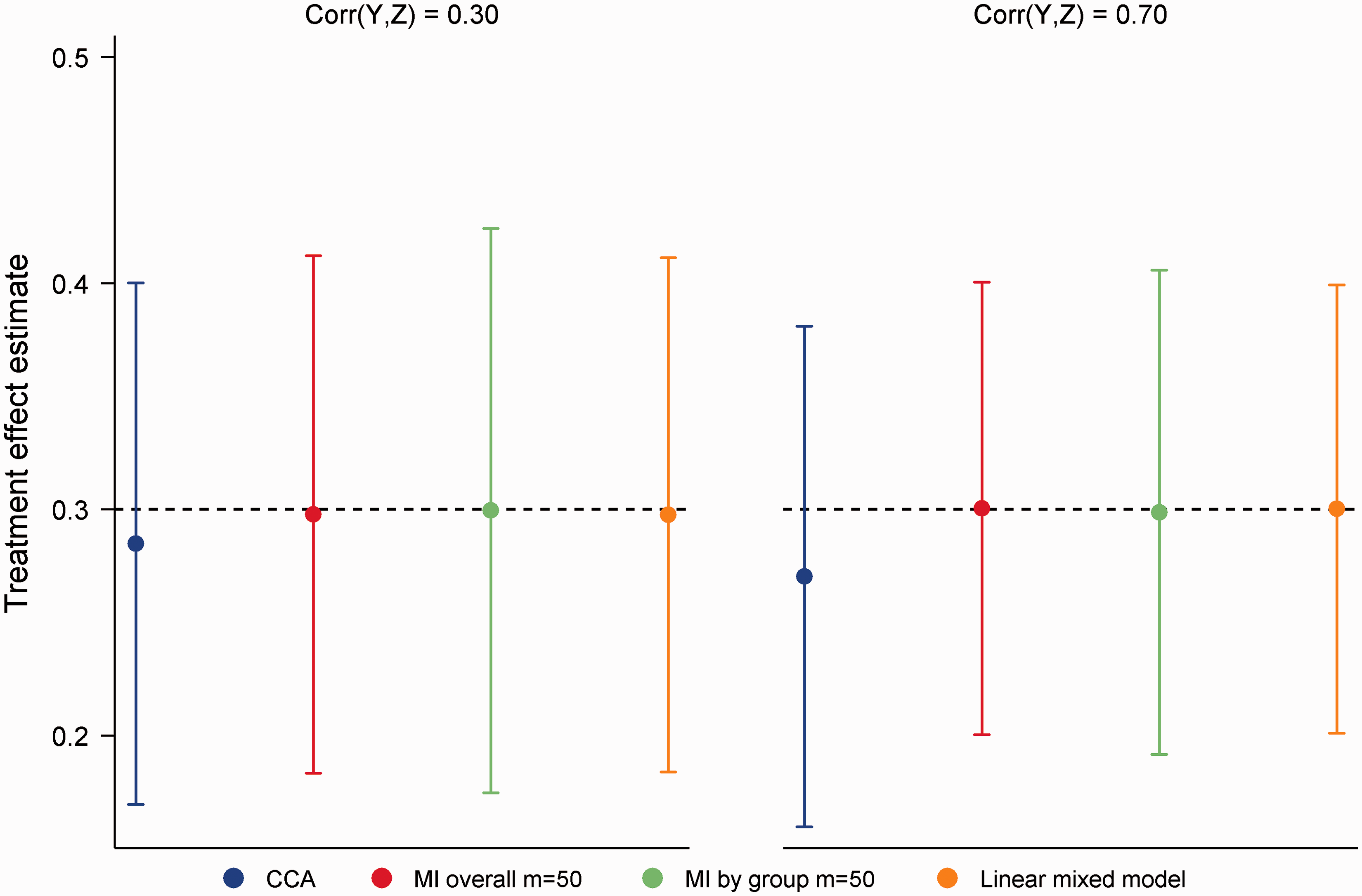

Similar results were obtained from a simulation study allowing missing data to occur in the intermediate as well as the final measure of the outcome, although the shortcomings of CCA were less pronounced in this setting (see online Appendix B). We did not consider a simulation study for binary multivariate outcome data due to complexities in defining the estimand (see Discussion).

6 Missing data in a baseline covariate

Although missing baseline data can be avoided by requiring complete data collection before randomization, this may not always be feasible (e.g. if a lengthy baseline interview is required). Unless baseline data are missing by design, it is implausible that missingness depends on randomized group given that baseline variables are measured before randomization.^9,48 In this context, group comparisons based on complete cases should be unbiased, even if baseline data are MNAR. One potential limitation of the standard implementation of MI for imputing missing baseline data is that it ignores the independence of X and T. Chance imbalances in X in the observed data are incorrectly extrapolated to the missing data, which may result in a loss of efficiency.⁴⁸ In this section, we evaluate the efficiency of MI using simulation, both for continuous and binary variables, and compare performance with alternative approaches.

6.1 Continuous baseline covariate and outcome

The binary indicator $M_{Xi}$ for missing data in the baseline covariate X was first simulated with a probability of 0.20. Unlike other scenarios, we did not consider 50% missing data, since this degree of missingness seems unlikely for a baseline covariate pre-specified for adjustment. Next, baseline and outcome data were simulated from the models $X_{i} = δ_{X} M_{Xi} + e_{1 i}$ and $Y_{i} = 0.30 T_{i} + β_{2} X_{i} + δ_{Y} M_{Xi} + e_{2 i}$ , with $e_{1} and e_{2} \sim N (0, 1)$ . The parameters $δ_{X}$ and $δ_{Y}$ in these models allow X and Y, respectively, to be associated with $M_{Xi}$ . Both MCAR ( $δ_{X} = δ_{Y} = 0$ ) and MNAR ( $δ_{X} = δ_{Y} = 0.30$ ) mechanisms were considered in separate simulation scenarios. In choosing values for $β_{2}$ , we allowed $corr (X, Y | T, M_{X} = 0)$ to range between 0.10 and 0.90 in increments of 0.20.

In addition to MI and CCA, we evaluated the performance of mean imputation, the missing indicator method and a LMM with baseline as an outcome. In mean imputation, missing baseline values are replaced with the mean of the observed values across both groups (i.e. $X_{i}^{*} = {\bar{X}}_{obs} if M_{Xi} = 1$ ). Although mean imputation for addressing missing outcome data has been widely criticized for failing to incorporate missing data uncertainty,^2,8 overstated precision is not a concern in this setting given the independence of X and T and interest only in the effect of treatment (and not the effect of the covariate).⁴⁸ The missing indicator method involves mean imputation and the addition of a dummy variable indicating missing data to the analysis model (i.e. adding $M_{Xi}$ ). Despite being inappropriate for general use,^49,50 the missing indicator method has been validated for addressing missing covariate data in RCTs, where X and T are independent and missingness in X is conditionally independent of Y.^48,51 For strong correlations between X and Y, White and Thompson⁴⁸ found that mean imputation and the missing indicator method became more efficient when participants with missing data were given a weight of $1 - corr (X, Y | T, M_{X} = 0)^{2}$ in the analysis (with observed cases retaining a weight of 1). We investigated both unweighted and weighted approaches. For the LMM, we considered a joint model for X and Y, where X was assumed to be independent of T, i.e.

\begin{matrix} (\begin{matrix} X_{i} \\ Y_{i} \end{matrix}) \sim N {(\begin{matrix} δ_{0} \\ β_{0} + β_{1} T_{i} \end{matrix}), (\begin{matrix} σ_{X}^{2} & σ_{XY} \\ σ_{XY} & σ_{Y}^{2} \end{matrix})} \end{matrix}

Under both MCAR and MNAR mechanisms, all methods produced unbiased treatment effect estimates with nominal coverage throughout (range 0.94, 0.96). Despite this, noticeable differences in efficiency were apparent across the different approaches to handling missing data. Figure 5 summarizes performance under the MCAR mechanism for $corr (X, Y | T, M_{X} = 0)$ = 0.10, 0.50 and 0.90. As seen in the figure, CCA was close to optimal for a strong correlation between X and Y but inefficient for weak to moderate correlations. Both mean imputation and the missing indicator method performed well, with weighting becoming important for strong correlations. MI was marginally less efficient than the weighted approaches and the LMM (empirical SEs on average 0.3% larger), with little difference seen between MI overall and MI by group. Lastly unadjusted CCA was highly inefficient for moderate to strong correlations between X and Y. Efficiency results under the MNAR mechanism closely mirrored those of the MCAR mechanism, with MI performing similarly to weighted mean imputation and the LMM across all values for $corr (X, Y | T, M_{X} = 0)$ (empirical SEs on average 0.3% larger with MI overall and MI by group than mean imputation and the LMM). Interestingly, the missing indicator method incorporating weights held a slight advantage over MI under the MNAR mechanism (empirical SEs on average 1.1% smaller than with MI), which can be attributed to inclusion of the prognostic variable M_X in the analysis model. A graphical summary of performance under the MNAR mechanism is shown in online Appendix C; we do not present results here given their similarity to the MCAR setting. Given the simplicity of alternative approaches to handling missing data in baseline covariates, there appears to be little reason to adopt MI in this setting.

Figure 5.

Mean treatment effect estimates for 20% missing data in a continuous baseline covariate, MCAR mechanism. Error bars correspond to empirical standard errors (±1 standard error) across 2000 simulated datasets.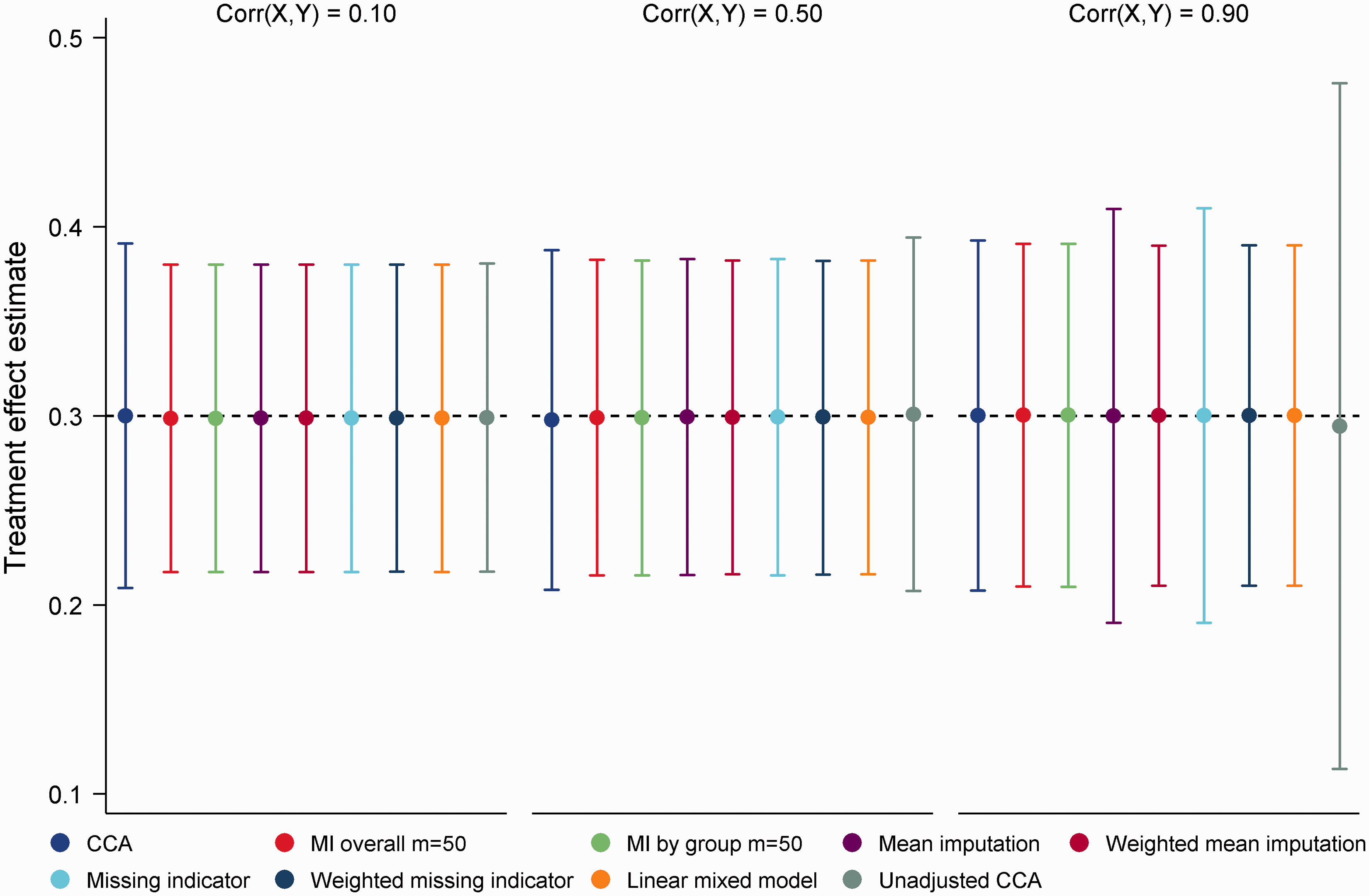

6.2 Binary baseline covariate and outcome

Following simulation of $M_{Xi}$ with probability 0.20, baseline and outcome data were generated from the models $logit P (X_{i} = 1) = δ_{X} M_{Xi}$ and $logit P (Y_{i} = 1) = β_{0} + 0.69 T_{i} + β_{2} X_{i} + δ_{Y} M_{Xi}$ . The coefficient $β_{2}$ was varied, so that $OR (Y, X | T, M_{X} = 0) =$ 2.0, 4.0 or 8.0, while $β_{0}$ was chosen to give $P (Y = 1 | T = 0, M_{X} = 0) = 0.20$ . Both MCAR ( $δ_{X} = δ_{Y} = 0$ ) and MNAR ( $δ_{X} = δ_{Y} = 0.69$ ) mechanisms were considered. We did not consider weighted methods or a LMM as in the continuous case, since these approaches are not applicable for binary outcomes.

Mean treatment effect estimates and empirical SEs for the MCAR mechanism are displayed in Figure 6. The clear outlier on these performance measures was unadjusted CCA. Since adjustment in logistic regression has the effect of increasing SEs and producing odds ratios that are further from the null,⁵² this finding is not surprising. Both MI overall and MI by group produced unbiased treatment effect estimates (absolute bias ≤ 0.004) with nominal coverage (range 0.95, 0.96) throughout, with little difference in empirical SEs between approaches. CCA produced treatment effect estimates with minimal bias, however empirical SEs were on average 10% larger than those of MI. For mean imputation and the missing indicator method, we observed a trade-off between efficiency and bias. For $OR (Y, X | T, M_{X} = 0) =$ 8.0, both approaches exhibited modest efficiency advantages over MI (empirical SEs 4% smaller) at the expense of a small bias (−0.02) towards the null. In terms of average power, there were minimal differences between mean imputation (93.0%), the missing indicator method (93.0%) and the MI approaches (92.9%). The small bias of mean imputation and the missing indicator arises because the methods estimate a treatment effect that lies between the marginal (unadjusted) and conditional (adjusted) estimands. As the proportion of missing data in X is increased, the methods shift from estimating the conditional estimand with no missing data to estimating the marginal estimand with no observed data (results not shown). Since for logistic regression the marginal estimand is always closer to the null, mean imputation and the missing indicator method produce estimates of the conditional treatment effect that are biased towards the null.

Figure 6.

Mean treatment effect estimates for 20% missing data in a binary baseline covariate, MCAR mechanism. OR (odds ratio) refers to OR(X,Y|T). Error bars correspond to empirical standard errors (±1 standard error) across 2000 simulated datasets.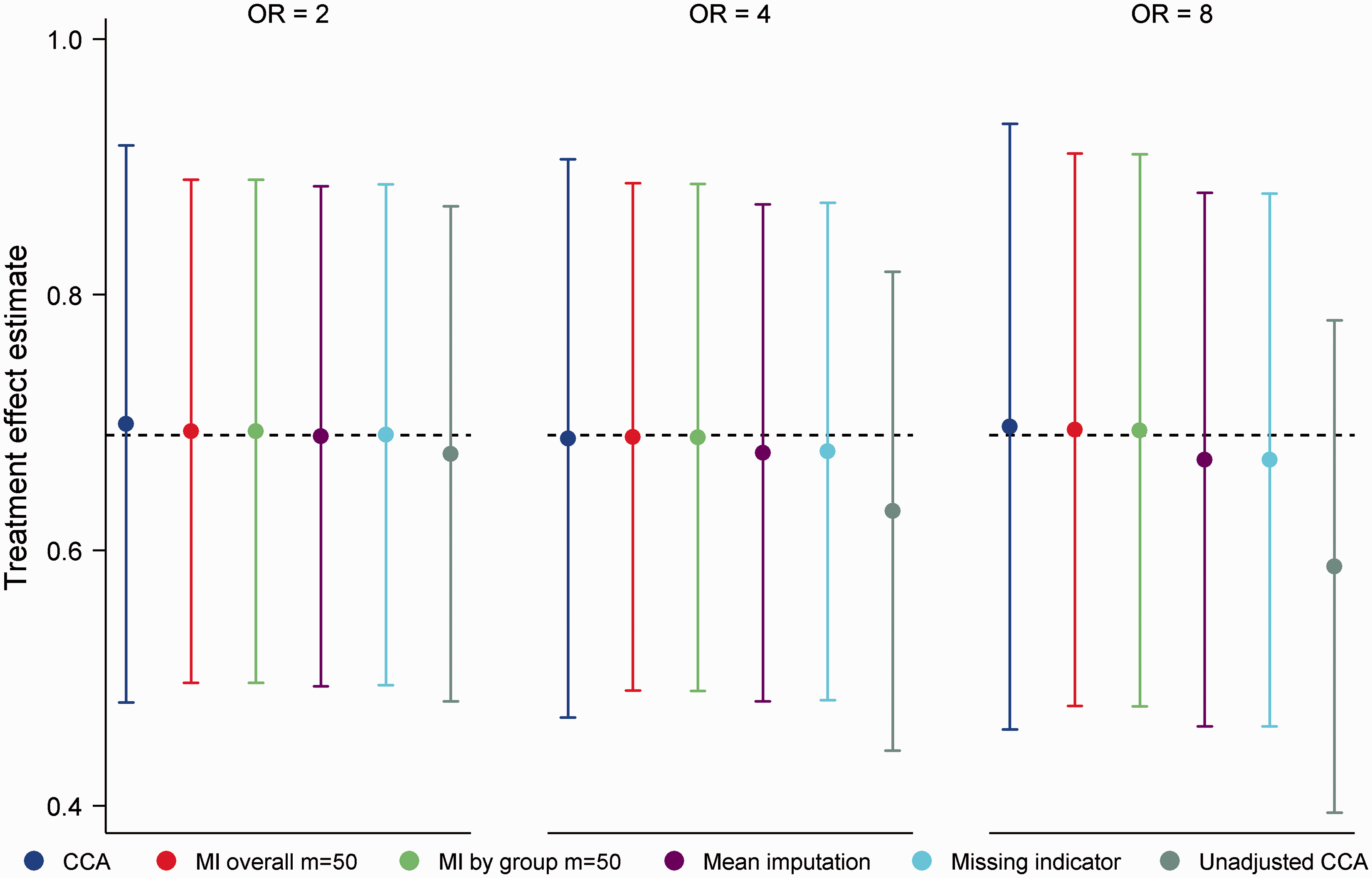

Although for $δ_{Y} \neq 0$ the omission of M_X from analysis models changes the treatment effect estimated by logistic regression, the observed changes were minimal across the MNAR scenarios considered. Based on complete data, the ‘least false' treatment effect from a misspecified model omitting M_X was approximately 0.68 for all values of $OR (Y, X | T, M_{X} = 0)$ . That distinction aside, results from the MNAR setting closely followed those of the MCAR setting (see Figure 7). In comparing MI with mean imputation, we once again observed a trade-off between efficiency and bias. For $OR (Y, X | T, M_{X} = 0) = 8.0$ , the empirical SE of mean imputation was 4.7% smaller than MI; however, the bias was slightly more pronounced (−0.05 vs. −0.02). The missing indicator method performed similarly to mean imputation in terms of efficiency, however biases were smaller in magnitude with the missing indicator method due to correct specification of the analysis model. Excluding unadjusted CCA, all methods produced treatment effect estimates with correct coverage (range 0.94, 0.95).

Figure 7.

Mean treatment effect estimates for 20% missing data in a binary baseline covariate, MNAR mechanism. OR (odds ratio) refers to OR(X,Y|T). Error bars correspond to empirical standard errors (±1 standard error) across 2000 simulated datasets.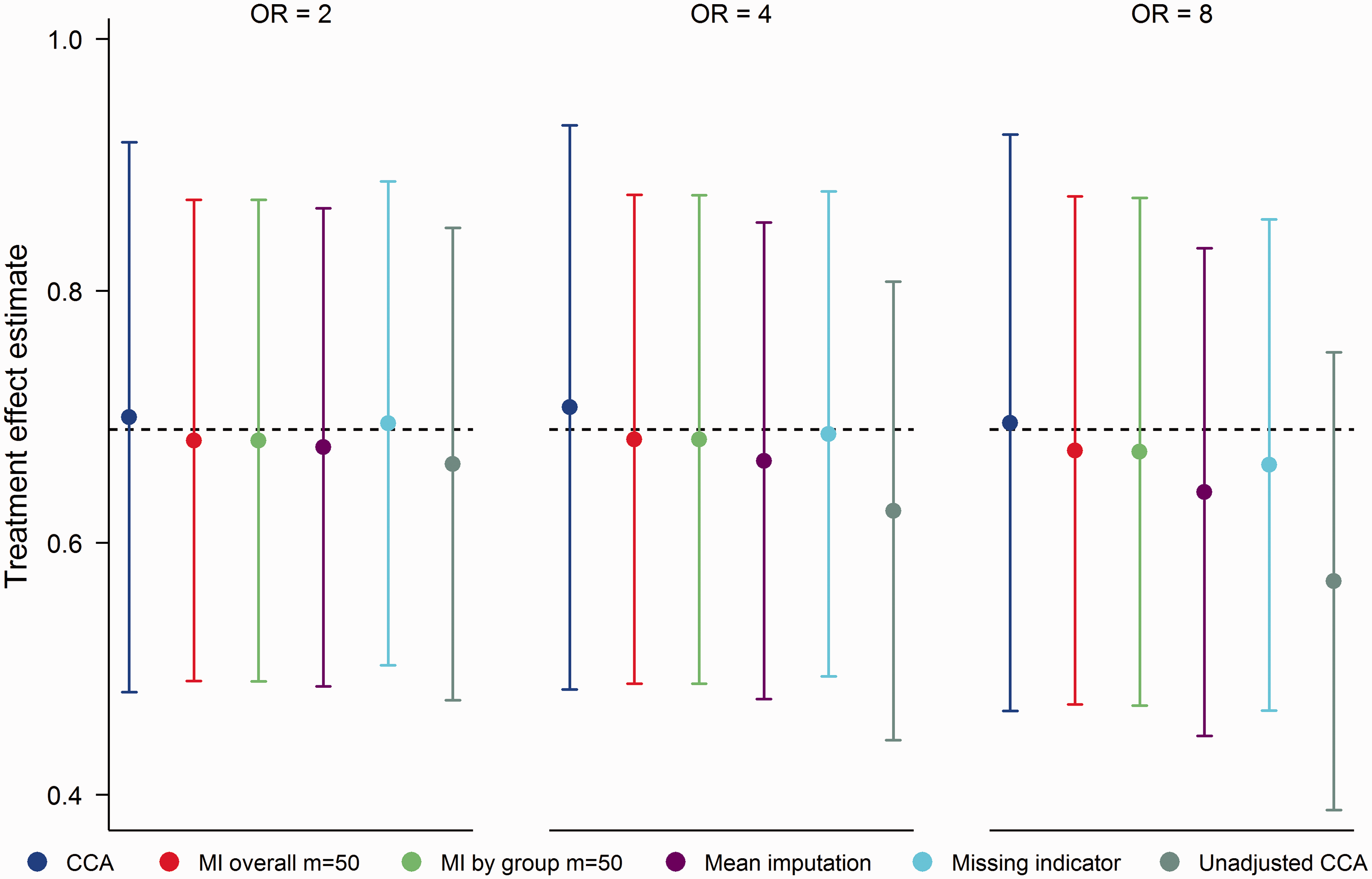

7 Case study

The Docosahexaenoic Acid for the Improvement of Neurodevelopmental Outcome in Preterm Infants (DINO) trial was a blinded RCT conducted in five Australian hospitals between 2001 and 2007 (Australian New Zealand Clinical Trials Registry: ACTRN12606000327583). Preterm infants born <33 weeks gestation (n = 657) were randomized to receive a high docosahexaenoic acid (DHA) or a standard DHA diet from within 5 days of commencing enteral feeds through to term. Randomization was stratified by hospital, sex and birth weight (<1250 g, ≥1250 g), with infants from a multiple birth randomized according to the sex and birth weight of the first born infant. Results for primary and key secondary outcomes have been published previously.^53–55 In the primary trial publication,⁵³ outcomes were re-analyzed using MI following feedback from reviewers that all randomized infants had to be included in ITT analyses and that MI would be an appropriate approach to achieve this. To simplify the dataset for illustration purposes, second and subsequent born infants from a multiple birth and infants that died before term were ignored, resulting in an example dataset with 262 and 260 infants in the high and standard DHA groups, respectively.

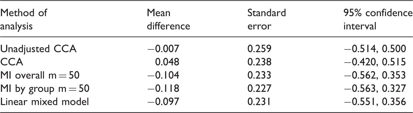
To illustrate approaches for handling missing outcome data, we consider comparisons of fat free mass (FFM) at 7 years corrected age. Excluding two children that died after term, FFM was missing for 65/262 (24.8%) and 46/258 (17.8%) children in the high and standard DHA groups, respectively. Logistic regression analysis revealed differences between the five study centres in the odds of missing outcome data (global p-value = 0.03). No other predictors of missing data were identified. For predictors of the outcome, linear regression analysis revealed associations between FFM and centre, sex and weight, height and systolic blood pressure at 7 years corrected age. Since centre and sex were baseline measures, for illustration purposes we imagine these variables were pre-specified as covariates for adjustment. Weight, height and systolic blood pressure at 7 years corrected age were treated as auxiliary variables.

We estimated the effect of treatment using CCA, MI overall, MI by group and a LMM. An unadjusted CCA was also conducted for comparison. Since the auxiliary variables contained missing data (approximately 10% for each variable), values were imputed using a Markov chain Monte Carlo algorithm assuming multivariate normality.¹⁴ Following a burn-in of 5000 iterations, m = 50 completed datasets were created. For the LMM, the three auxiliary variables and FFM were jointly modelled assuming an unstructured covariance matrix, with adjustment for centre and sex.

Treatment effect estimates are presented in Table 1. Although there was little evidence for an effect of treatment on FFM, subtle differences between the approaches are apparent. As expected, adjustment for prognostic baseline covariates in a CCA reduced the SE of the treatment effect estimate compared with the unadjusted analysis. By incorporating information from auxiliary variables, additional efficiency gains were evident for MI and the LMM, with similar estimates from the two approaches (as expected). However gains were small, perhaps because 48% of the children with a missing FFM value also had missing data on the three auxiliary variables. Even when fully observed, auxiliary variables may only have a meaningful impact on estimation when strongly correlated with the outcome.^45,56,57

Table 1.

Treatment effect estimates for fat free mass (kg) at 7 years corrected age from the Docosahexaenoic Acid for the Improvement of Neurodevelopmental Outcome in Preterm Infants trial.

Method of analysis	Mean difference	Standard error	95% confidence interval
Unadjusted CCA	−0.007	0.259	−0.514, 0.500
CCA	0.048	0.238	−0.420, 0.515
MI overall m = 50	−0.104	0.233	−0.562, 0.353
MI by group m = 50	−0.118	0.227	−0.563, 0.327
Linear mixed model	−0.097	0.231	−0.551, 0.356

For missing data in a baseline covariate, we consider group comparisons of head circumference (HC) at term adjusted for birth HC. To focus on the problem of missing baseline data, 20 infants with missing outcome data were excluded from the analysis. Seven of these infants were missing birth HC and hence contained no information for estimating treatment effects, while the remaining 13 were assumed to be MAR and hence could be validly excluded (as demonstrated in Section 4). Of the remaining infants, birth HC was missing for 39/251 (15.5%) and 42/251 (16.7%) in the high and standard DHA groups, respectively. Treatment effects were estimated using the same methods as in Section 6.1, with 50 imputations used for MI. In relation to the calculation of weights for mean imputation and the missing indicator method, in complete cases, the correlation between birth HC and HC at term was 0.43.

As illustrated in Table 2, estimates were similar across the nine statistical approaches. In line with simulation results for a moderate correlation between the baseline and outcome measure, CCA and unadjusted CCA produced the largest SEs for the effect of treatment. While outperforming CCA, MI did not offer any efficiency improvements over the remaining approaches.

Table 2.

Treatment effect estimates for head circumference (cm) at term from the Docosahexaenoic Acid for the Improvement of Neurodevelopmental Outcome in Preterm Infants trial.

Method of analysis	Mean difference	Standard error	95% confidence interval
Unadjusted CCA	−0.060	0.136	−0.326, 0.206
CCA	−0.058	0.134	−0.320, 0.204
MI overall m = 50	−0.023	0.125	−0.267, 0.221
MI by group m = 50	−0.027	0.125	−0.273, 0.218
Mean imputation	−0.024	0.125	−0.269, 0.221
Mean imputation with weights	−0.029	0.125	−0.274, 0.215
Missing indicator	−0.028	0.125	−0.272, 0.217
Missing indicator with weights	−0.032	0.124	−0.276, 0.211
Linear mixed model	−0.029	0.125	−0.275, 0.217

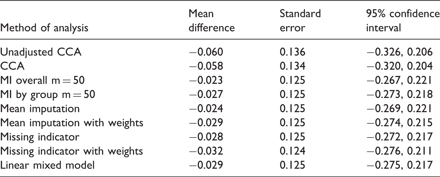
Since the probability of missing baseline data differed across the five study centres, we considered additional sensitivity analyses where centre was added as a covariate in adjusted models and mean imputation was performed separately by centre. Although this resulted in small increases in precision compared to models ignoring centre, again MI did not outperform simpler approaches such as mean imputation and the missing indicator method with or without weights (SE = 0.123 for all approaches).

8 Discussion

In this article, we evaluated the performance of MI in the RCT setting. In line with theoretical results, in its standard implementation, MI produced unbiased treatment effect estimates when data were MAR and the analysis model was correctly specified. However, due to Monte Carlo simulation error, MI was often less efficient than alternative unbiased approaches. For missing outcome data, MI was less efficient than CCA for univariate outcomes and the LMM for multivariate outcomes. For missing data in a baseline covariate, MI failed to outperform methods such as mean imputation and the missing indicator method. As well as being less efficient, MI was generally more difficult to implement and took longer to run compared with alternatives. Being a stochastic analysis, it also had the disadvantage of not producing a unique treatment effect estimate. Given these limitations, we believe that MI should not be seen as the only acceptable way to address missing data in RCTs.

Collectively, our results underline the importance of context in choosing an approach for handling missing data. While MI is an extremely useful general purpose tool, it appears most beneficial in observational settings when there are missing data in confounding variables.⁵⁸ In RCTs, some of the value of MI is lost, and other approaches that are not widely recommended can be employed. For example, our simulation results confirm that mean imputation and the missing indicator method, whose use is ill-advised in most settings,^2,8,49,50 can be validly applied for addressing missing covariate data in RCTs. Similarly, despite general recommendations against the use of CCA,^2,8 it is optimal when missing data are restricted to a univariate outcome and variables associated with missingness are included as covariates in the analysis model.^34–36 This scenario seems most pertinent to RCTs, where missing data tend to occur in the outcome. Of course should post-randomization auxiliary variables for a univariate outcome be available, as is often the case, we then move into the setting of multivariate data and approaches such as MI or a LMM should be preferred over CCA.

Regarding choice of imputation strategy, we found that MI by group was slightly less efficient than MI overall for a correctly specified analysis model. However, when the analysis model overlooked an interaction effect involving randomized group, only MI by group produced unbiased estimates of the ATE. Thus in settings where MI is adopted, we recommend imputing by randomized group; compared to MI overall, this approach offers greater robustness at little cost. The approach is also consistent with general recommendations for over- rather than under-specifying imputation models.^14,45 It should be noted that imputing by group only protects against bias in estimating the ATE if effect modifiers are included in the imputation model. Another possibility is to include interaction terms in a single imputation model, but this approach is more complex and may not be obvious when analysis models do not include interaction terms. Although not considered in this article, we agree with previous recommendations for performing imputation separately by randomized group in settings involving subgroup analyses.^11,20–22

Despite highlighting alternatives to MI in this article, we are not suggesting that it is inappropriate to use MI. To the contrary, we view MI as an attractive option given its considerable flexibility. It is not uncommon in RCTs for researchers to collect data on a large number of secondary outcomes. One of the strengths of MI is its ability to easily incorporate variables of different types (e.g. continuous, binary) in the imputation model, whether for univariate or multivariate data. An added benefit of including all outcomes in a single imputation model is that associations between related outcomes can aid imputation. Another appealing feature of MI is its ability to be implemented under an assumption that data are MNAR. This property makes MI well suited to undertaking sensitivity analyses around a primary assumption that data are MAR,⁵⁹ and as a primary method of analysis in settings where data are believed to be MNAR. One such setting is RCTs where participants cannot followed up after discontinuing treatment. If all observed data are ‘on-treatment’, a MAR assumption entails estimating the effect of treatment had all participants remained on their assigned treatment.²⁷ However, for a de facto type estimand (such as ITT), it may be more appropriate to assume that data are MNAR. In this situation, reference-based sensitivity analyses have been proposed, which at present require the use of MI.²³

A limitation of the current study is that conclusions were based on a restricted set of simulation scenarios. Although we only considered simple randomization to two groups, we anticipate that findings would extend to RCTs involving three or more randomized groups, unequal allocation probabilities and randomization using stratified blocks or minimization. We also expect that our results for normally distributed and binary outcome variables would apply to most other outcome types. Three exceptions worth noting are time to event outcomes, where missing outcome data can be addressed via censoring, composite (scale) outcomes derived from multiple items and binary multivariate outcomes. For missing data in a composite outcome, MI at the item level is a particularly convenient approach when the individual items are partially observed. Although likelihood-based alternatives for composite outcomes are also available,⁶⁰ they are more difficult to implement. For binary multivariate outcomes, complexities arise due to differences between population-averaged and subject-specific estimands.⁶¹ Generalized mixed models can be implemented in a similar manner to LMMs for continuous data if subject-specific estimates are of interest⁹; however, these models can be challenging to fit given the variety of estimation procedures available and the computational difficulties that can arise with large numbers of repeated measurements.⁶² MI is more appealing for producing population-averaged estimates.⁹

A further limitation is that we did not consider the performance of inverse probability weighting (IPW). This approach, which involves weighting complete cases by the inverse of the probability of being a complete case, requires only a correctly specified model for the probability of missing data to produce valid estimates under a MAR assumption. However, IPW tends to be less efficient than MI and can be difficult to implement for non-monotone missing data patterns.⁶³ Of relevance to the settings considered in this article, IPW is capable of producing population-averaged estimates for multivariate binary outcome data and unbiased estimates of an ATE from a misspecified analysis model.⁶³ IPW can also be appropriate in settings where data are missing by design and hence where the probability of being a complete case is known. We also did not evaluate multiple imputation then deletion, which is a modification to standard MI where participants with imputed outcomes (but not imputed covariate values) are deleted from analysis datasets.⁶⁴ The rationale behind this approach is that following imputation, participants with missing outcomes only contribute noise to the estimation procedure.⁶⁴ Whether MID is useful in the RCT setting is debatable however, since it is only applicable in settings where both covariate and outcome data are missing. Further, the approach should be avoided when auxiliary variables for the outcome are included in the imputation model,⁶⁵ as is often the case.

In summary, MI is not the only option for handling missing data in RCTs. Although MI is appropriate in all contexts, simpler alternatives are often slightly superior. For missing outcome data, MI can be inferior to CCA and likelihood-based approaches, adding in unnecessary simulation error. For missing data in a baseline covariate, simpler approaches such as mean imputation and the missing indicator method can outperform MI. Should MI be adopted, we recommend imputing separately by randomized group.

Footnotes

Declaration of conflicting interests

The author(s) declared no potential conflicts of interest with respect to the research, authorship, and/or publication of this article.

Funding

The author(s) disclosed receipt of the following financial support for the research, authorship, and/or publication of this article: T Sullivan was supported by an Australian Postgraduate Award. I White was funded by the Medical Research Council (Unit Programme number U105260558). K Lee was supported by a National Health and Medical Research Council Career Development Fellowship (1053609).

References

ICH E9 Expert Working Group. Statistical principles for clinical trials. International Conference on Harmonisation E9 Expert Working Group. Stat Med 1999; 18: 1905–1942.

Committee for Proprietary Medicinal Products. Guideline on missing data in confirmatory clinical trials, http://www.ema.europa.eu/docs/en_GB/document_library/Scientific_guideline/2010/09/WC500096793.pdf (2009).

Little

Cohen

Dickersin

et al.

The design and conduct of clinical trials to limit missing data. Stat Med 2012; 31: 3433–3443.

Fleming

. Addressing missing data in clinical trials. Ann Int Med 2011; 154: 113–117.

Bell

Fiero

Horton

et al.

Handling missing data in RCTs; a review of the top medical journals. BMC Med Res Methodol 2014; 14: 118–118. DOI: 10.1186/1471-2288-14-118.

Rubin

. Multiple imputation for nonresponse in surveys, New York: Wiley & Sons, 1987.

White

Carpenter

Horton

. Including all individuals is not enough: lessons for intention-to-treat analysis. Clin Trials 2012; 9: 396–407.

National Research Council, Panel on Handling Missing Data in Clinical Trials, Committee on National Statistics, Division of Behavioral and Social Sciences and Education. The prevention and treatment of missing data in clinical trials. Washington, DC: National Academies Press, 2010.

Carpenter

Kenward

. Missing data in randomised controlled trials - a practical guide, Birmingham: National Institute for Health Research, 2007.

10.

Molenberghs

Thijs

Jansen

et al.

Analyzing incomplete longitudinal clinical trial data. Biostatistics 2004; 5: 445–464.

11.

Bell

Fairclough

. Practical and statistical issues in missing data for longitudinal patient reported outcomes. Stat Methods Med Res 2014; 23: 440–459.

12.

Sterne

White

Carlin

et al.

Multiple imputation for missing data in epidemiological and clinical research: potential and pitfalls. Br Med J 2009; 338: b2393–b2393.

13.

Harel

Zhou

. Multiple imputation: review of theory, implementation and software. Stat Med 2007; 26: 3057–3077.

14.

Schafer

. Analysis of incomplete multivariate data, London: Chapman & Hall, 1997.

15.

Raghunathan

Lepkowski

Van Hoewyk

et al.

A multivariate technique for multiply imputing missing values using a sequence of regression models. Survey Methodol 2001; 27: 85–95.

16.

van Buuren

. Multiple imputation of discrete and continuous data by fully conditional specification. Stat Methods Med Res 2007; 16: 219–242.

17.

White

Royston

Wood

. Multiple imputation using chained equations: Issues and guidance for practice. Stat Med 2011; 30: 377–399.

18.

Hayati Rezvan

Lee

Simpson

. The rise of multiple imputation: a review of the reporting and implementation of the method in medical research. BMC Med Res Methodol 2015; 15: 30–30. DOI: 10.1186/s12874-015-0074-2.

19.

Mackinnon

. The use and reporting of multiple imputation in medical research - a review. J Int Med 2010; 268: 586–593.

20.

Schafer

Graham

. Missing data: our view of the state of the art. Psychol Methods 2002; 7: 147–177.

21.

Carpenter

Kenward

. Multiple imputation and its application, Chichester, UK: Wiley & Sons, 2013.

22.

Graham

. Missing data analysis: making it work in the real world. Annu Rev Psychol 2009; 60: 549–576.

23.

Carpenter

Roger

Kenward

. Analysis of longitudinal trials with protocol deviation: a framework for relevant, accessible assumptions, and inference via multiple imputation. J Biopharm Stat 2013; 23: 1352–1371.

24.

Permutt

. A taxonomy of estimands for regulatory clinical trials with discontinuations. Stat Med 2016; 35: 2865–2875.

25.

Heritier

Gebski

Keech

. Inclusion of patients in clinical trial analysis: the intention-to-treat principle. Med J Australia 2003; 179: 438–440.

26.

Moher

Hopewell

Schulz

et al.

CONSORT 2010 explanation and elaboration: updated guidelines for reporting parallel group randomised trials. Br Med J 2010; 340: c869–c869.

27.

Little

Kang

. Intention-to-treat analysis with treatment discontinuation and missing data in clinical trials. Stat Med 2015; 34: 2381–2390.

28.

Alshurafa

Briel

Akl

et al.

Inconsistent definitions for intention-to-treat in relation to missing outcome data: systematic review of the methods literature. PLoS One 2012; 7: e49163–e49163.

29.

Committee for Proprietary Medicinal Products. Points to consider on missing data, http://www.ema.europa.eu/docs/en_GB/document_library/Scientific_guideline/2009/09/WC500003641.pdf (2001).

30.

Altman

. Missing outcomes in randomized trials: addressing the dilemma. Open Med 2009; 3: e51–e53.

31.

Dziura

Post

Zhao

et al.

Strategies for dealing with missing data in clinical trials: from design to analysis. Yale J Biol Med 2013; 86: 343–358.

32.

Hernandez

Steyerberg

Habbema

. Covariate adjustment in randomized controlled trials with dichotomous outcomes increases statistical power and reduces sample size requirements. J Clin Epidemiol 2004; 57: 454–460.

33.

Kahan

Jairath

Dore

et al.

The risks and rewards of covariate adjustment in randomized trials: an assessment of 12 outcomes from 8 studies. Trials 2014; 15: 139–139. DOI: 10.1186/1745-6215-15-139.

34.

Little

RJA

. Regression with missing X’s: a review. J Am Stat Assoc 1992; 87: 1227–1237.

35.

Graham

Donaldson

. Evaluating interventions with differential attrition: the importance of nonresponse mechanisms and use of follow-up data. J Appl Psychol 1993; 78: 119–128.

36.

Groenwold

Donders

Roes

et al.

Dealing with missing outcome data in randomized trials and observational studies. Am J Epidemiol 2012; 175: 210–217.

37.

Chen

Ibrahim

. A note on the relationships between multiple imputation, maximum likelihood and fully Bayesian methods for missing responses in linear regression models. Stat Interf 2014; 6: 315–324.

38.

Snowden

Rose

Mortimer

. Implementation of G-computation on a simulated data set: demonstration of a causal inference technique. Am J Epidemiol 2011; 173: 731–738.

39.

Little

D’Agostino

Cohen

et al.

The prevention and treatment of missing data in clinical trials. New Engl J Med 2012; 367: 1355–1360.

40.

Beunckens

Molenberghs

Kenward

. Direct likelihood analysis versus simple forms of imputation for missing data in randomized clinical trials. Clin Trials 2005; 2: 379–386.

41.

Laird

Ware

. Random-effects models for longitudinal data. Biometrics 1982; 38: 963–974.

42.

Mallinckrodt

Clark

Carroll

et al.

Assessing response profiles from incomplete longitudinal clinical trial data under regulatory considerations. J Biopharm Stat 2003; 13: 179–190.

43.

Mehrotra

. Specification of covariance structure in longitudinal data analysis for randomized clinical trials. Stat Med 2010; 29: 474–488.

44.

Littell

Pendergast

Natarajan

. Modelling covariance structure in the analysis of repeated measures data. Stat Med 2000; 19: 1793–1819.

45.

Collins

Schafer

Kam

. A comparison of inclusive and restrictive strategies in modern missing data procedures. Psychol Methods 2001; 6: 330–351.

46.

Wang

Hall

. Correction of bias from non-random missing longitudinal data using auxiliary information. Stat Med 2010; 29: 671–679.

47.

Kenward

Roger

. Small sample inference for fixed effects from restricted maximum likelihood. Biometrics 1997; 53: 983–997.

48.

White

Thompson

. Adjusting for partially missing baseline measurements in randomized trials. Stat Med 2005; 24: 993–1007.

49.

Donders

van der Heijden

Stijnen

et al.

Review: a gentle introduction to imputation of missing values. J Clin Epidemiol 2006; 59: 1087–1091.

50.

Knol

Janssen

Donders

et al.

Unpredictable bias when using the missing indicator method or complete case analysis for missing confounder values: an empirical example. J Clin Epidemiol 2010; 63: 728–736.

51.

Groenwold

White

Donders

et al.

Missing covariate data in clinical research: when and when not to use the missing-indicator method for analysis. Canad Med Assoc J 2012; 184: 1265–1269.

52.

Hauck

Neuhaus

Kalbfleisch

et al.

A consequence of omitted covariates when estimating odds ratios. J Clin Epidemiol 1991; 44: 77–81.

53.

Makrides

Gibson

McPhee

et al.

Effect of DHA supplementation during pregnancy on maternal depression and neurodevelopment of young children: a randomized controlled trial. JAMA 2010; 304: 1675–1683.

54.

Collins

Makrides

Gibson

et al.

Pre- and post-term growth in pre-term infants supplemented with higher-dose DHA: a randomised controlled trial. Br J Nutr 2011; 105: 1635–1643.

55.

Collins

Gibson

Anderson

et al.

Neurodevelopmental outcomes at 7 years’ corrected age in preterm infants who were fed high-dose docosahexaenoic acid to term equivalent: a follow-up of a randomised controlled trial. BMJ Open 2015; 5: e007314–e007314.

56.

Graham

. Missing data: analysis and design, New York: Springer, 2012.

57.

Mustillo

. The effects of auxiliary variables on coefficient bias and efficiency in multiple imputation. Sociol Methods Res 2012; 41: 335–361.

58.

Lee

Carlin

. Recovery of information from multiple imputation: a simulation study. Emerg Themes Epidemiol 2012; 9: 3–3. DOI: 10.1186/1742-7622-9-3.

59.

Ratitch

O’Kelly

Tosiello

. Missing data in clinical trials: from clinical assumptions to statistical analysis using pattern mixture models. Pharm Stat 2013; 12: 337–347.

60.

Mazza

Enders

Ruehlman

. Addressing item-level missing data: a comparison of proration and full information maximum likelihood estimation. Multivar Behav Res 2015; 50: 504–519.

61.

Zeger

Liang

Albert

. Models for longitudinal data: a generalized estimating equation approach. Biometrics 1988; 44: 1049–1060.

62.

Bolker

Brooks

Clark

et al.

Generalized linear mixed models: a practical guide for ecology and evolution. Trends Ecol Evol 2009; 24: 127–135.

63.

Seaman

White

. Review of inverse probability weighting for dealing with missing data. Stat Methods Med Res 2013; 22: 278–295.

64.

Von Hippel

. Regression with missing Ys: An improved strategy for analyzing multiply imputed data. Sociol Methodol 2007; 37: 83–117.

65.

Sullivan

Salter

Ryan

et al.

Bias and precision of the “multiple imputation, then deletion” method for dealing with missing outcome data. Am J Epidemiol 2015; 182: 528–534.

Should multiple imputation be the method of choice for handling missing data in randomized trials?

Abstract

Keywords

1 Introduction

2 Intention to treat and missing data

3 Methods

3.1 Setting

3.2 MI

3.3 General simulation methods

4 Missing data in a univariate outcome

4.1 Correctly specified analysis model

4.2 Misspecified analysis model, continuous outcome

4.3 Misspecified analysis model, binary outcome

5 Missing data in a multivariate outcome and use of auxiliary variables

6 Missing data in a baseline covariate

6.1 Continuous baseline covariate and outcome

6.2 Binary baseline covariate and outcome

7 Case study

8 Discussion

Footnotes

Declaration of conflicting interests

Funding

References