
Abstract
Multivariate random-effects meta-analysis allows the joint synthesis of correlated results from multiple studies, for example, for multiple outcomes or multiple treatment groups. In a Bayesian univariate meta-analysis of one endpoint, the importance of specifying a sensible prior distribution for the between-study variance is well understood. However, in multivariate meta-analysis, there is little guidance about the choice of prior distributions for the variances or, crucially, the between-study correlation, ρB; for the latter, researchers often use a Uniform(−1,1) distribution assuming it is vague. In this paper, an extensive simulation study and a real illustrative example is used to examine the impact of various (realistically) vague prior distributions for ρB and the between-study variances within a Bayesian bivariate random-effects meta-analysis of two correlated treatment effects. A range of diverse scenarios are considered, including complete and missing data, to examine the impact of the prior distributions on posterior results (for treatment effect and between-study correlation), amount of borrowing of strength, and joint predictive distributions of treatment effectiveness in new studies. Two key recommendations are identified to improve the robustness of multivariate meta-analysis results. First, the routine use of a Uniform(−1,1) prior distribution for ρB should be avoided, if possible, as it is not necessarily vague. Instead, researchers should identify a sensible prior distribution, for example, by restricting values to be positive or negative as indicated by prior knowledge. Second, it remains critical to use sensible (e.g. empirically based) prior distributions for the between-study variances, as an inappropriate choice can adversely impact the posterior distribution for ρB, which may then adversely affect inferences such as joint predictive probabilities. These recommendations are especially important with a small number of studies and missing data.
Keywords
1 Introduction
The multivariate meta-analysis approach has been advocated to jointly synthesise multiple correlated results from related research studies.1,2 For example, in a meta-analysis of multiple outcomes, a cancer patient’s overall survival time is likely to be correlated with their progression-free survival time, and therefore, treatment effect estimates for both outcomes are likely correlated within a study. Similarly, in a network meta-analysis of multiple treatment groups, the treatment effect for A vs. B is likely correlated with that for A vs. C. Compared to separate univariate meta-analyses, the multivariate approach utilises such correlation to gain additional information toward the estimation of summary meta-analysis results.3,4 This is especially advantageous when there are missing effect estimates in some studies (such as missing direct comparisons in network meta-analysis) and when there is potential outcome reporting bias,5,6 as the correlation can lead to more precise inferences and/or a reduction in bias, 2 which has been referred to as ‘borrowing of strength’ 7 .
The Bayesian framework for multivariate meta-analysis is a natural way to account for all parameter uncertainty, to make predictions regarding the possible effects in new studies, and to derive joint probability estimates regarding the multiple effects of interest. However, it requires the specification of prior distributions for all unknown parameters, which may be considered a disadvantage when genuine prior information does not exist. A previous simulation study of Bayesian univariate meta-analyses 8 found that the pooled effect estimates can be particularly sensitive to the choice of prior distribution for the between-study variance, even when seemingly ‘vague’ prior distributions are specified. To address this, previous work has utilised a large collection of existing meta-analyses to generate empirical prior distributions for the unknown between-study variance in a new univariate meta-analysis of intervention effects for continuous outcomes 9 and binary outcomes,10,11 across a wide range of healthcare settings, such as where the outcome of interest is all-cause mortality.
In addition to prior distributions for the between-study variances, a multivariate meta-analysis also requires prior distribution(s) for the between-study correlation(s). One might address this using the conjugate prior distribution for the entire between-study variance-covariance matrix, which is the inverse-Wishart prior distribution, and this has been used by previous authors, such as bivariate meta-analyses of test accuracy studies.12–14 However, others argue that it is preferable to place separate prior distributions on each component of the between-study variance-covariance matrix because the Wishart prior distribution can be very influential toward the posterior estimates of the between-study variances;14–17 the Wishart distribution is a generalisation of the Gamma distribution, which is known to be influential in univariate meta-analysis when used as a prior distribution for the between-study variances, especially when the true between-study variances are close to zero. 8 Separation of the between-study variance-covariance matrix also allows more flexibility in the choice of prior distributions for each component, for instance if genuine prior information was available for some, but not all, of the components.
In situations where separate prior distributions are placed on the between-study variances and correlations, an unanswered question remains: what is the impact of the choice of prior distributions for the between-study correlations and variances in a multivariate meta-analysis, especially in situations where little or no prior information is available? Appropriate estimation of the between-study variance-covariance matrix is important to making valid inferences, and thus undesired influence of prior distributions is unwanted when prior information is unavailable. For instance, appropriate estimation of the between-study correlation is desired because it dictates the magnitude of the borrowing of strength 1 and is therefore potentially influential toward pooled effects, credible intervals and prediction intervals; it is also pivotal when estimating functions of the pooled estimates or when deriving joint probability estimates (such as the probability that the treatment is effective for all outcomes). However, in our experience, most previous Bayesian applications of multivariate meta-analysis (including some of our own) adopt a Uniform(−1,1) prior distribution for the between-study correlation but do not conduct sensitivity analyses to check whether it is appropriate or influential.1,17,18
The aim of this paper is to examine the impact of seemingly vague and realistically vague prior distributions for the between-study correlations and variances in a bivariate meta-analysis, to extend previous work in the univariate setting. 8 Real application and an extensive simulation study are described, focusing on a Bayesian bivariate meta-analysis of treatment effects for two correlated outcomes, and investigating how the choice of prior distributions impacts upon posterior estimates of the pooled treatment effects and between-study covariance matrix, the accuracy of 95% credible and prediction intervals, and joint probabilistic inferences. Both complete and missing outcome data situations are examined, and the impact on the amount of borrowing of strength (that is, the change in pooled results and credible intervals from univariate to bivariate analysis) is also considered.
The remainder of this paper is structured as follows. Section 2 introduces the bivariate random-effects meta-analysis model and potential prior distributions for the between-study variances and correlation. Section 3 describes the methods and results of the simulation study. The key findings are then illustrated in the context of a real meta-analysis dataset in Section 4. Section 5 concludes with some discussion and recommendations.
2 General model for bivariate random-effects meta-analysis
This section summarises the general framework for bivariate meta-analysis, and it introduces possible prior distributions for the between-study variances and correlation. We focus on the use of bivariate meta-analysis for two correlated outcomes, but the issues remain similarly pertinent in other situations of correlated effects, such as multiple treatment groups (network meta-analysis) and multiple performance statistics (such as sensitivity and specificity).19,20
2.1 Model specification
Suppose that each of i = 1 to n, studies examines an effect of interest (such as a treatment effect) for two outcomes (j = 1, 2), such as systolic and diastolic blood pressure, or overall and progression-free survival. Let each study provide the estimated effects, Yi1 and Yi2, and their associated standard errors, si1 and si2, where each Yij is an estimate of an underlying true value, θij, and these true values may vary between studies due to heterogeneity. Assuming the Yij and θij are drawn from a bivariate normal distribution, and that the within-study variance-covariance matrix (
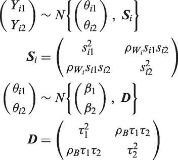
The true values (θij), therefore, have a mean value βj (referred to as the ‘pooled’ effect for outcome j) and between-study variance, τj2. The within-study covariance matrix,
2.1.1 Within-study and between-study correlation
Within-study and between-study correlation are two measures of correlation in a multivariate random-effects meta-analysis model. The within-study correlation is a measure of the association between the effect estimates in each study and is caused by the same patients contributing correlated data toward both outcomes. Estimation of model (1) typically assumes that these are known (just as the within-study variances are assumed known), 1 and for the purposes of this paper, we also make this assumption. Authors such as Riley et al. 23 and Trikalinos et al. 24 detail how to derive within-study correlations when individual participant data are available, but these can also be approximated using aggregate data in some other situations. 25 Alternatively, it is possible to construct prior distributions from previous studies.21,22
The between-study correlation is a measure of how the true underlying effects are related across studies and occurs because of between-study heterogeneity in, for example, the dosage of a drug or patient characteristics of the study populations, such as age. The between-study correlation is unknown and must be estimated in the meta-analysis model, alongside the between-study variances.
Both within- and between-study correlation can influence the amount of borrowing of strength in a bivariate meta-analysis.5,7 Within-study correlations are more influential when the within-study variances are large relative to the between-study variance, whereas the between-study correlation is more influential when the between-study variances are large relative to the within-study variances. Furthermore, accounting for such correlation is essential when an aim is to make joint inferences about the two effects of interest, such as the probability that they are both above a particular value.
2.2 Model estimation
In a frequentist framework, model (1) can be estimated by methods of moments or restricted maximum likelihood. 2 Within a Bayesian framework, the likelihood pertaining to model (1) is combined with prior distributions for the unknown parameters of βj, τj2, and ρB, and then posterior inferences are derived by sampling from the marginal posterior distributions using, for example, Markov chain Monte Carlo (MCMC) via Gibbs sampling. The convergence of parameters must be checked, which can be done visually using history and trace plots, and possible autocorrelation must be examined, which can be reduced by thinning the samples.
The prior distributions for the pooled effects (βj) are not evaluated and are given a vague N(0, 10002) prior distribution throughout. Here, the focus is on examining different choices of the prior distributions for τj 2 and, especially, ρB, and these are now discussed.
2.3 Choice of prior distribution for τj
In univariate meta-analysis, the prior distribution for 1/τ2 was once commonly chosen to be the Gamma(ε, ε) distribution with the misperception that if ε were very small (i.e. 0.001), then this distribution would be ‘vague’ 8 . However, previous work by Lambert et al. 8 (and more generally outside the meta-analysis field by Gelman 26 ) demonstrated that the Gamma distribution is not appropriate, as posterior inferences for the between-study variance and pooled effects are sensitive to ε. Here, ε must be set to a reasonable value, or meta-analysts should rather use one of a number of different weakly informative prior distributions discussed by Lambert et al. 8 and Gelman. 26 These refer to distributions that are set up so that the information they provide is weak but contain only realistic values for the variance. These include the half-Normal (0,a) distribution,27,28 and the half-t family of distributions, such as the half-Cauchy distribution. 26 In particular, for the half-Normal (0,a) distribution, the value of a can be chosen to cover all realistic values of the between-study variance, for example, as identified from other previous meta-analyses of the same outcome type in the same disease field.
The latter idea leads naturally to empirically based prior distributions for the between-study variances. 29 Indeed, previous work has used a large collection of existing meta-analyses to generate empirical prior distributions for the unknown between-study variance in a new univariate meta-analysis of intervention effects for continuous outcomes 9 and binary outcomes,10,11 across a wide range of healthcare settings, such as where the outcome of interest is all-cause mortality.
Here, in the setting of bivariate meta-analysis, we interrogate some inappropriate and sensible/weakly informative prior distributions for the between-study variances, to explore their impact on bivariate meta-analysis estimates and conclusions. In particular, in the simulation study (Section 3), two contrasting prior distributions for the between-study variances are compared: an inappropriate Gamma distribution and a more suitable truncated normal distribution that was suggested by Lambert et al. 8 Then, in the illustrative example in Section 4, a relevant empirical prior distribution is chosen and compared to an inappropriate Gamma prior distribution.
We include an inappropriate Gamma distribution for 1/τ2 in both simulations, and the example to highlight the danger of using this (or its extension, the Wishart distribution) as a prior distribution for the between-study variances in the context of bivariate meta-analysis applications, with particular emphasis on how it can adversely affect the posterior distribution for ρB, and the amount of borrowing of strength toward the pooled effects. Although it is well documented that inverse-Gamma and Wishart prior distributions for variance terms are inappropriate, unfortunately, they are still adopted in the meta-analysis field. For example, Menke, 30 Riley et al., 12 and Zwinderman and Bussuyt 13 use a Wishart prior distribution in bivariate meta-analyses of sensitivity and specificity from multiple test accuracy studies. Yang et al. 31 use a Wishart prior distribution in their network meta-analysis of multiple therapies for acute ischemic stroke, as does Jansen 32 in a network meta-analysis of multiple treatments of lung cancer. In their seminal paper on the Bayesian approach to multivariate meta-analysis of multiple outcomes, Nam et al. 18 use an inverse Gamma prior on each of the between-study variances. Therefore, given its continued use, herein it is important to demonstrate the drawback of the Gamma prior distribution within multivariate meta-analysis, with a novel angle on its impact on ρB, the amount of borrowing of strength and joint inferences.
2.4 Choice of prior distribution for ρB
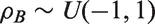
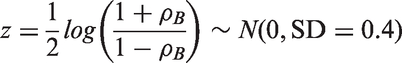
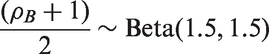
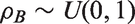
A range of (realistically) vague prior distributions for the between-study correlation are considered to account for varying levels of hypothetical prior knowledge. Below are five possible prior distributions in which options 1 to 3 allow the between-study correlation to be positive or negative, and options 4 and 5 only allow the between-study correlation to be positive. The five prior distributions are shown in Figure 1.
Density plots for prior distributions for between-study correlation: (a) ρB∼Uniform(−1,1) (option 1); (b) 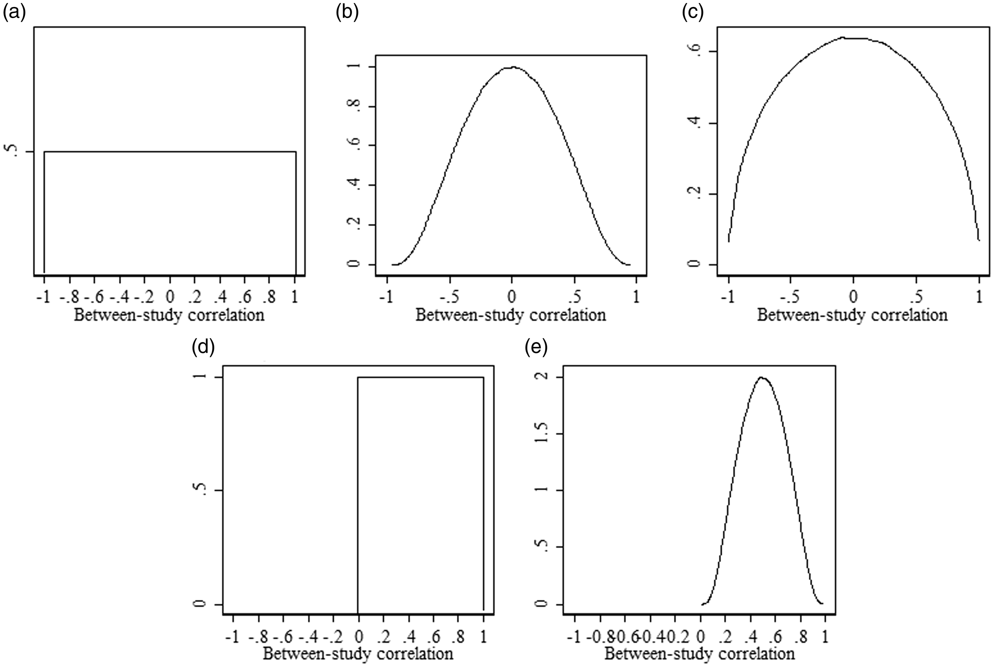
Option 1
Option 2
Option 3
Option 4
Option 5

Although these five prior distributions reflect a key range of options, we recognise that other choices of prior distributions could be specified. In particular, it may be that negative values of the correlation are very unlikely but not impossible and therefore a prior distribution might be specified that, unlike priors 4 and 5, allows for some small probability of negative values. An example of such a prior distribution is shown in the Supplementary Material. Clearly, the choice will be context specific but here onwards the five prior distributions described above are our key focus.
3 Simulation study to examine choice of prior distributions
We now describe the methods and results of the simulation study to examine the impact of (realistically) vague prior distributions for the between-study variances and correlation in a Bayesian estimation of bivariate meta-analysis model (1). The simulation focuses mainly on N = 10 studies per meta-analysis, but both complete data (both outcomes available in all 10 studies) and missing data (some studies only provide one outcome) situations are considered. Alternative N is also considered briefly in Section 3.2.5.
3.1 Methods of the simulation study
The simulation study involves three key steps, as follows.
Step 1: Generation of bivariate meta-analysis datasets for a range of settings
Settings for which simulated meta-analysis datasets were generated.
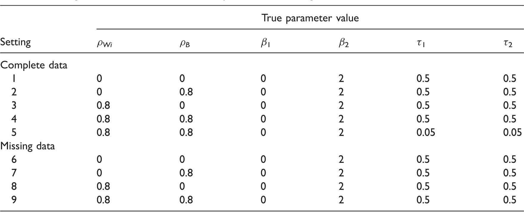
Within-study variances (sij 2 ) were drawn from a log normal distribution and had an average value of 0.5. Therefore, settings 1 to 4 and 6 to 9 had similarly sized within- and between-study variances on average, whilst settings 5 and 10 had relatively large within-study variances.
Settings 1 to 5 involve complete data (i.e. Yi1 and Yi2 are available for all studies) but settings 6 to 9 involve missing data, where some studies were made to have only Yi2. Missing data scenarios are very important, as borrowing of strength may be large in such situations. We chose to generate non-ignorable missingness. In each complete data meta-analysis dataset, the treatment effect estimate for outcome 1 (Yi1) was selectively removed if it was larger than the unweighted mean of Yi1 within each set of 10 trials, i.e.
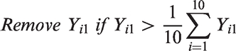
On average, this process removed half of the treatment effect estimates and their standard deviations (SD) for outcome 1 in the simulated datasets. This missing data process was chosen to reflect selective outcome reporting bias in which an outcome is measured and analyzed but not reported on the basis of the results.34,35 Although this missing data mechanism is missing-not-at-random, the utilisation of correlation from reported outcomes can still reduce (though not entirely remove) bias in univariate meta-analysis results in this situation, as shown elsewhere, 6 and is now a key reason for applying the multivariate model. 36 Therefore, it is of particular interest whether chosen prior distributions affect the bivariate meta-analysis results for outcome 1 in this setting.
Step 2: Fit model (1) to each dataset in each setting, for all the different sets of prior distributions
To each of the 1000 meta-analysis datasets within each of the nine settings, model (1) was fitted using MCMC with a particular set of chosen prior distributions. This was then repeated for each different set of prior distributions. The different sets of prior distributions were as follows.
Pooled effects (βj)
The prior distributions for βj were always given a vague N(0, 10002).
Between-study variances (τj 2 )
Two prior distributions for τj 2 were chosen (one that appeared appropriate and one that appeared inappropriate) based on the results of a univariate meta-analysis of the simulated datasets where ρWi = ρB = 0 in model (1) (see Table S1 in the Supplementary material). Because the true between-study SD in the simulations were 0.5, a τj∼N(0,2) (τj > 0) prior distribution appeared most suitable (realistically vague) among six prior distributions previously explored by Lambert et al. 8 In contrast, the Gamma(0.1,0.1) prior distribution for 1/τj 2 was, as expected, by far the poorest in terms of estimating τj accurately. However, as this inappropriate prior distribution is still often adopted in the multivariate meta-analysis literature (see earlier), we include it here to highlight its impact. Thus, in each setting of the simulation study, both these prior distributions were evaluated to compare the impact of a seemingly suitable prior distribution with a seemingly inappropriate prior distribution for τj.
Between-study correlation (ρB)
The prior distributions evaluated for ρB were the five prior distributions detailed in Section 2.4.
All combinations of prior distributions for between-study correlation and between-study variance.
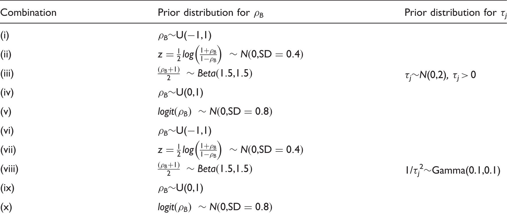
U: Uniform.
In each analysis, the posterior parameter estimates were obtained using the Gibbs Sampler MCMC method, which was implemented in SAS 9.3 using the PROC MCMC procedure. 37 For each dataset, the analyses were performed with 300,000 iterations after allowing for a 200,000 iteration burn in and the samples were thinned by 100 to reduce autocorrelation (see Supplementary Material for SAS code). The convergence of parameters was checked using history and trace plots.
Step 3: Summarise results
In each setting, to summarise and compare the posterior results for each set of prior distributions, the following were calculated from the set of 1000:
The mean posterior mean of pooled effects across all simulations, the mean and median posterior median of between-study SD across all simulations, and the mean and median posterior median of between-study correlation across all simulations (to check for bias); The mean and median SD of the posterior pooled effects across simulations; The mean-squared error (MSE) of the pooled effects, calculated by the average squared difference from the true value across the 1000 simulated datasets; The coverage performance of the 95% credible intervals for the pooled effects, calculated by the percentage of the 1000 95% credible intervals that contain the true effect.
Furthermore, we also evaluated performance in terms of predictive inferences about treatment effects in new trials. The predictive distribution of treatment effects in a new trial was assumed to be

In each analysis, values of θi1
new
and θi2
new
were sampled from this distribution during the MCMC process, which naturally accounts for the uncertainty in the pooled average effects, β1 and β2, and the uncertainty in the between-study covariance matrix, The average marginal probability that θi1
new
> 0, the average marginal probability that θi2
new
> 2, and the average joint probability that both θi1
new
> 0 and θi2
new
> 2.
In settings 1, 3, 6, and 8, where ρB = 0, the two true marginal probabilities that θi1 new > 0 and θi2 new > 2 was both 0.5, and the true joint probability that θi1 new > 0 and θi2 new > 2 was 0.25. When ρB = 0.8 in settings 2, 4, 5, 7, and 9, the true joint probability was 0.4.
3.2 Results of the simulation study
3.2.1 Complete case data when using prior distribution for between-study variance of τj∼N(0,2) (τj > 0)
Simulation results for 10 studies with complete data (setting 1). The within-study correlation, ρWi was zero and the same for each study. The prior distribution for τj is N(0,2)I(0,) and for βj is N(0,10002).

MSE: mean-square error; CrI: credible interval; SD: standard deviation; U: Uniform.
The means and medians represent the posterior means and medians from the distribution of summary estimates from the 1000 datasets.
Simulation results for 10 studies with complete data (setting 4). The within-study correlation, ρWi was 0.8 and the same for each study. The prior distribution for τj is N(0,2)I(0) and for βj is N(0,10002).

MSE: mean-square error; CrI: credible interval; SD: standard deviation; U: Uniform.
The means and medians represent the posterior means and medians from the distribution of summary estimates from the 1000 datasets.
In all settings, the choice of prior distribution for ρB is informative of the posterior estimate of ρB. This is expected since there are only 10 studies per meta-analysis, so there are only 10 data points to estimate a correlation, and thus the posterior mean is similar to the prior mean. For example, in setting 1 (ρWi = ρB = 0, Table 3) where ρB∼Uniform(−1,1), the mean posterior median for ρB across simulations is 0.007. When ρB∼Uniform(0,1), the mean posterior median for ρB across simulations is 0.412. A similar result is observed in settings 2 to 4. In settings 2 and 4, the true value of ρB is 0.8; however, none of the selected prior distributions led to average medians of ρB across simulations close to its true value. For example, in setting 4 (ρWi = ρB = 0.8, Table 4) where ρB∼Uniform(0,1), the average posterior median of ρB is only 0.646.
The performance of the 95% credible intervals is also close to 95% for βj regardless of the choice of prior distribution for ρB. Furthermore, the choice of prior distribution for ρB has little impact on the posterior means of β1 and β2 across simulations, and their mean SD. In other words, there appears to be very little borrowing of strength, which agrees with previous work that shows the borrowing of strength in a bivariate meta-analysis toward the estimates of βj is usually very small when complete data are available for both outcomes.5,33
However, the prior distribution for ρB does have a larger impact upon average joint inferences across both outcomes. The average joint probability that
3.2.2 Complete case data when using prior distribution for between-study variance of 1/τj2∼Gamma(0.1,0.1)
Simulation results for 10 studies with complete data (setting 3). The within-study correlation, ρWi was 0.8 and the same for each study. The prior distribution for 1/τj 2 is Gamma(0.1,0.1) and for βj is N(0,10002).

MSE: mean-square error; CrI: credible interval; SD: standard deviation; U: Uniform.
The means and medians represent the posterior means and medians from the distribution of summary estimates from the 1000 datasets.
The posterior means for β1 and β2 remain approximately unbiased for all choices of the prior distributions for ρB, for settings 1 to 4. However, the posterior distributions of the τj 2 s are centred on much larger values than 0.25 for both outcomes. Therefore, the SD of the pooled effects are much larger than those when τj∼N(0,2)I(0,). Thus, the credible intervals for the pooled effect estimates are too wide, leading to inappropriate coverage of 100% in all settings, regardless of the choice of prior distribution for ρB.
The simulation results also show that when the values of τj are larger, ρB is likely to increase. This can lead to a huge upward bias in the posterior distribution of ρB, even with the Uniform(–1,1) prior distribution for ρB. For example, using prior distributions of 1/τj2∼Gamma(0.1,0.1) and ρB∼Uniform(−1,1) in setting 3 (true ρB = 0, Table 5), the mean posterior median ρB across simulations is 0.605. However, using the same prior distribution for ρB but a prior distribution for τj of N(0,2)I(0,), the average posterior median for ρB is −0.035 (Table 4). This is due to much higher average estimates of τj with the Gamma prior distribution (mean posterior median τ1 = 1.926, mean posterior median τ2 = 2.157) compared to the half Normal prior distribution (mean posterior median τ1 = 0.532, mean posterior median τ2 = 0.536).
The estimates of the joint probability (that
3.2.3 Results with missing data when prior distribution for τj is N(0,2) (τj > 0)
For the missing data settings, it was of particular interest whether the prior distributions affect the outcome 1 results (for which missing data was selectively missing) and the amount of borrowing of strength. Both the N(0,2) (τ > 0) prior distribution for τj and the Gamma(0.1,0.1) prior distribution for 1/τj 2 were considered again, but for brevity the results are only presented for settings 8 and 9 where there are within-study correlations of 0.8.
Simulation results for 10 studies with missing data for outcome 1 (setting 9). The within-study correlation, ρWi was 0.8 and the same for each study. The prior distribution for τj is N(0,2)I(0,) and for βj is N(0,10002).

MSE: mean-square error; CrI: credible interval; SD: standard deviation; U: Uniform.
The means and medians represent the posterior means and medians from the distribution of summary estimates from the 1000 datasets.
Although bias remains in the mean β1 across simulations, crucially it is closer to the true value of 0 than a separate univariate meta-analysis for outcome 1. In the same example, where ρB∼Uniform(−1,1) the average mean β1 is −0.432 (SD = 0.250) whereas the average mean from the univariate analysis is −0.483 (SD = 0.251). The MSE of β1 is also lower in the bivariate model compared to the univariate model for all prior distributions for ρB. In the same scenario, the MSE of β1 from the bivariate analysis is 0.249 but 0.296 in the univariate analysis. Furthermore, if a more appropriate prior distribution is used for ρB, the greater the reduction in the MSE. The more appropriate prior distributions for ρB also lead to better coverage. Where ρB∼Uniform(0,1), the number of 95% credible interval (CrIs) that contain the true β1 is 73.5%, compared to 67.2% when ρB∼Uniform(−1,1), and just 61.2% in the univariate analysis. Therefore, the amount of borrowing of strength is heavily influenced by the choice of prior distribution for ρB.
3.2.4 Results with missing data when prior distribution for 1/τj 2 is Gamma(0.1,0.1)
The results of the missing data scenario when the prior distribution for 1/τj 2 is Gamma(0.1,0.1) are shown in Tables S8 and S9 in the Supplementary Material. As in the complete data simulations, the main finding is that the posterior estimates of τj are hugely overestimated, and this leads to overly large estimates of ρB for all prior distributions for ρB (compared to when using a N(0,2)I(0,) prior distribution for τj).
3.2.5 Increasing the number of trials per meta-analysis
One finding from the simulations so far is that the prior distribution for the between-study correlation can be highly informative toward the borrowing of strength, posterior results and joint inferences for meta-analyses of 10 studies, with complete and missing data. In settings 2 and 4, where there is strong true between-study correlation (ρB = 0.8), most of the prior distributions for ρB result in this parameter being underestimated. To ascertain if this improved when the number of studies per meta-analysis increases, the simulations were repeated with 25 and 50 studies. For brevity, only the results for complete data in setting 4 (where ρWi = 0.8 and ρB = 0.8) where τj∼N(0,2)I(0) are discussed.
The results are shown in Tables S10 and S11 in the Supplementary Material. As expected, as the number of studies per meta-analysis increases, the posterior median of ρB is closer to the true value. For example, recall that given 10 studies and ρB∼Uniform(−1,1) the mean posterior median ρB across simulations was 0.516 (Table 4), but with 50 studies, the mean posterior median is 0.734. Interestingly, the average ρB is still underestimating the true value of 0.8 for any of the prior distributions for ρB, and the choice of prior distribution is still influential even when there are 50 studies.
The mean joint probability estimates are closer to 0.4 with 50 studies compared to 25 or 10 studies, but they are still lower than the true value of 0.4 for all prior distributions for ρB. This again is partly due to the underestimated between-study correlation, but it is also due to the uncertainty in all parameters. For instance, even when repeating the simulations in setting 4 and forcing ρB to be 0.8, the mean joint probability is 0.372 and thus still underestimated compared to 0.4. Only in the unrealistic situation where all parameters are known (i.e. ρB, τj, β1, and β2 are fixed at their true values) is the mean joint probability approximately 0.4. Therefore, unless the meta-analysis has a very large number of studies, the uncertainty in the estimates of the pooled treatment effects, the between-study variances and the between-study correlation, will be propagated into lower joint probabilistic inferences than if these parameters were known.
This finding can perhaps be considered comparable to the use of the t-distribution for the derivation of prediction intervals for θinew by Higgins et al. 38 in a frequentist framework. Here, the t-distribution is used instead of the Normal distribution to account for the uncertainty in the between-study variance. This can be extended to a bivariate setting. If 2,000,000 samples of x and y are drawn from a bivariate t-distribution (with 8 degrees of freedom since the number of trials is 10) with means zero and two, respectively, variances equal to 0.25, and correlation equal to 0.8, then the joint probability that x > 0 and y > 2 is just 0.366. This is similar to the mean joint probability estimate of 0.372 in the simulation study when the correlation is forced to be 0.8. The joint probability is only equal to 0.4 when the bivariate Normal distribution is assumed. If 2,000,000 x and y are sampled from the bivariate Normal distribution, with the same parameter values as those used above, then the resulting probability is very close to 0.4.
3.2.6 Reducing the size of the between-study variance relative to the within-study variance
In the simulations so far, the true between-study variance was 0.25 for both outcomes, which was a similar size compared to the within-study variances. If the between-study variances are large relative to the within-study variances, it is known that the between-study correlation (rather than the within-study correlations) will be most influential toward the borrowing of strength. 1 However, even when the between-study variances are small relative to the within-study variances, the magnitude of between-study correlation is crucial toward joint (predictive) inferences, and so it is important to estimate it reliably. However, in the frequentist setting, it is known to be potentially problematic to estimate between-study variances and correlations when the between-study variation is relatively small, as shown elsewhere. 33 Therefore, in the Bayesian setting, prior distributions for between-study variances and correlations are likely to be even more influential toward their posterior results when the between-study variation is relatively small.
To illustrate this, bivariate meta-analysis data were additionally simulated for setting 5 using the same approach as before, but now with true between-study variances of 0.0025 compared to within-study variances as before (i.e. on average 0.25). Only within- and between-study correlations of 0.8 were considered, and the results are shown in Table S12 in Supplementary Material. The results show that the prior distributions for the between-study variances and correlations are very influential, and more than in the earlier simulations. For example, the mean posterior median correlation is 0.281 (true value is 0.8) from the new simulations for setting 5 when using a Uniform(−1,1) prior distribution; this is much closer to the prior distribution mean compared to the mean posterior median correlation of 0.516 in the earlier simulations in setting 4 (Table 4) where the between-study variation was larger.
4 Illustrative example
This section illustrates the key findings from the simulation study in a meta-analysis dataset involving (potentially selectively) missing data. The example is introduced, and then the key results summarised.
4.1 Combining partially and fully adjusted results
Results for the 10 trials in the meta-analysis of partially adjusted and fully adjusted log hazard ratios (log HR). 23
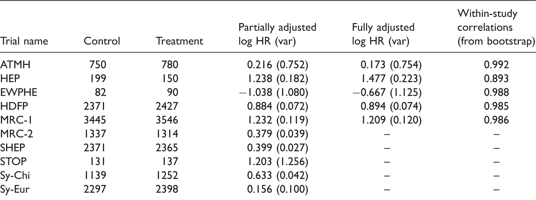
HR: hazard ratio; var: variance.
Upon applying the bivariate meta-analysis, two prior distributions for the between-study variances are considered for comparison. The first is the inappropriate Gamma prior distribution, where 1/τj2∼Gamma(0.1,0.1).
8
The second prior distribution is an empirical prior for future meta-analyses with a binary outcome
10
where
4.2 Results from illustrative example
Key finding (i): The choice of prior distribution for ρB influences the posterior estimates for ρB, and thus borrowing of strength toward βj and joint inferences.
Illustrative example – Summary results from bivariate meta-analysis for various prior distributions for ρB and τj.
CrI: credible interval; SD: standard deviation; U: Uniform; HR: hazard ratio.
Key finding (ii): The choice of prior distribution for τj influences the posterior results for ρB, and thus borrowing of strength toward βj and joint inferences.
Posterior mean and 95% CrI for between-study correlation for various prior distributions in the illustrative example.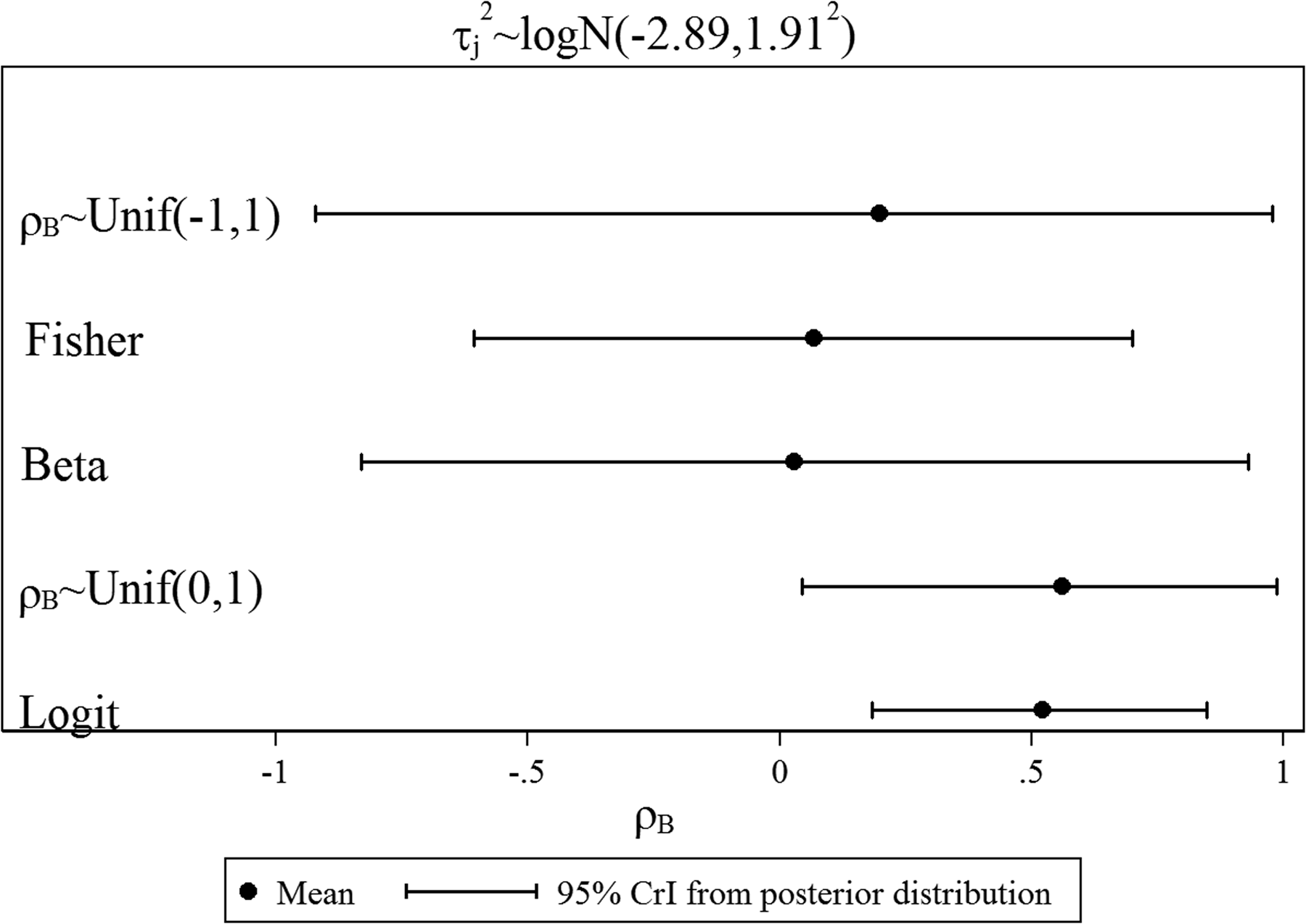
Key finding (iii): The prior distribution for ρB also influences the posterior estimates for τj.
Posterior median and 95% CrI for between-study variances and between-study correlation for the two selected prior distributions for the between-study variances.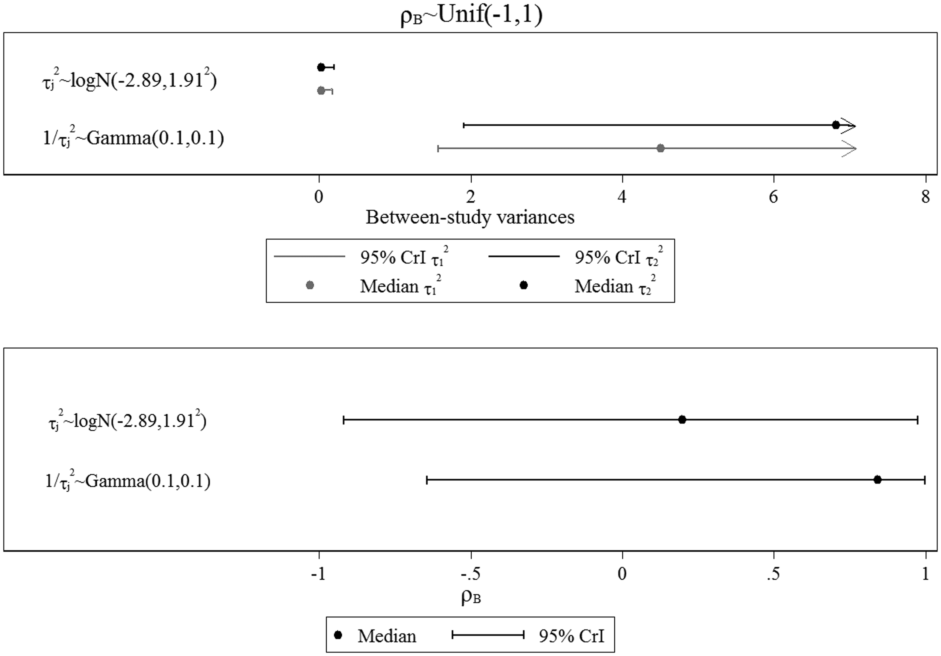
Key finding (iv): The Gamma prior distribution for 1/τj
2
is inappropriate and empirically based prior distributions are preferred for multivariate meta-analysis.
Posterior median and 95% CrI for between-study variance for fully adjusted logHR for various priors for between-study correlation.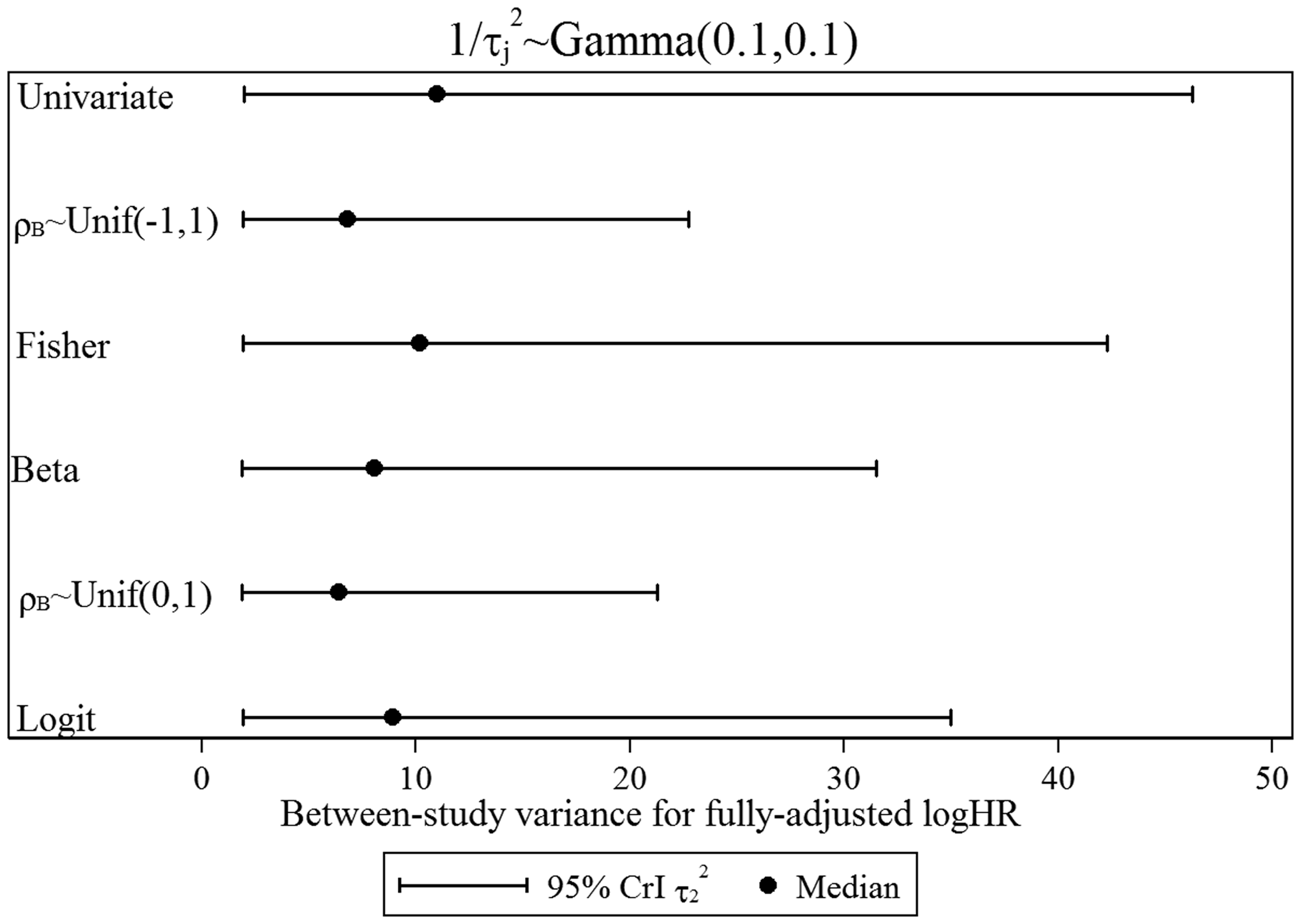
Therefore, empirically based prior distributions for between-study variances are highly preferable in the multivariate meta-analysis field. Similarly, empirically based prior distributions for the between-study correlation are needed where possible, to ensure that the borrowing of strength and joint inferences are appropriate. The commonly chosen Uniform(−1,1) prior distribution may not always be appropriate.
5 Discussion
In a meta-analysis of multiple effects, a multivariate approach can jointly synthesise the endpoints and account for any correlation between the effects that may exist both within and between studies.5,33 This leads to borrowing of strength and thus potentially different and stronger conclusions than separate univariate analyses, and therefore, within a Bayesian bivariate meta-analysis framework, it is crucial for prior distributions to be selected with care. This paper has explored the choice of prior distributions for the between-study variances and correlation in a Bayesian bivariate random-effects meta-analysis within a simulation study and a real example. The key recommendations are summarised in Box 1 and now briefly discussed.
The use of a Wishart prior distribution on the entire between-study variance-covariance matrix is best avoided; it can be highly influential toward posterior meta-analysis results. Rather, a separate prior distribution should be specified for the between-study variances and the correlation. The prior distributions for between-study variances need to be chosen sensibly as they strongly impact on parameter estimates including the between-study correlation, and thus can influence the amount of borrowing of strength and subsequent joint inferences. For this purpose, empirical prior distributions may be most useful, such as those by Rhodes et al.
9
and Turner et al.
10
The use of an inverse Gamma prior distribution is best avoided. The prior distribution for the between-study correlation also needs to be chosen sensibly, as it may have large influence toward the amount of borrowing of strength and joint inferences, especially when the number of studies providing both outcomes is small and the between-study variation is relatively small. A Uniform(−1,1) prior distribution for ρB is not always vague and thus should not be routinely used without due thought. Even when the number of studies is large (say, 50) it can have an important influence when the true correlation is large. Clinical, biological, or methodological rationale might provide external evidence to inform a more realistically vague prior distribution for the between-study correlation. For example, a Uniform(0,1) prior distribution could be specified if only positive values are plausible, such as prognostic effects that are partially and fully adjusted, or treatment effects on two highly correlated outcomes like systolic and diastolic blood pressure. A Uniform(−1,0) prior distribution might be specified if only negative values are plausible, for example for sensitivity and specificity from multiple studies that use different thresholds. Sensitivity analysis for the choice of prior distributions on between-study variances and correlations may be needed, especially when external evidence to inform the prior distributions is not available, borrowing of strength is potentially large (due to missing data), and there is relatively small information from the likelihood to inform their posterior distributions (for example, when the number of studies in the meta-analysis is small, and the between-study variance is small relative to the within-study variances).
5.1 Key findings
In current applications of multivariate meta-analysis, the Uniform(−1,1) distribution is often selected for the between-study correlation without a sensitivity analysis,1,17,18 perhaps assuming it is vague. However, this work illustrates that the choice of prior distribution for ρB is often highly informative of posterior conclusions for all parameters of interest, especially when there are few studies in the meta-analysis, or missing outcome data. Even with large numbers of studies, such as 50, the prior distribution still noticeably influences the posterior distribution for the between-study correlation, which can impact upon the amount of borrowing of strength, joint inferences and subsequently clinically important measures such as the summary treatment effects and probabilistic statements. Therefore, a major recommendation is that the prior distribution for the between-study correlation must be chosen carefully in future multivariate meta-analyses, and the commonly chosen Uniform(−1,1) prior distribution is not always appropriate.
Although appropriate estimation of the between-study correlation is important in complete data settings (especially, when making joint inferences across the multiple outcomes), it is even more critical in missing data settings. The prior distribution is more informative of the posterior distribution for this parameter since there is less data to estimate the between-study correlation, and the correlation itself has more impact on the borrowing of strength, which is usually greater in missing data settings. 5 Therefore, a sensible prior distribution for the between-study correlation is desired. External sources of data, such as similar systematic reviews, could be used to construct plausible prior distributions for this parameter.21,26,29 If related data are unavailable, a clinically relevant range of values for the prior distribution could still be specified. For example, if the meta-analysis pools overall and progression-free survival, it may be clinically plausible that the correlation is restricted to positive values only, and therefore, a Uniform(0,1) prior distribution may be more realistic than a Uniform(−1,1) distribution. Alternatively, if a meta-analysis is used to pool sensitivity and specificity estimates from diagnostic test studies, the correlation could be restricted to negative values, and the Uniform(–1,0) prior distribution may be a sensible choice. If negative (or positive) values are highly unlikely but not implausible, then a distribution might be used that allows all values but with most probability given to positive (or negative) values (see Supplementary Material). If there is no prior information to inform a more realistically vague prior distribution, then the Uniform(−1,1) distribution appears the most sensible choice. However, a sensitivity analysis that considers alternative prior distributions would then be especially important.
The choice of prior distribution for the between-study correlation and the between-study variances are not independent, and therefore, wise choices must be made for all parameters in the bivariate meta-analysis model. Where previous simulation work has illustrated the importance of the prior distribution for the between-study variance in a univariate meta-analysis, 8 the simulation studies in this paper reveal that this is also true for a bivariate meta-analysis. If an inappropriate prior distribution is selected for the between-study variance, this not only has an impact on the posterior estimates of τj themselves but also on the posterior estimate of between-study correlation, the pooled treatment effect estimates, the amount of borrowing of strength, and subsequently joint inferences. Therefore, previously derived empirical prior distributions9–11 should be considered for the between-study variance parameters in a multivariate setting. The use of Gamma or Wishart prior distributions should be avoided; our simulation study shows this may introduce bias in the posterior estimates of the between-study variances and correlation, which then may influence the subsequent meta-analysis results and borrowing of strength. This was previously noted as a potential concern by Achana et al. 41 in a single application of network meta-analysis of multiple treatments and outcomes. However, Wishart prior distributions are still being suggested by some researchers, for example, in a recent tutorial for undertaking Bayesian bivariate meta-analyses. 42
5.2 Limitations
Whilst many different prior distributions were examined, there are, of course, numerous other prior distributions that could be used but were not considered here. Furthermore, the simulation study was specifically for bivariate meta-analysis, but there may be more than two correlated outcomes. In this case, there are several more between-study variance-covariance parameters that require prior distributions. However, the findings are likely to generalise.
Finally, the simulation results (e.g. bias, MSE, coverage) are essentially a frequentist evaluation of a Bayesian analysis, which some may argue may not be appropriate. In particular, Senn 43 previously suggested that it is perhaps philosophically incorrect to conduct a simulation study to assess the performance of Bayesian prior distributions because it is ‘irrelevant to any Bayesian who truly believed what the prior distribution represented’. Although this is an important statement, the rationale for the simulation study here is similar to that of Lambert et al. 44 who justify that, ‘if a statistician desires to have a model with good bias and coverage properties, but needs/wants to use Bayesian methods, then we believe that simulation is a very good way of establishing this’.
5.3 Conclusions
The simulation study and the illustrative example revealed that the choice of prior distribution for the between-study correlation in a Bayesian bivariate random-effects meta-analysis is important and must be chosen with caution, and in conjunction with suitable choices of prior distributions for the between-study variances. Ideally, the empirical prior distributions should be utilised for the between-study variance parameters, and external clinical evidence used to inform a realistically vague prior distribution of the between-study correlation. This is especially important for multivariate meta-analysis involving missing data, where the correlation dictates the amount of borrowing of strength from indirect information, and when joint inferences are desired across the multiple effects of interest. Often, sensitivity analyses to the choice of all prior distributions will be essential.
Box 1 summarises recommendations for future Bayesian multivariate random-effects meta-analyses.
Footnotes
Acknowledgements
We would like to thank Dan Jackson and Ian White for helpful feedback during the initial stages of the project, and also two anonymous reviewers for their constructive feedback on how to improve the paper.
Author contributions
RR and SB conceived the research idea. DB undertook all the simulation analyses under the supervision of RR and feedback from SB. DB drafted the paper and revised following comments from RR and SB.
Declaration of conflicting interests
The author(s) declared no potential conflicts of interest with respect to the research, authorship, and/or publication of this article.
Funding
The author(s) disclosed receipt of the following financial support for the research, authorship, and/or publication of this article: Richard D Riley was supported by funding from a multivariate meta-analysis grant from the MRC Methodology Research Programme (grant reference number: MR/J013595/1). Danielle Burke was partly supported by funding from the MRC Midlands Hub for Trials Methodology Research, at the University of Birmingham (Medical Research Council Grant ID G0800808). Sylwia Bujkiewicz is supported by the Medical Research Council (MRC) Methodology Research Programme (New Investigator Research Grant MR/L009854/1).
Supplement Material
Supplementary material is available for this article online.
References
Supplementary Material
Please find the following supplemental material available below.
For Open Access articles published under a Creative Commons License, all supplemental material carries the same license as the article it is associated with.
For non-Open Access articles published, all supplemental material carries a non-exclusive license, and permission requests for re-use of supplemental material or any part of supplemental material shall be sent directly to the copyright owner as specified in the copyright notice associated with the article.