Sage Journals: Discover world-class research

Abstract

Observational studies are increasingly being used to estimate the effect of treatments, interventions and exposures on outcomes that can occur over time. Historically, the hazard ratio, which is a relative measure of effect, has been reported. However, medical decision making is best informed when both relative and absolute measures of effect are reported. When outcomes are time-to-event in nature, the effect of treatment can also be quantified as the change in mean or median survival time due to treatment and the absolute reduction in the probability of the occurrence of an event within a specified duration of follow-up. We describe how three different propensity score methods, propensity score matching, stratification on the propensity score and inverse probability of treatment weighting using the propensity score, can be used to estimate absolute measures of treatment effect on survival outcomes. These methods are all based on estimating marginal survival functions under treatment and lack of treatment. We then conducted an extensive series of Monte Carlo simulations to compare the relative performance of these methods for estimating the absolute effects of treatment on survival outcomes. We found that stratification on the propensity score resulted in the greatest bias. Caliper matching on the propensity score and a method based on earlier work by Cole and Hernán tended to have the best performance for estimating absolute effects of treatment on survival outcomes. When the prevalence of treatment was less extreme, then inverse probability of treatment weighting-based methods tended to perform better than matching-based methods.

Keywords

propensity score survival analysis inverse probability of treatment weighting Monte Carlo simulations observational study time-to-event outcomes

1 Introduction

Health researchers are increasingly using observational studies to estimate the effects of treatments, interventions and exposures on outcomes. In observational studies, due to the lack of random treatment assignment, treated or exposed subjects frequently differ from untreated or unexposed subjects. It is thus essential that statistical methods are used to remove or minimize the effects of confounding due to differences in the distribution of observed or measured baseline covariates between treatment groups when estimating the effects of treatments or exposures.

Propensity score methods are increasingly being used to reduce or minimize the confounding that occurs frequently in observational studies of the effect of treatment on outcomes.^1,2 The propensity score is the probability of treatment assignment conditional on measured baseline covariates.³ There are four ways of using the propensity score to reduce confounding: matching on the propensity score, stratification on the propensity score, inverse probability of treatment weighting using the propensity score and covariate adjustment using the propensity score.^3–6

When outcomes are binary, the effect of treatment can be reported using relative measures of effect (the odds ratio and the relative risk) and absolute measures of effect (the risk difference or the absolute risk reduction), along with the number needed to treat (NNT) (the reciprocal of the absolute risk reduction). Schechtman argued that both relative and absolute measures should be reported,⁷ whereas Jaeschke et al. suggest that relative measures of effect provide limited information.⁸ Cook and Sackett argue that for clinical decision making the NNT is more meaningful than relative measures of effect.⁹ Finally, Sinclair and Bracken argue that clinically important questions are best addressed using all four measures of effect.¹⁰ In the face of these proposals, some medical journals require that the NNT be reported for any randomized controlled trial with a dichotomous outcome.¹¹ Substantial research has been conducted on examining the performance of different propensity score methods when outcomes are binary.^3,12–15

In biomedical research, time-to-event outcomes occur frequently.¹⁶ When outcomes are time-to-event in nature, both relative and absolute measures of effect can be reported. The hazard ratio provides a relative measure of effect: the relative difference in the treatment-specific hazard rates which mirror the event probabilities in an infinitesimal time interval [t, t + Δ), given the condition that an individual was event-free until time t. Absolute change in mean or median survival time is an absolute measure of effect that can be used with time-to-event outcomes. Similarly, one can estimate the absolute reduction in the probability of the occurrence of an event within a specified duration of follow-up. This latter quantity allows one to estimate the NNT to avoid the occurrence of one outcome within the specified duration of follow-up. Relative effect of treatment on survival outcomes appear to be reported with much greater frequency than absolute measures of effect. However, as stated in the previous paragraph, the consensus of clinical commentators suggests that medical decision making is best informed by the reporting of both relative and absolute measures of effect. Two recent papers have examined the performance of propensity score methods for estimating hazard ratios.^17,18 However, there is a paucity of research examining the performance of different propensity score methods for estimating absolute effects of treatment on survival outcomes.

Accordingly, the objective of this study was to examine the ability of different propensity score methods to estimate absolute effects of treatment on survival outcomes. The article is structured as follows: in Section 2, we describe different propensity score methods and how they can be used to estimate absolute effects of treatment on survival outcomes. In Section 3, we describe the design of an extensive series of Monte Carlo simulations to compare the performance of different propensity score methods for estimating absolute effects of treatment on survival. In Section 4, we present the findings from our Monte Carlo simulations. Finally, in Section 5, we summarize our findings and place them in the context of the existing literature.

2 Propensity score methods and estimating absolute effects on survival outcomes

In this section, we briefly describe the different propensity score methods that were examined for estimating absolute effects of treatment on survival outcomes. We use the following notation throughout this section. Let Z be an indicator variable denoting treatment status (Z = 1 for active treatment of interest vs. Z = 0 for the control treatment), while e denotes the estimated propensity score. In the first three subsections, we describe how survival functions comparing survival between treated and untreated subjects can be estimated that remove the effects of confounding due to observed covariates. These survival functions are marginal survival functions: they describe survival in a population of subjects in which all subjects are treated or in which all subjects are untreated. In the fourth subsection, we describe how absolute effects of treatment on survival can be estimated once these marginal survival functions have been estimated.

2.1 Matching on the propensity score

Matching on the propensity score entails forming matched sets of treated and untreated subjects who have a similar value of the propensity score.¹⁹ We used two different algorithms to form matched pairs of treated and untreated subjects. First, we used greedy nearest neighbour matching without replacement to match treated subjects to the untreated subject whose propensity score was closest to that of the treated subject. Second, we used greedy nearest neighbour caliper matching. We matched subjects on the logit of the propensity score,¹⁹ using calipers of width equal to 0.2 of the standard deviation of the logit of the propensity score, as this caliper width has been found to perform well in a wide variety of settings.²⁰ We refer to these two methods as nearest neighbour matching and caliper matching, respectively. Pair-matching allows one to estimate the average treatment effect on the treated (ATT): the average effect of treatment in those subjects who ultimately received the treatment.

Once a propensity score matched sample has been formed, one can estimate marginal survival functions using the Kaplan–Meier estimator. Separate survival functions can be estimated in treated and untreated subjects in the propensity score matched sample. The survival function estimated in treated subjects represents the marginal survival function in the treated population had all subjects been treated. The survival function estimated in untreated subjects represents the marginal survival function in the treated population had all subjects been untreated.

2.2 Stratification on the propensity score

Stratification (or subclassification) on the propensity score stratifies the entire sample into mutually exclusive subclasses based on the propensity score. A common approach is to define the subclasses using specified quantiles of the propensity score. Using the quintiles of the estimated propensity score to divide the sample into five, approximately equally sized, groups has been shown to eliminate approximately 90% of the bias due to measured confounding variables when estimating a linear treatment effect.^3,4,21 We used stratification on the quintiles of the propensity score in this study given its popularity in the applied literature.

We used stratification on the propensity score to estimate marginal survival curves for each of the two treatment groups as follows: first, in each of the propensity score strata, we estimated Kaplan–Meier survival curves in treated and untreated subjects separately. Let S₀ _j (t) and S₁ _j (t) denote the estimated survival curve in untreated and treated subjects, respectively, in the jth stratum. Then, an estimate of the marginal survival curve in untreated subjects is $S_{0} (t) = \sum_{j = 1}^{K} p_{j} S_{0 j} (t)$ , where K denotes the number of strata, and p_j denotes the stratum-specific weights for pooling the stratum-specific marginal survival curves (such that $\sum_{j = 1}^{K} p_{j} = 1$ ). When estimating the effect of treatment in the overall population (i.e. the average treatment effect or the ATE), the strata would be weighted equally, and each p_j = 1/K (since the same proportion of subjects in the overall sample lie within each stratum). When estimating the ATT, each stratum would be weighted proportionally to the number of treated subjects who lay within that stratum. Essentially, one is pooling stratum-specific survival curves to obtain a population-average survival curve. The marginal survival curve in treated subjects, S₁(t), can be estimated similarly.

2.3 Inverse probability of treatment weighting using the propensity score

The inverse probability of treatment weights (IPTWs) are defined as $\frac{Z}{e} + \frac{1 - Z}{1 - e}$ .²² Estimated treatment effects are not confounded in the sample weighted using the IPTWs, if all confounding baseline covariates are considered. Furthermore, in the weighted sample, the distribution of baseline covariates in each treatment group will be the same as the distribution of baseline covariates in the overall unweighted sample.²³ Using these weights allows one to estimate the ATE. Using weights equal to $Z + \frac{e (1 - Z)}{1 - e}$ allows one to estimate the ATT.²⁴ When using ATT weights, the distribution of baseline covariates in each treatment group in the weighted sample will be the same as the distribution of baseline covariates in treated subjects in the original, unweighted sample. We examined two different methods with which IPTWs can be used to estimate survival functions, and therefore absolute effects on survival outcomes.

2.3.1 Xie and Liu’s adjusted Kaplan–Meier estimator and weighted log-rank test

Xie and Liu proposed an adjusted Kaplan–Meier estimator of the survival function in treated and untreated subjects that allows one to account for confounding by incorporating IPTWs.²⁵ Furthermore, they used method of moment formulas to derive an adjusted log-rank test for use with the weighted sample. Both the adjusted Kaplan–Meier estimate and the adjusted log-rank test reduce to the conventional Kaplan–Meier estimate and the conventional log-rank test in the case that the weights are all equal to one.

2.3.2 Cole and Hernán’s adjusted survival curves with inverse probability weights

Cole and Hernán described a method to estimate adjusted survival curves using inverse probability weights.²³ They proposed that a null Cox proportional hazards regression model be fit separately in treated and untreated subjects (alternatively, a null model is fit that stratifies on treatment status). The model is fit in the sample weighted by the IPTWs. From the fitted regression model, survival curves can be estimated for treated and untreated subjects separately. They note that when the weights are non-parametrically estimated, the described method is equivalent to direct standardization of the survival curves to the overall study population.

2.4 Estimating absolute treatment effects using marginal survival functions

Once marginal survival functions had been estimated for treated and untreated subjects, we estimated the effect of treatment on mean survival as follows: first, the mean survival time in each of the two treatment groups was estimated by calculating the area under the estimated survival curve in the respective treatment groups using trapezoidal integration.²⁶ Second, the effect of treatment on mean survival time was estimated as the difference between mean survival in the treated subjects and mean survival in the untreated subjects. The effect of treatment on changes in median survival time can be estimated similarly. Using each of the two marginal survival curves, one can estimate median survival time under treatment and under lack of treatment. The effect of treatment on median survival time can be estimated using the difference in these two quantities.

We also estimated the effect of treatment on the absolute reduction in the probability of the occurrence of the event within specific durations of follow-up time. Using the two marginal survival curves, we estimated the probability of survival to a specified time t₀. Let S_k(t₀) denote the probability of survival to time t₀ in treatment group k (k = 0 (untreated) or k = 1 (treated)). Then, the absolute reduction in probability of the occurrence of an event prior to time t₀ was estimated as S₀(t₀) − S₁(t₀).

3 Monte Carlo simulations – methods

We used a series of Monte Carlo simulations to examine the performance of different propensity score methods to estimate the absolute effect of treatment on survival or time-to-event outcomes. Our simulations used a design similar to that used in a recent study comparing the performance of different propensity score methods for estimating marginal hazard ratios.¹⁷

3.1 Data-generating process

We simulated data for a setting in which there was 10 baseline covariates ( $X_{1} - X_{10}$ ). These covariates were simulated from independent standard normal distributions. Of these 10 covariates, 7 affected treatment selection (X₁ − X₇), while 7 affected the outcome (X₄ − X₁₀). For the ith subject, the probability of treatment selection was determined from the following logistic model: $logit (p_{i}) = α_{0, treat} + α_{W} x_{1 i} + α_{M} x_{2 i} + α_{S} x_{3 i} + α_{W} x_{4 i} + α_{M} x_{5 i} + α_{S} x_{6 i} + α_{VS} x_{7 i}$ . The intercept of the treatment-selection model (α_0,treat) was selected so that the proportion of subjects in the simulated sample that were treated was fixed at a desired proportion. The regression coefficients α _W , α _M , α _S , α _VS were set to log(1.25), log(1.5), log(1.75) and log(2), respectively. These were intended to denote weak, moderate, strong and very strong treatment-assignment effects. For each subject, treatment status was generated from a Bernoulli distribution with subject-specific parameter p_i: Z_i ∼ Be(p_i).

We then generated an observed time-to-event outcome for each subject using a data-generating process for time-to-event outcomes described by Bender et al.²⁷ For each subject, the linear predictor was defined as ${LP}_{i} = β_{treat} z_{i} + α_{W} x_{4 i} + α_{M} x_{5 i} + α_{S} x_{6 i} + α_{VS} x_{7 i} + α_{W} x_{8 i} + α_{M} x_{9 i} + α_{S} x_{10 i}$ . For each subject, we generated a random number from a standard Uniform distribution: u ∼ U(0,1). A survival or event time was generated for each subject as follows: $\frac{- \log (u)}{(λ e LP i) 1 / η}$ . We set λ and η to be equal to 0.00002 and 2, respectively. The use of this data-generating process results in a conditional treatment effect, with a conditional hazard ratio for treatment of exp(β_treat). We used the values of β_treat used in our prior study that were selected to induce specified marginal hazard ratios. Descriptions of how to use a specific conditional effect to induce a desired marginal effect are described in greater detail elsewhere.^17,28,29

We allowed the following factors to vary in our Monte Carlo simulations: the percentage of subjects that were treated (5%, 10% and 25%) and the true marginal hazard ratio (1, 1.10, 1.25, 1.50, 1.75 and 2). We thus examined 18 scenarios (3 treatment prevalences × 6 marginal hazard ratios). In each scenario, we simulated 1000 datasets, each consisting of 10,000 subjects. In our simulation studies, we did not consider censoring; therefore, the simulated true survival time of an individual corresponds to its actual observation time in the study.

3.2 The true effect of treatment

Using the data-generating process described in Section 3.1, we first randomly generated a treatment status for each subject that was conditional on the subject’s baseline covariates. We then used the second data-generating process to randomly generate a survival time that was conditional on both the actual treatment assigned and on the subject’s baseline covariates. We also generated two potential outcomes for each subject: a survival time conditional on the subject having been untreated and a survival time conditional on the subject having been treated. These two potential outcomes were used to determine the true absolute treatment effects.

A Kaplan–Meier estimate of the survival function for the overall population under no treatment was estimated using the set of all potential outcomes under no treatment. Thus, using the potential outcome under no treatment, we estimated the survival function in the overall population. Similarly, a Kaplan–Meier estimate of the survival function for the overall population under treatment was estimated using the set of all potential outcomes under treatment. Trapezoidal integration was used to determine mean survival in the entire population under no treatment and under treatment. The true ATE of the absolute effect of treatment on mean survival time is the difference between these two quantities. Median survival times under treatment and under lack of treatment were estimated using the respective marginal survival functions. The true ATE of the absolute effect of treatment on median survival time is the difference between these two quantities. Similarly, for a given time t₀, one can determine the probability of the event occurring by time t₀ in the entire population if all subjects were treated and again if all subjects were untreated. The difference between these two survival probabilities is the true ATE of the absolute reduction in the probability of the occurrence of the event by time t₀.

ATT values of these different measures of treatment effect can be obtained by restricting the sample of potential outcomes used for estimating survival curves to those of subjects who ultimately received the treatment (i.e. both potential outcomes were used for only those subjects who received the treatment).

These population-average effects determined using both sets of potential outcomes will serve as the gold standard to which each of the different propensity score-based estimates will be compared.

3.3 Statistical analyses in simulated datasets

Within each simulated dataset we estimated the propensity score using a logistic regression model to regress treatment status on the seven baseline covariates that affected the outcome (X₄ − X₁₀). This approach to variable selection for the propensity score model was selected, as it has been shown to result in better estimation compared to selecting only those variables that affect treatment selection.³⁰ In each of the 1000 simulated datasets for each scenario, we estimated the effect of treatment on mean and median survival time using the methods described in Section 2. Similarly, we computed the true effect of treatment on mean survival (estimated from the sample consisting of both potential outcomes for each subject). We then averaged these two quantities (the estimated effect and the true effect) across the 1000 simulated datasets.

Within a simulated dataset, we estimated the 10th, 25th, 50th, 75th and 90th percentiles of the observed survival time. We then estimated the absolute reduction in the probability of the occurrence of the event of interest at each of these five quantiles of survival time. Using the sample consisting of both potential outcomes, we determined the true absolute reduction in the probability of the occurrence of the event of interest at each of these five quantiles of survival time. We then used each of the propensity score methods to estimate the absolute reduction in the probability of the occurrence of the event at each of the five quantiles of survival time.

3.4 Statistical significance testing

We examined the performance of different statistical tests for assessing the statistical significance of the effect of treatment on survival. To do so, we used the simulated datasets in which the true marginal (and conditional) hazard ratio was 1, indicating that the marginal survival functions would be identical between treated and untreated subjects.

In the propensity score matched sample, we considered four different methods for testing statistical significance: (i) the conventional log-rank test in the propensity score matched sample; (ii) the stratified log-rank test in the propensity score matched sample, in which we stratified on the matched pairs; (iii) a Cox proportional hazards regression model was used to regress survival on treatment status. Model-based standard errors were used to assess the significance of the estimated log-hazard ratio of treatment on the outcome; (iv) an approach similar to the previous one, except that the robust standard errors of Lin and Wei were used.³¹ Approaches (i) and (iii) are asymptotically equivalent. However, we include both approaches for the same of completeness. Approaches (ii) and (iv) were intended to account for the potential homogeneity of outcomes within matched sets. Cummings et al. proposed the use of stratification on matched sets to account for matched cohort designs with time-to-event outcomes.³²

When using stratification on the propensity score, methods for comparing the equality of marginal survival curves are less well developed. We considered two different methods: first, we used a Cox proportional hazards regression model to regress survival time on an indicator variable denoting treatment status. The model stratified on propensity score strata, allowing the baseline hazard function to vary across the five propensity score strata. Second, we used the stratified log-rank test in which we stratified on the five propensity score strata.

When using inverse probability of treatment weighting, we used two methods. First, we used Xie and Liu’s adjusted log-rank test. Second, in accordance with the suggestion of Cole and Hernán, we fit a univariate Cox proportional hazards regression model in which survival was regressed on treatment status in the sample weighted by the IPTWs. The robust variance estimator of Lin and Wei was used to estimate the statistical significance of the treatment effect.^23,31

In each of the simulated datasets with a true null treatment effect (true hazard ratio = 1), we determined whether we rejected the null hypothesis of no treatment effect (P < 0.05). We estimated the empirical type I error rate as the proportion of simulated datasets in which we rejected the null hypothesis of no difference in survival between treatment groups. Due to our use of 1000 simulated datasets, an empirical type I error rate <0.0365 or >0.0635 would be statistically significantly different from the advertised rate of 0.05 using a standard normal-theory test.

4 Monte Carlo simulations – results

We describe the results of the Monte Carlo simulations in four subsections: effect of treatment on mean survival time, effect of treatment on median survival time, effect of treatment on the absolute reduction in the probability of the occurrence of event within a specified duration of follow-up and empirical type I error rates. In a fifth subsection, we present some miscellaneous results describing the weights used and the quality of matching.

4.1 Estimation of absolute changes in mean survival time

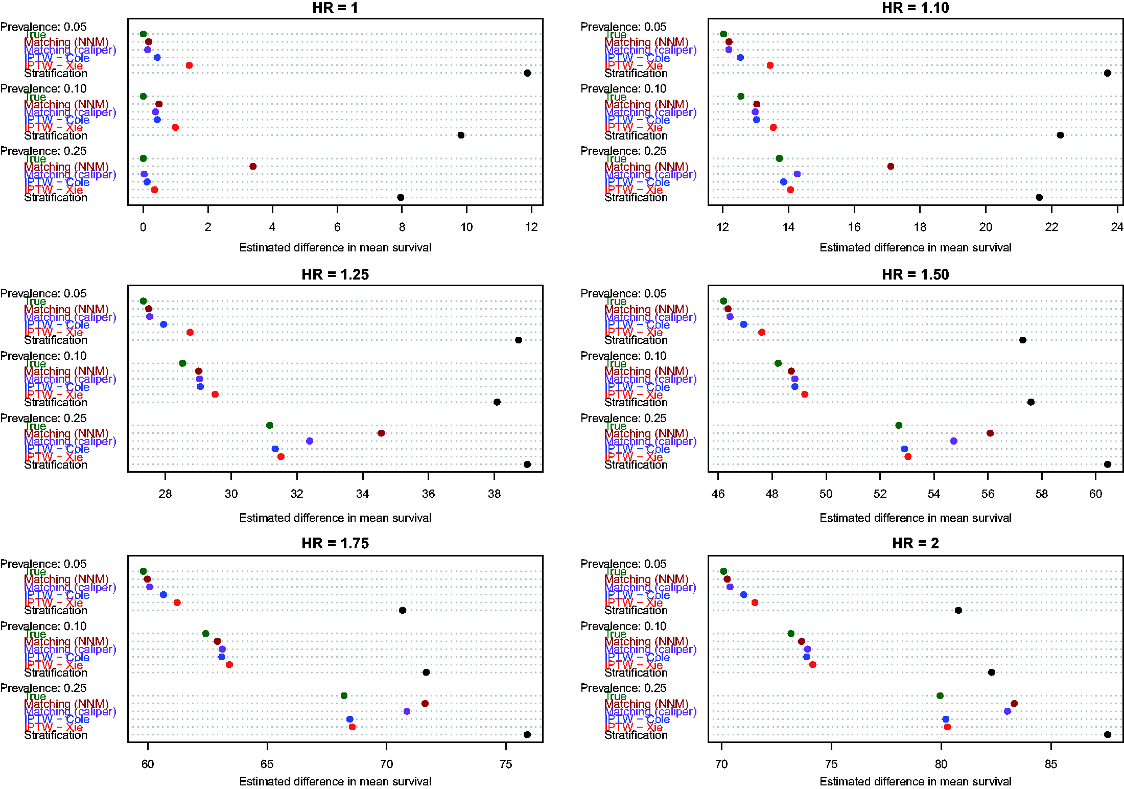
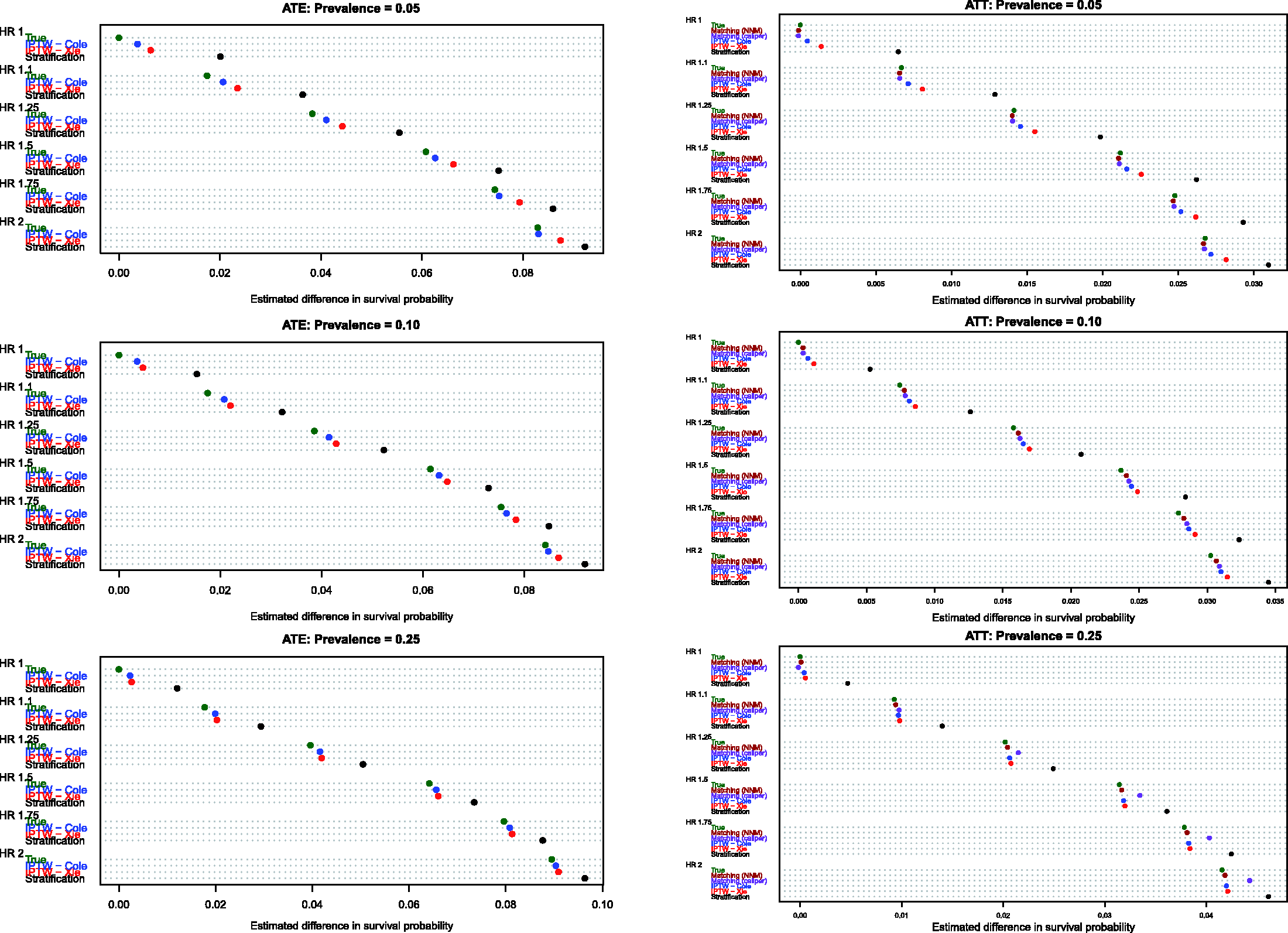
Estimates of the absolute effect of treatment on mean survival time are reported in Figure 1 (effects in the overall population – ATE) and Figure 2 (effects in treated subjects – ATT). Each figure consists of six panels, one for each of the true marginal hazard ratios. In each panel, we use dot charts to represent the true effect of treatment and the estimates of treatment effect obtained using the different propensity score methods. When estimating the effect of treatment in the overall population, estimates using three methods (stratification, Xie and Liu and Cole and Hernán) are compared with the true underlying effect of treatment (computed using both sets of potential outcomes). When estimating the effect of treatment in the treated subjects, two additional methods are added (nearest neighbour matching and caliper matching).

Figure 1.

Estimates of changes in mean survival (ATE).

Figure 2.

Estimates of changes in mean survival (ATT).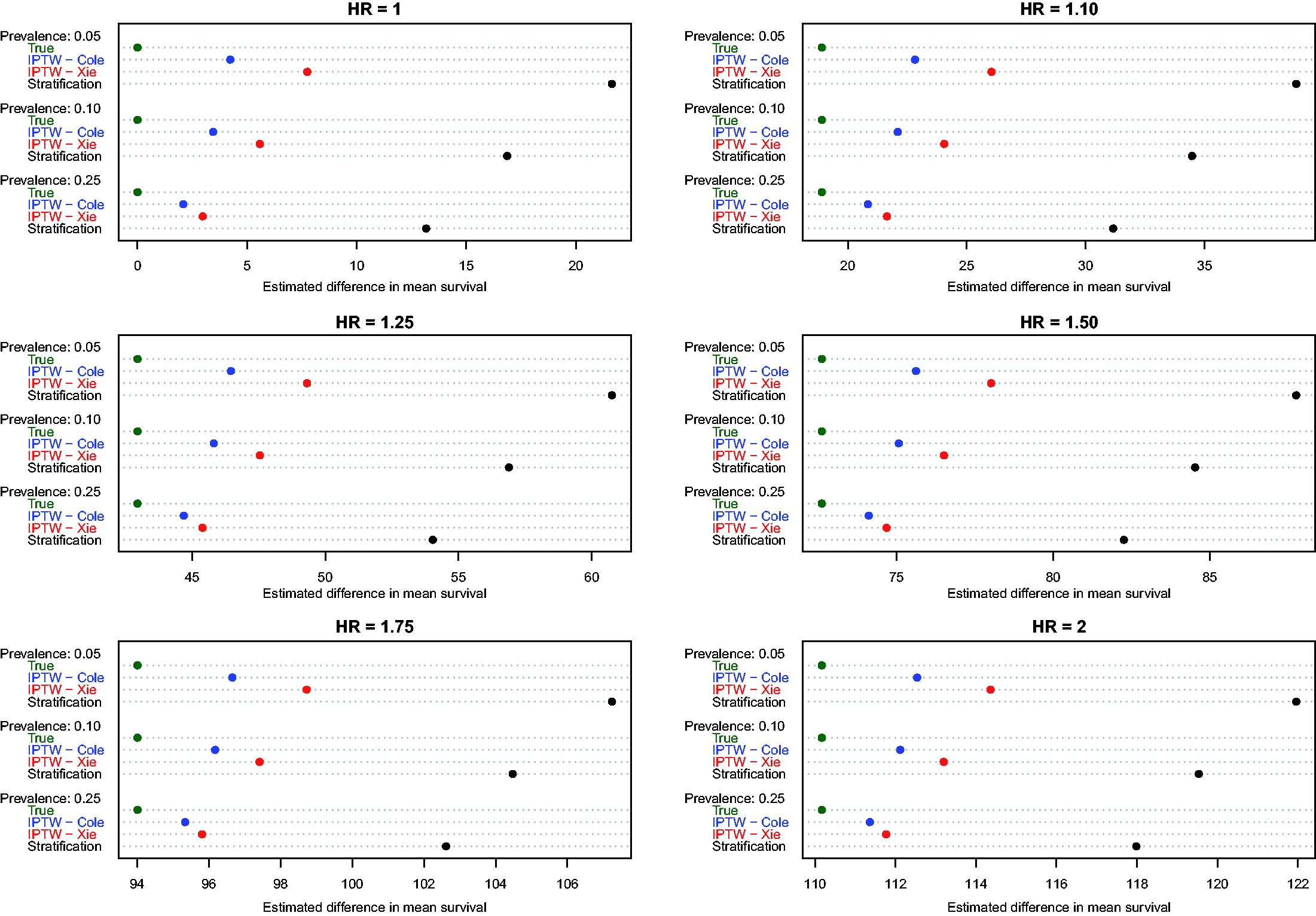

In Figure 1 (effect in entire population), several trends are apparent. First, IPTW using Cole and Hernán’s approach resulted in estimates that were closest to the true absolute change in mean survival due to treatment. The bias due to Xie and Liu’s adjusted Kaplan–Meier estimate was modestly larger than that of Cole and Hernán’s approach. However, for a given marginal hazard ratio, the differences between the two IPTW approaches diminished as the prevalence of treatment increased. Second, stratification resulted in substantially greater bias than the two IPTW methods across all 18 scenarios. Third, the magnitude of the bias diminished slightly when the true underlying marginal hazard ratio was larger. Third, for a given value of the true underlying marginal hazard ratio, the bias for each method decreased as the prevalence of treatment increased.

In examining Figure 2 (effect of treatment in those subjects who were ultimately treated), several observations merit comment. First, as above, stratification resulted in greater bias than all of the other methods across all 18 scenarios. Second, comparing the two IPTW approaches, Cole and Hernán’s method resulted in less biased estimation compared with Xie and Liu’s adjusted Kaplan–Meier estimate across all 18 scenarios. As above, for a given marginal hazard ratio, the differences between these two approaches diminished as the prevalence of treatment increased. Third, nearest neighbour matching and caliper matching had similar performance to one another when the prevalence of treatment was either 5% or 10%. However, when 25% of subjects were treated, bias due to nearest neighbour matching was greater than that due to caliper matching. Furthermore, when 25% of subjects were treated, the differences between these two matching algorithms tended to diminish as the true underlying marginal hazard ratio increased. Fourth, when the prevalence of treatment was low (5% or 10%), then caliper matching tended to result in decreased bias compared with the two IPTW approaches. However, when the prevalence of treatment was 25% and there was a true non-null treatment effect, then caliper matching resulted in greater bias compared with the two IPTW approaches.

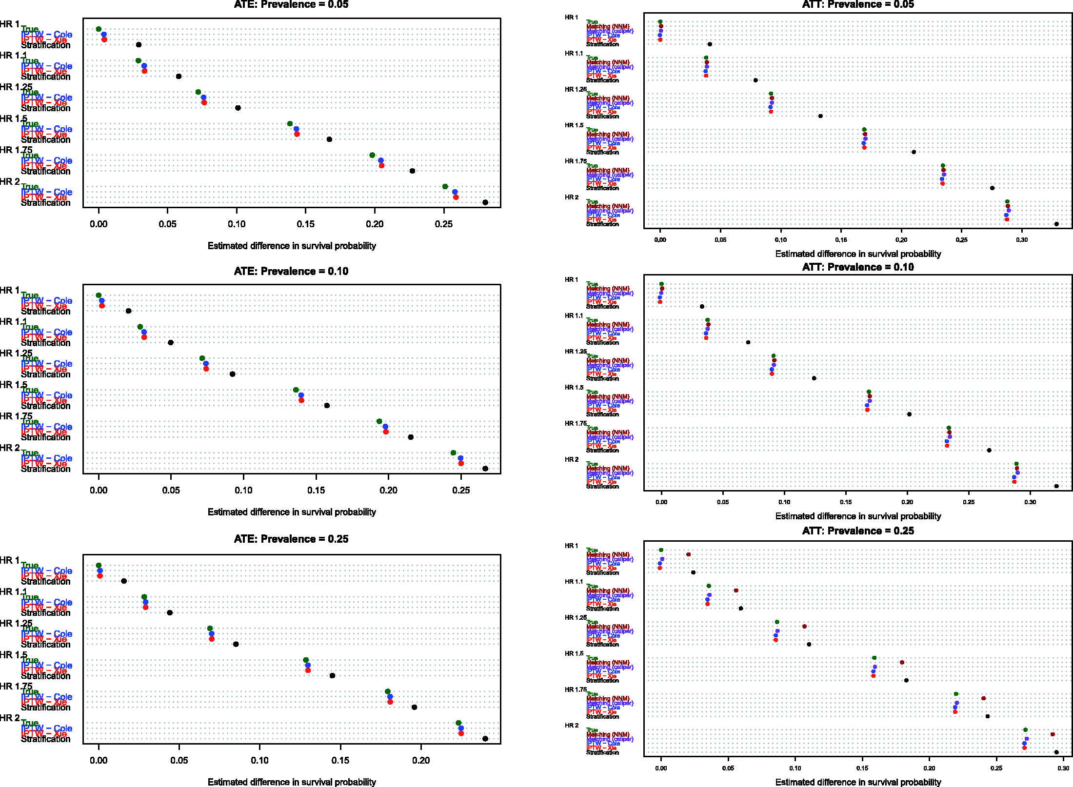
4.2 Estimation of absolute changes in median survival time

Estimates of the absolute effect of treatment on median survival time are reported in Figure 3 (effects in the overall population – ATE) and Figure 4 (effects in treated subjects – ATT). As would be expected when estimating changes in distributions that are positively skewed, changes in median survival tended to be less than the changes in mean survival discussed above. As above, both of the IPTW methods performed better than stratification on the propensity score when estimating changes in median survival time in the entire population. However, compared with estimating changes in mean survival time, differences between the two IPTW approaches were attenuated. In fact, differences between these two approaches tended to be minimal when estimating effects of treatment on median survival time.

Figure 3.

Estimates of changes in median survival (ATE).

Figure 4.

Estimates of changes in median survival (ATT).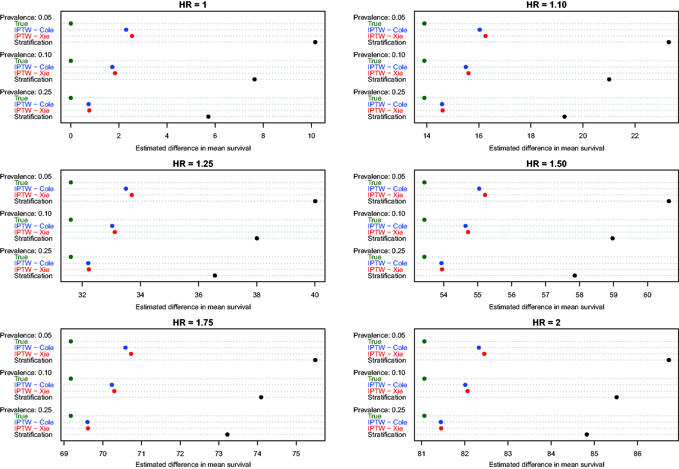

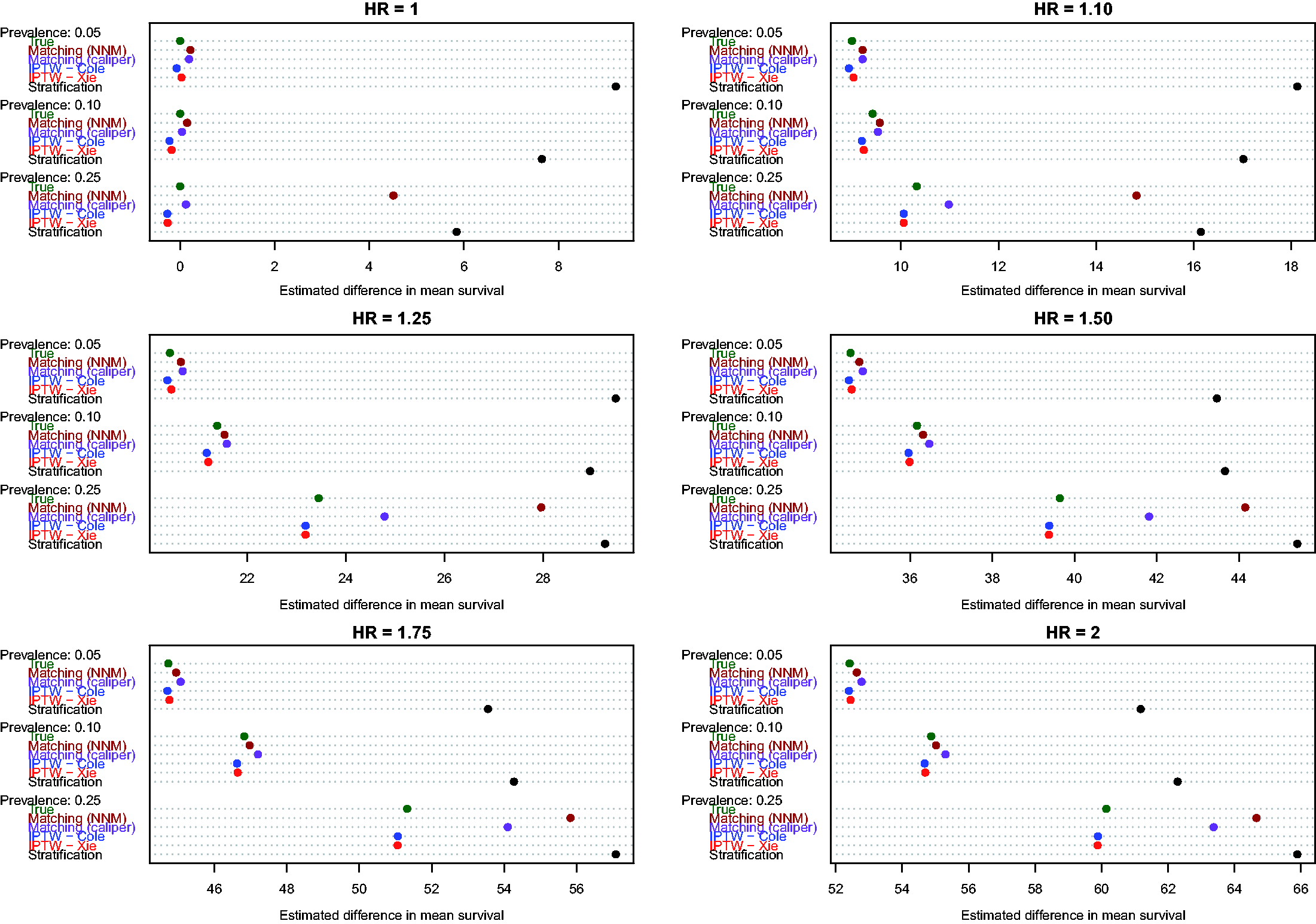
Similarly, when estimating changes in median survival time in the treated population, differences between the two IPTW approaches were minimized. Furthermore, the two IPTW tended to have superior performance compared to the two matching approaches. The differences between the matching approaches and the two IPTW methods tended to be the greatest when 25% of subjects were treated.

4.3 Estimation of the absolute reduction in the probability of the occurrence of the event

Estimates of the absolute effect of treatment on the probability of the occurrence of an event within a given duration of follow-up are reported in Figure 5 (10th percentile of survival times), Figure 6 (25th percentile of survival times), Figure 7 (50th percentile of survival times), Figure 8 (75th percentile of survival times) and Figure 9 (90th percentile of survival times). Each figure has six panels. In each figure, the three panels on the left denote treatment effects in the overall population, whereas the three panels on the right denote treatment effects in the treated population. As noted in Section 4.1, three methods were compared for estimating effects in the overall population, whereas five methods were compared for estimating effects in the treated population.

Figure 5.

Bias in estimating S(10th percentile of t).

Figure 6.

Bias in estimating S(25th percentile of t).

Figure 7.

Bias in estimating S(50th percentile of t).

Figure 8.

Bias in estimating S(75th percentile of t).

Figure 9.

Bias in estimating S(90th percentile of t).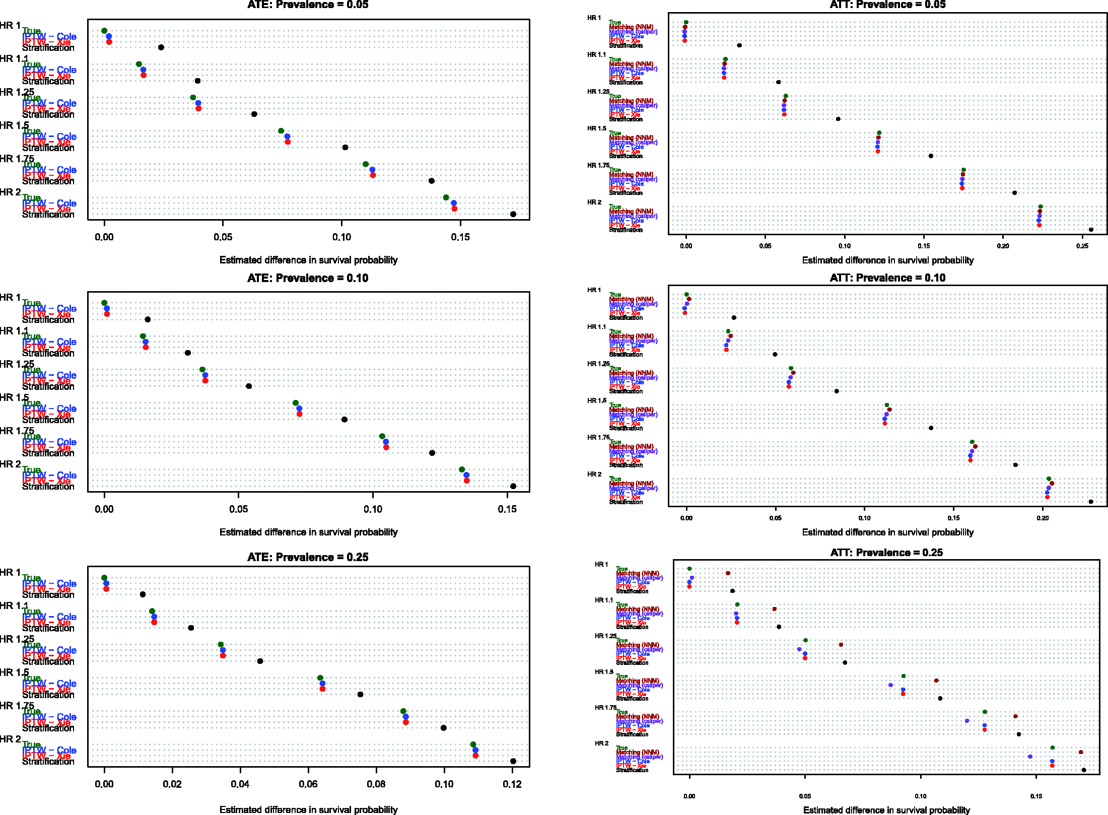

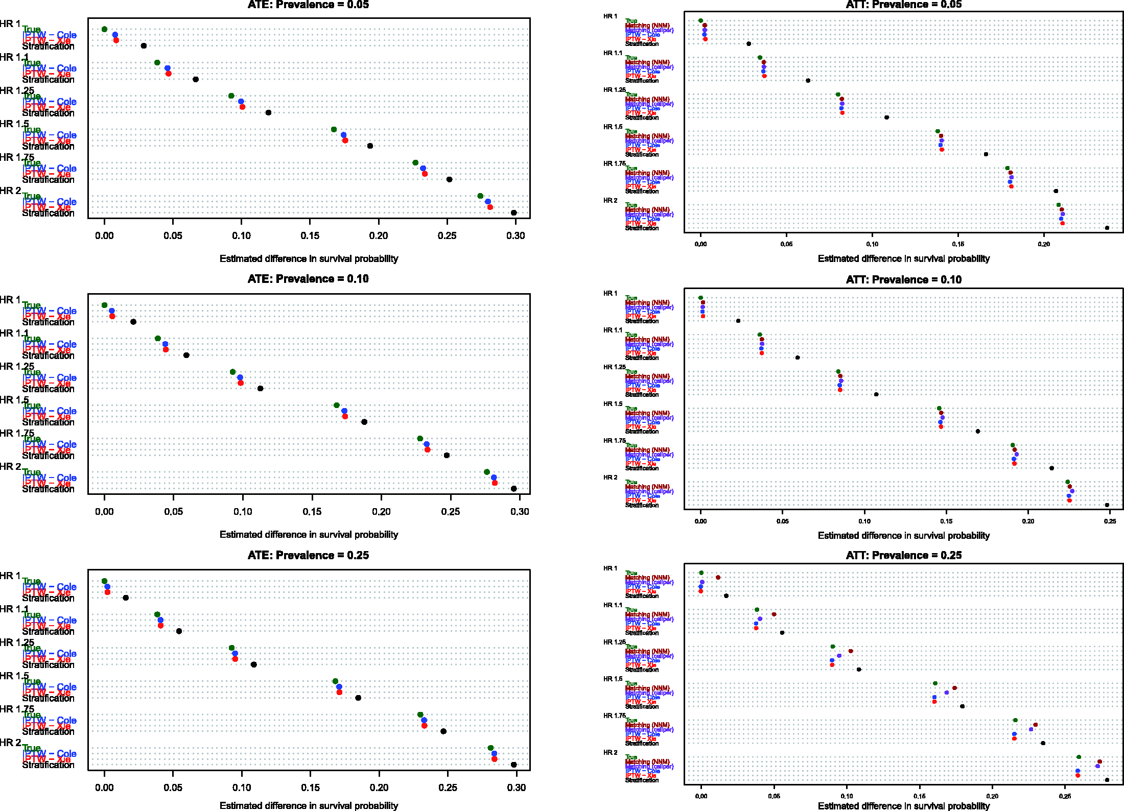
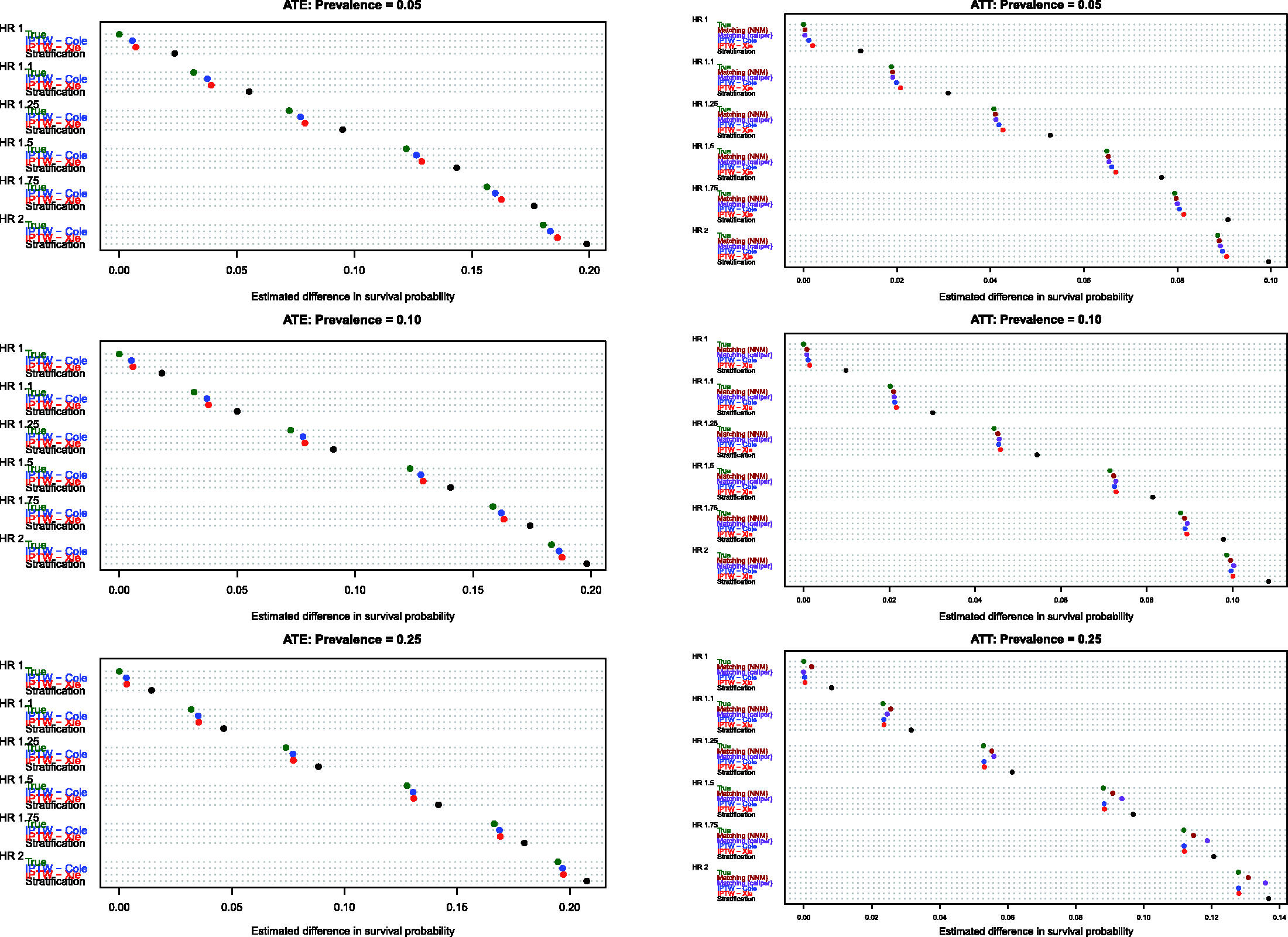
When comparing the performance of the three methods for estimating effects in the entire population, several observations warrant highlighting (see panels in the left column of Figures 5 –9). First, stratification resulted in estimates with greater bias compared with the two IPTW-based methods. Second, for the first four quantiles of survival time (10th, 25th, 50th and 75th percentiles of survival time), the two IPTW approaches resulted in essentially identical estimates of the change in the probability of the occurrence of an event within the given duration of follow-up time. However, when examining estimation at the 90th percentile of survival time, Cole and Hernán’s approach resulted in estimates with slightly less bias than did Xie and Liu’s approach when 5% or 10% of subjects were treated. Third, the bias in the two IPTW approaches was negligible at the four lower quantiles of survival time and was modest at the 90th percentile of survival time.

When comparing the performance of the five methods for estimating effects in the population of treated subjects, several observations warrant highlighting (panels in the right column of Figures 5 –9). First, as above, stratification resulted in the greatest bias across all five methods in all 18 scenarios and across all five quantiles of survival time. Second, for the first three quantiles of survival time (10th, 25th and 50th) and when treatment prevalence was low (5% and 10%), then the two matching methods and the two IPTW methods resulted in essentially unbiased estimates of the absolute change in the probability of the occurrence of an event. Third, for the first three quantiles of survival time and when the prevalence of treatment was 25%, then nearest neighbour matching tended to result in greater bias compared with caliper matching and the two IPTW approaches. Fourth, for the 90th percentile of survival time, the two matching methods tended to have negligibly better performance than the two IPTW methods when the prevalence of treatment was 5% or 10%. However, when the prevalence of treatment was 25%, caliper matching had slightly worse performance than the IPTW methods.

4.4 Empirical type I error rates

Empirical estimates of the type I error rates are reported in Table 1. When comparing survival between treated and untreated subjects in the overall population, stratification on the quintiles of the propensity score had an empirical type I error rate that was substantially higher than the advertised level of 0.05 (range: 0.439–0.629). Similarly, the adjusted log-rank test of Xie and Liu resulted in an inflated empirical type I error rate (range: 0.350–0.722). The approach of Cole and Hernán resulted in empirical type I error rates that were closer to the advertised level (range: 0.051–0.072).

Table 1.

Empirical type I error rates of different propensity score methods for comparing survival functions between treatment groups.

Statistical method	Prevalence of treatment
Statistical method	0.05	0.10	0.25
Effect in overall population of all subjects
Stratification (Cox regression stratifying on PS strata)	0.439	0.571	0.629
Stratification (stratified log-rank test)	0.439	0.572	0.629
IPTW (Cole and Hernán)	0.070	0.072	0.051
IPTW (Xie and Liu)	0.722	0.604	0.350
Effect in population of treated subjects
Caliper matching (naïve Cox regression)	0.013	0.006	0.010
Caliper matching (Cox regression with robust standard errors)	0.034	0.030	0.029
Caliper matching (log-rank test)	0.013	0.006	0.010
Caliper matching (stratified log-rank test)	0.035	0.033	0.039
Nearest neighbour matching (naïve Cox regression)	0.012	0.008	0.073
Nearest neighbour matching (Cox regression with robust standard errors)	0.033	0.030	0.144
Nearest neighbour matching (log-rank test)	0.012	0.008	0.073
Nearest neighbour matching (stratified log-rank test)	0.033	0.033	0.283
IPTW (Cole and Hernán)	0.009	0.006	0.006
IPTW (Xie and Liu)	0.000	0.000	0.000

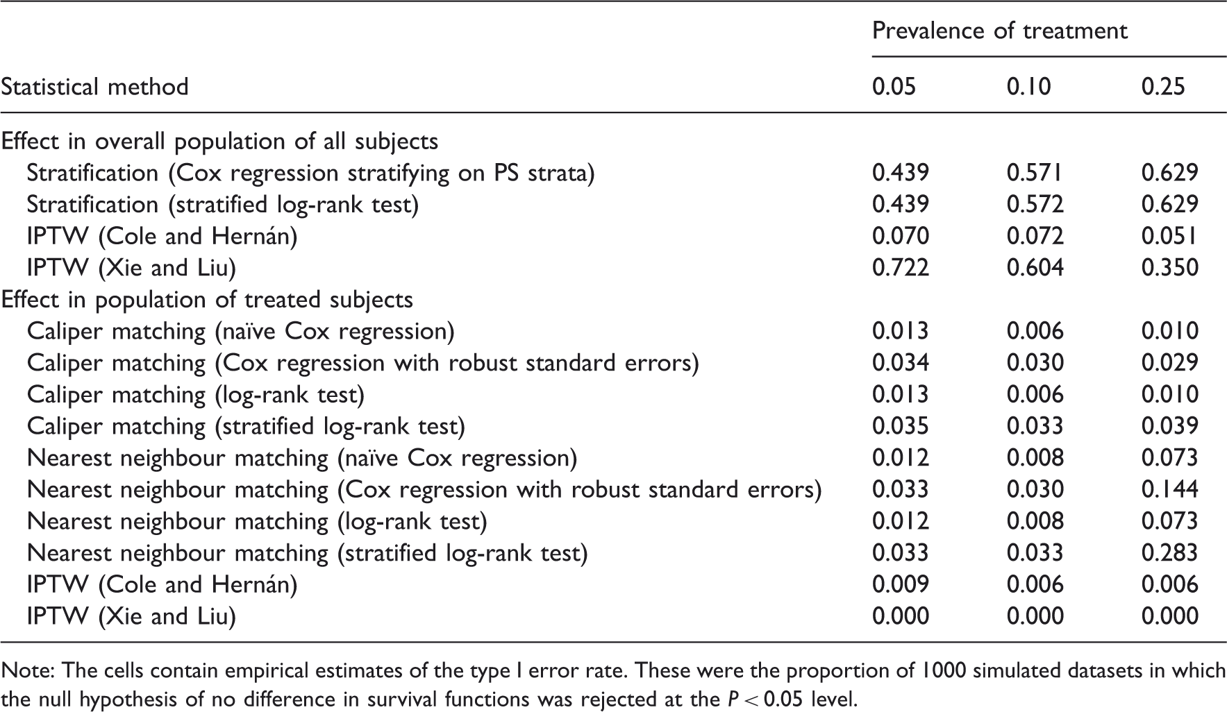
Note: The cells contain empirical estimates of the type I error rate. These were the proportion of 1000 simulated datasets in which the null hypothesis of no difference in survival functions was rejected at the P < 0.05 level.

When comparing marginal survival curves in the population of treated subjects, both the IPTW approaches resulted in artificially low type I error rates (empirical type I error rates <0.01). When using caliper matching, the use of the stratified log-rank test resulted in empirical type I error rates closest to the advertised level (range: 0.033–0.039). The use of the conventional log-rank test resulted in artificially low empirical type I error rates (range: 0.006–0.013). When using nearest neighbour matching, the stratified log-rank test resulted in an inflated type I error rate when the prevalence of treatment was 25% (empirical type I error rate = 0.283).

4.5 Miscellaneous results

Since IPTW analyses can be sensitive to very large weights (occurring when treated subjects have a very low propensity score or untreated subjects have a very high propensity score), we conducted a series of post hoc analyses to examine the distribution of the IPT weights in the simulated datasets. Since the effect of treatment on the hazard of the outcome has no effect on the IPT weights, only the previously described model for the treatment selection process was considered in the subsequent analyses (i.e. the results should be independent of the treatment hazard ratio was used). In the first simulated dataset for each treatment prevalence, we examined the distribution of ATE and ATT weights. We report the following five quantiles for the distribution of the weights for each treatment prevalence and each set of weights: 2.5th, 25th, 50th, 75th and 97.5th (note that we report the distribution of the actual ATT weights. One can invert the summary statistics to examine the distribution on a scale similar to those of the ATE weights; i.e. so that the weights tend to be greater than one). When the prevalence of treatment was 5%, the five-number summary for the ATE weights was 1.01, 1.02, 1.04, 1.08 and 13.06, whereas the five-number summary for the ATT weights was 0.01, 0.02, 0.04, 0.08 and 1. When the prevalence of treatment was 10%, the five-number summary for the ATE weights was 1.01, 1.04, 1.07, 1.16 and 11.80. The corresponding five-number summary for the ATT weights was 0.01, 0.04, 0.07, 0.16 and 1. When the prevalence of treatment was 25%, the five-number summary for the ATE weights was 1.05, 1.17, 1.34, 1.95 and 7.02. The corresponding five-number summary for the ATT weights was 0.05, 0.17, 0.34, 1 and 1.11. One notes that as the prevalence of treatment moves away from 0.5, the upper tail of the distribution of the ATE weights becomes larger (i.e. there is a larger proportion of more larger weights). For the chosen data generation procedure, the amount of large IPT weights is a function of the prevalence. This is due to the fact that the weights are a function of the inverse logit of the linear predictor, and the linear predictors only differed in the intercept among the considered simulation settings. Naturally, there will be a higher proportion of large weights the further away the prevalence gets from 0.5. Therefore, the observed decrease in relative performance of the IPTW approaches with larger amount of unstable weights (lower prevalence) is to be expected.

The mean percentage of treated subjects matched to an untreated subject when using caliper matching was 99.7%, 99.4% and 94.0% when the prevalence of treatment was 5%, 10% and 25%, respectively. Thus, caliper matching only resulted in the exclusion of a small proportion of treated subjects from the matched sample. Therefore, it is likely that minimal bias was introduced due to incomplete matching.¹⁹ The high proportion of treated subjects that were successfully matched to an untreated subject indicates that there was good overlap in the distribution of the propensity score between treatment groups.

5 Discussion

We used an extensive series of Monte Carlo simulations to examine the ability of different propensity score methods to estimate the absolute effects of treatment on survival or time-to-event outcomes. We considered estimating both the absolute effect of treatment on mean and median survival time and the absolute reduction in the probability of the occurrence of the event within a specified duration of follow-up time. We briefly summarize our findings and place them in the context of the existing literature.

Of the different propensity score methods examined, stratification on the propensity score resulted in the greatest bias when estimating the different absolute measures of treatment effect. Coupled with the observation that empirical type I error rate of the stratified analysis was substantially higher than the advertised rate, we would suggest that this method not be used for estimating the absolute effect of treatment on survival outcomes. In prior research, it was shown that stratification on the propensity score resulted in biased estimation of both conditional and marginal hazard ratios.^12,17 These findings complement prior research by Lunceford and Davidian, in which it was shown that stratification on the propensity score can result in biased estimation of linear treatment effects.²² The findings of this study, taken with those of these prior studies, suggest that the use of stratification on the propensity score should be discouraged with survival outcomes.

We examined two different IPTW approaches for estimating absolute effects of treatment on survival outcomes. The first was an adjusted Kaplan–Meier estimate proposed by Xie and Liu, whereas the second was based on the Cox model and was proposed by Cole and Hernán. When estimating the effect of treatment on the absolute change in mean survival time, the latter approach resulted in estimates with modestly less bias than the former method. When estimating the effect on changes in median survival time, the two approaches had comparable performance. When estimating the absolute reduction in the probability of the occurrence of event within a given duration of follow-up (either in the entire population or in the population of treated subjects), both methods had essentially identical performance for the four lower quantiles of survival time (10th, 25th, 50th and 75th percentiles of survival time). When estimating effects at the 90th percentile of survival time, the approach of Xie and Liu resulted in modestly greater bias, especially when the prevalence of treatment was low. We hypothesize that the differences in estimating differences in probabilities at the upper tail of the distribution of event times explains differences in estimating changes in mean survival between these two IPTW approaches. However, it is unclear why these differences in bias exist when estimating survival probabilities at the upper tail of the distribution. When estimating effects in the overall population, the method of Cole and Hernán had an empirical type I error rate that was close to the advertised rate, whereas the empirical type I error rate for the adjusted log-rank test was substantially inflated.

We examined two different matching algorithms: nearest neighbour matching on the propensity score and nearest neighbour matching on the logit of the propensity score within specified calipers. When estimating changes in mean survival time, both approaches resulted in approximately equal bias when the prevalence of treatment was 5% or 10%. However, when the prevalence of treatment was 25%, the use of nearest neighbour matching resulted in substantially greater bias compared with caliper matching (similar biases were seen when estimating the reduction in the probability of the occurrence of an event when the prevalence of exposure was 25%). We suspect that this was due to the inclusion of an increasing number of poor quality matches – matches that would have been excluded when using caliper matching that places a restriction on the quality of the matches. As the proportion of subjects who are treated increases, there are fewer untreated subjects to serve as potential controls. Coupled with the aberrant empirical type I error rates associated with nearest neighbour matching (particularly when the prevalence of exposure was 25%), we suggest that the use of caliper matching be preferred over the use of nearest neighbour matching when estimating absolute effects of treatments on survival outcomes.

When comparing differences in marginal survival functions between treatment groups in the population of subjects who were ultimately treated, the use of the stratified log-rank test in the sample formed by caliper matching resulted in empirical type I error rates that were closest to the advertised rate. Importantly, the use of the conventional log-rank test in the sample constructed using caliper matching resulted in artificially low empirical type I error rates. This reinforces a finding of several prior studies that analyses conducted in the propensity score matched sample should account for the matched nature of the sample.^17,18,33,34 The performance of the two IPTW-based methods with the ATT weights suggests that the performance of these two methods needs to be examined in greater detail when non-ATE weights are used. It was surprising that the choice of weight had such a strong effect on the empirical type I error rate.

The very high empirical type I error rate of the adjusted log-rank test was surprising, given that it was shown to have an acceptable type I error rate in the study in which it was proposed.²⁵ However, in the original paper this was shown using Monte Carlo simulations in a setting in which there was a single binary confounding variable. In a set of secondary analyses, we replicated the data-generating process used in the original paper by Xie and Liu and observed an empirical type I error rate similar to that reported in their paper. We speculate that the findings in this study are attributable to using a more complex and realistic data-generating process in which there were 10 continuous variables which had different effects on the occurrence of the outcome and on treatment selection. This discrepancy suggests that further attention needs to be paid to the variance estimator for the adjusted log-rank test.

When the study objective is to estimate the marginal effect of treatment in the overall population (e.g. the average treatment effect or ATE), we suggest that the IPTW method of Cole and Hernán be used. In some of the 18 scenarios that we examined it had slightly better performance than the approach suggested by Xie and Liu. Furthermore, both IPTW methods performed better than stratification, the only other approach that permits estimation of the ATE.

When the study objective is to estimate the marginal effect of treatment in the population of those who were ultimately treated (e.g. the average treatment effect in the treated or the ATT), then our suggestions are less straightforward and are dependent on the prevalence of treatment and on the estimand of interest. When estimating the effect of treatment on change in median survival time, both IPTW methods resulted in superior performance compared to matching (with the differences between matching and weighting increasing as the prevalence of treatment increased). However, when estimating the effect of treatment on change in mean survival time, we would suggest that caliper matching be used when the prevalence of treatment is low (5% or 10%), while the Cole and Hernán method be used when the prevalence of treatment is higher. When estimating the effect of treatment on the absolute reduction in the probability of the occurrence of an event, then any approach is acceptable if the quantile of survival time is not extreme and the prevalence of treatment is low (5% or 10%). For extreme quantiles of survival time (90th percentile of survival time), then we would recommend the use of caliper matching when the prevalence of treatment is low (5% or 10%). However, when the prevalence of treatment is high (25%), then we would recommend that IPTW methods be used.

There were several limitations to this study that deserve mention. First, when simulating time-to-event outcomes, we did not induce censoring. In subsequent research, the effect of different degrees of censoring on the performance of different methods merits further investigation. This was not investigated in this study for two reasons. First, the simulations were already extensive, with 18 different scenarios. To have introduced a third factor, the degree of censoring, would have substantially increased the amount of results that would need to be communicated. Second, methods for estimating mean survival in the presence of censoring do not always perform well, and a thorough comparison of different methods has not, to our knowledge, been conducted. A second limitation is the reliance of a single set of distributions for the baseline covariates. In subsequent research, it would be informative to examine the robustness of our findings to different distributions of the baseline covariates. However, as with the first limitation, we were unable to examine this in this study due to space and time constraints. A third limitation is that we limited our examination of matching algorithms to two (nearest neighbour matching and nearest neighbour caliper matching). We did not consider alternative algorithms such as optimal matching.³⁵ However, in prior research, it was demonstrated that optimal matching did not induce better balance on measured baseline covariates than competing methods³⁶ and did not result in improved estimation compared to competing methods.³⁷ Thus, we do not expect that optimal matching would have different performance from that of nearest neighbour matching in the context of estimating the effects of treatment on survival outcomes.

Reporting both relative and absolute measures of effect in studies with survival or time-to-event outcomes is essential for making decisions about the benefits, safety and efficacy of treatments and interventions. Many observational studies with survival outcomes have focussed on estimation of hazard ratios. The use of propensity score methods allows for estimation of both relative and absolute measures of effect. In addition to reporting hazard ratios, we recommend that authors report the effect of treatment on mean or median survival time and/or on the absolute reduction in the probability of the occurrence of an event within a specified duration of follow-up. The use of caliper matching on the propensity score and methods based on inverse probability of treatment weighting permit accurate estimation of these quantities.

Footnotes

Acknowledgements

This study was supported by the Institute for Clinical Evaluative Sciences (ICES), which is funded by an annual grant from the Ontario Ministry of Health and Long-Term Care (MOHLTC). The opinions, results and conclusions reported in this paper are those of the authors and are independent from the funding sources. No endorsement by ICES or the Ontario MOHLTC is intended or should be inferred. This research was supported by operating grant from the Canadian Institutes of Health Research (CIHR) (MOP 86508). Dr Austin is supported in part by a Career Investigator award from the Heart and Stroke Foundation. Dr Schuster is supported by a post-doctoral award from the Canadian Network for Observational Drug Effect Studies (CNODES). CNODES is funded by a grant from Health Canada, the Drug Safety and Effectiveness Network (DSEN) and the Canadian Institutes for Health Research (CIHR). The authors are grateful to Jun Xie and Chaofeng Liu for providing R software code for estimating the adjusted Kaplan–Meier estimator and the adjusted log-rank test.

Declaration of conflicting interests

The author(s) declared no potential conflicts of interest with respect to the research, authorship, and/or publication of this article.

Funding

The author(s) received no financial support for the research, authorship, and/or publication of this article.

References

Weitzen

Lapane

Toledano

. Principles for modeling propensity scores in medical research: a systematic literature review. Pharmacoepidemiol Drug Saf 2004; 13: 841–853.

Austin

. A critical appraisal of propensity-score matching in the medical literature between 1996 and 2003. Stat Med 2008; 27: 2037–2049.

Rosenbaum

Rubin

. The central role of the propensity score in observational studies for causal effects. Biometrika 1983; 70: 41–55.

Rosenbaum

Rubin

. Reducing bias in observational studies using subclassification on the propensity score. J Am Stat Assoc 1984; 79: 516–524.

Rosenbaum

. Model-based direct adjustment. J Am Stat Assoc 1987; 82: 387–394.

Austin

. An introduction to propensity-score methods for reducing the effects of confounding in observational studies. Multivariate Behav Res 2011; 46: 399–424.

Schechtman

. Odds ratio, relative risk, absolute risk reduction, and the number needed to treat – which of these should we use? Value Health 2002; 5: 431–436.

Jaeschke

Guyatt

Shannon

. Basic statistics for clinicians: 3. Assessing the effects of treatment: measures of association. Can Med Assoc J 1995; 152: 351–357.

Cook

Sackett

. The number needed to treat: a clinically useful measure of treatment effect. Br Med J 1995; 310: 452–454.

10.

Sinclair

Bracken

. Clinically useful measures of effect in binary analyses of randomized trials. J Clin Epidemiol 1994; 47: 881–889.

11.

http://www.bmj.com/about-bmj/resources-authors/article-types/research (accessed 7 January 2014).

12.

Austin

Grootendorst

Normand

. Conditioning on the propensity score can result in biased estimation of common measures of treatment effect: a Monte Carlo study. Stat Med 2007; 26: 754–768.

13.

Austin

. The performance of different propensity score methods for estimating marginal odds ratios. Stat Med 2007; 26: 3078–3094.

14.

Austin

. The performance of different propensity-score methods for estimating relative risks. J Clin Epidemiol 2008; 61: 537–545.

15.

Austin

. The performance of different propensity-score methods for estimating differences in proportions (risk differences or absolute risk reductions) in observational studies. Stat Med 2010; 29: 2137–2148.

16.

Austin

Manca

Zwarenstein

. A substantial and confusing variation exists in handling of baseline covariates in randomized controlled trials: a review of trials published in leading medical journals. J Clin Epidemiol 2010; 63: 142–153.

17.

Austin

. The performance of different propensity score methods for estimating marginal hazard ratios. Stat Med 2013; 32: 2837–2849.

18.

Gayat

Resche-Rigon

Mary

. Propensity score applied to survival data analysis through proportional hazards models: a Monte Carlo study. Pharm Stat 2012; 11: 222–229.

19.

Rosenbaum

Rubin

. Constructing a control group using multivariate matched sampling methods that incorporate the propensity score. Am Stat 1985; 39: 33–38.

20.

Austin

. Optimal caliper widths for propensity-score matching when estimating differences in means and differences in proportions in observational studies. Pharm Stat 2011; 10: 150–161.

21.

Cochran

. The effectiveness of adjustment by subclassification in removing bias in observational studies. Biometrics 1968; 24: 295–313.

22.

Lunceford

Davidian

. Stratification and weighting via the propensity score in estimation of causal treatment effects: a comparative study. Stat Med 2004; 23: 2937–2960.

23.

Cole

Hernan

. Adjusted survival curves with inverse probability weights. Comput Methods Programs Biomed 2004; 75: 45–49.

24.

Morgan

Todd

. A diagnostic routine for the detection of consequential heterogeneity of causal effects. Sociol Methodol 2008; 38: 231–281.

25.

Xie

Liu

. Adjusted Kaplan-Meier estimator and log-rank test with inverse probability of treatment weighting for survival data. Stat Med 2005; 24: 3089–3110.

26.

Klein

Moeschberger

. Survival analysis: techniques for censored and truncated data, New York, NY: Springer-Verlag, 1997.

27.

Bender

Augustin

Blettner

. Generating survival times to simulate Cox proportional hazards models. Stat Med 2005; 24: 1713–1723.

28.

Austin

Stafford

. The performance of two data-generation processes for data with specified marginal treatment odds ratios. Commun Stat Simul Comput 2008; 37: 1039–1051.

29.

Austin

. A data-generation process for data with specified risk differences or numbers needed to treat. Commun Stat Simul Comp 2010; 39: 563–577.

30.

Austin

Grootendorst

Anderson

. A comparison of the ability of different propensity score models to balance measured variables between treated and untreated subjects: a Monte Carlo study. Stat Med 2007; 26: 734–753.

31.

Lin

Wei

. The robust inference for the proportional hazards model. J Am Stat Assoc 1989; 84: 1074–1078.

32.

Cummings

McKnight

Greenland

. Matched cohort methods for injury research. Epidemiol Rev 2003; 25: 43–50.

33.

Austin PC. Type I error rates, coverage of confidence intervals, and variance estimation in propensity-score matched analyses. Int J Biostat 2009; 5.

34.

Austin

. Comparing paired vs non-paired statistical methods of analyses when making inferences about absolute risk reductions in propensity-score matched samples. Stat Med 2011; 30: 1292–1301.

35.

Rosenbaum

. Observational studies, New York, NY: Springer-Verlag, 2002.

36.

Rosenbaum

. Comparison of multivariate matching methods: structures, distances, and algorithms. J Comput Graph Stat 1993; 2: 405–420.

37.

Austin PC. A comparison of 12 algorithms for matching on the propensity score. Stat Med 2013, in press. DOI: 10.1002/sim.6004.

The performance of different propensity score methods for estimating absolute effects of treatments on survival outcomes: A simulation study

Abstract

Keywords

1 Introduction

2 Propensity score methods and estimating absolute effects on survival outcomes

2.1 Matching on the propensity score

2.2 Stratification on the propensity score

2.3 Inverse probability of treatment weighting using the propensity score

2.3.1 Xie and Liu’s adjusted Kaplan–Meier estimator and weighted log-rank test

2.3.2 Cole and Hernán’s adjusted survival curves with inverse probability weights

2.4 Estimating absolute treatment effects using marginal survival functions

3 Monte Carlo simulations – methods

3.1 Data-generating process

3.2 The true effect of treatment

3.3 Statistical analyses in simulated datasets

3.4 Statistical significance testing

4 Monte Carlo simulations – results

4.1 Estimation of absolute changes in mean survival time

4.2 Estimation of absolute changes in median survival time

4.3 Estimation of the absolute reduction in the probability of the occurrence of the event

4.4 Empirical type I error rates

4.5 Miscellaneous results

5 Discussion

Footnotes

Acknowledgements

Declaration of conflicting interests

Funding

References