Bayesian inference for an illness-death model for stroke with cognition as a latent time-dependent risk factor

Abstract

Longitudinal data can be used to estimate the transition intensities between healthy and unhealthy states prior to death. An illness-death model for history of stroke is presented, where time-dependent transition intensities are regressed on a latent variable representing cognitive function. The change of this function over time is described by a linear growth model with random effects. Occasion-specific cognitive function is measured by an item response model for longitudinal scores on the Mini-Mental State Examination, a questionnaire used to screen for cognitive impairment. The illness-death model will be used to identify and to explore the relationship between occasion-specific cognitive function and stroke. Combining a multi-state model with the latent growth model defines a joint model which extends current statistical inference regarding disease progression and cognitive function. Markov chain Monte Carlo methods are used for Bayesian inference. Data stem from the Medical Research Council Cognitive Function and Ageing Study in the UK (1991–2005).

1 Introduction

The Medical Research Council Cognitive Function and Ageing Study (MRC CFAS ¹ ) has longitudinal information on progression of cardiovascular diseases and information on cognitive function as measured by the Mini-Mental State Examination (MMSE ² ). One of the interests is to evaluate whether cognitive function can be identified as a risk factor for cardiovascular diseases.

With regard to cardiovascular diseases, we use data on stroke. Occasion-specific cognitive function is modelled as a latent variable and its effect as a risk factor for stroke investigated by combining a multi-state model for stroke and survival with a growth model for cognition. The relevance of this joint model will be illustrated by addressing the survival after a stroke, given various trends in cognitive decline, and by estimating the probability of having a stroke in a specified time interval conditional on an MMSE score at the start of the interval and survival up to the end of the interval. In both these cases, the change of cognitive function has an effect and thus illustrates the importance of modelling cognitive function jointly with the multi-state process.

The Bayesian framework is used for statistical inference. It allows individual-specific parameters for cognitive function to be estimated using information from both the multi-state data and the longitudinal MMSE data. Combining the growth model for latent cognitive function with a multi-state model has not been described before, and seems a promising way to handle questionnaire data and related latent variable information in an investigation of a multi-state process.

A continuous-time multi-state model can be used to describe the disease progression over time. If one of the states is the death state, the model is called an illness-death model. In the analysis of the CFAS data, individuals are classified in state one if they never had a stroke, and in state two if they experience one or more strokes. State three is the death state. An intensity (hazard) of a transition from one state to another can be linked via a regression equation to risk factors for the transition such as age or sex. We will investigate the effect of cognitive function by modelling it as a risk factor for the transitions in the three-state model for stroke.

Frequentist continuous-time multi-state models can be found in Kalbfleisch and Lawless ³ and Jackson et al. ⁴ Bayesian inference for parametric multi-state models is discussed in Sharples, ⁵ Welton and Ades, ⁶ Pan et al. ⁷ and Van den Hout and Matthews. ⁸ Semi-parametric Bayesian methodology can be found in Kneib and Hennerfeind. ⁹

When risk factors are manifest and time-dependent, and a piecewise-constant approximation of the values seems reasonable, frequentist multi-state models can be fitted using existing methodology. Jackson ¹⁰ provides an R package that can fit a broad range of multi-state models. Prediction in the presence of time-dependent risk factors is, however, not straightforward as the prediction of the multi-state process depends on the distribution of the risk factor.

Specific to the application, cognitive function is a latent time-dependent risk factor and we assume that changes in the function over time can be described by a random-effect linear growth model. Typically, the MMSE response data consist of dichotomous and polytomous item scores. Therefore, a generalized item response theory (IRT) model will be used for the mixed-response type longitudinal MMSE data. The longitudinal item-based MMSE data are used to measure individual continuous-valued cognitive function scores.

An IRT model ¹¹ assumes that certain observed discrete values are manifestations of an underlying latent construct. With regard to the MMSE, the discrete values are responses to a series of binary questions and one question with five ordered categories, and represent aspects of cognitive functioning. The time-dependent IRT model for longitudinal MMSE data relates the probability of the discrete values to the underlying occasion-specific cognitive function to explain MMSE performance.

Traditionally, the MMSE sum score is used as an estimate of cognitive function. However, using IRT has several advantages. First, item response data contain more information than sum scores and this allows the IRT model to parameterize the items individually. Second, the IRT model is better equipped to handle missing data. Third, IRT is more flexible with regard to incomplete designs and different number of items.

A specific problem with the MMSE sum score is that there is often a ceiling effect: many observed sum scores are close to the upper bound. Hence, the standard assumption that the conditional distribution of the observed response in the related growth model is normal is problematic. When cognitive function is assessed using IRT, the ceiling effect is less of a problem since cognitive function is modelled as a latent variable on a continuous scale.

Fox and Glas ¹² defined a multilevel population model for a latent variable to account for the nesting of students in schools. This multilevel IRT measurement model is here extended to account for the nesting of time-dependent measurements within subjects and to account for mixed response types (dichotomous and polytomous items).

To summarize, a joint model is proposed for the multi-state data and the MMSE data, where cognitive function is the continuous latent variable that explains variation in the longitudinal MMSE scores and – potentially – variation in the transitions between the states.

For Bayesian inference, Markov chain Monte Carlo (MCMC) methods are used to sample values from the posterior density of the overall model that includes the multi-state model and the IRT growth model. The sampled values are used to compute posterior means, credible intervals (CIs) and other posterior quantities of interest.

The overall approach is very flexible and can therefore be used in other applications as well. Because MCMC is applied, random effects are estimated along with population parameters and dealing with missing MMSE item scores is relatively straightforward. In addition, in the estimation of the parameters, it is possible to specify the information flow: in our joint model, the parameters for the covariate process are sampled using multi-state data. Both for the growth model and the multi-state model, the number of observations and the times of interview can vary within and between individuals.

This article is organized as follows. Section 2 introduces the CFAS data and presents some basic descriptive statistics. Section 3 discusses the methods for data analysis: the multi-state model, the IRT linear growth model, model identification and prior densities. In Section 4, the handling of missing MMSE scores is explained. Section 5 briefly discusses the MCMC that is used for Bayesian inference. The data analysis can be found in Section 6. Section 7 concludes this article. The MCMC in Section 5 is detailed in the appendix.

2 Data

The MRC CFAS is a UK population-based study in which individuals have been followed from baseline 1991–1992 (www.cfas.ac.uk) ¹ up to the last interviews in 2004. All participants are aged 65 years and above, and all deaths up to the end of 2005 have been included.

The three-state model for stroke is defined as follows. State 1 is the healthy state (no history of stroke), individuals in state 2 have had one or more strokes and state 3 is the death state. Transitions from 1 to 2 are interval-censored (exact times of strokes are not available), but death times are known. By definition, transitions from state 2 to state 1 are not possible.

Cognitive impairment was measured using the MMSE with sum scores in the range 0–30. There are 25 binary questions and one which has a scale from 0 up to 5. The latter is about counting backwards, where a score of 5 is given if the counting is flawless. This question is considered as an important item in the MMSE. Note that when working with sum scores, the question can add 5 points to a scale with a total range of 0 up to 30. To simplify the model slightly, we take scores 0 and 1 together in category 1, resulting in ordered scores 1, 2, 3, 4 and 5. An alternative would be to dichotomize the scale but that would mean that the relative importance of the question is lost.

In this article, we describe and analyse the data for men in Newcastle. The sample size is 925 and in total, there are 2810 observations (total number of interviews, right-censored states and observed deaths). In this data set, the median age at baseline is 73. Time between interviews varies between and within individuals. The median length of the time between two consecutive interviews is 26 months. The median number of interviews is 2.

The frequencies in Table 1 are the number of times each pair of states was observed at successive observation times. The table shows that for all individuals the state in the last record in the study is the death state or a right-censored state: 549 + 116 + 239 + 21 = 925.

Table 1.

For men in CFAS data from Newcastle, frequencies of number of times each pair of states was observed at successive observation times

	To state
	1 = Healthy	2 = History of stroke	Death	Right-censored
From state 1	836	49	549	239
2	0	75	116	21

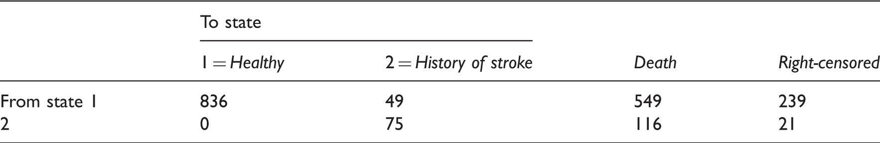
Originally, the MMSE was designed to screen for dementia. It contains questions on memory, language and orientation. Most of the questions are relatively easy for individuals with average cognition. MMSE sum scores below 10 are indicative of dementia. Individuals with scores in the range 25–30 are said to have normal cognitive functioning. Currently, the MMSE is also widely used to measure overall cognitive function. When the MMSE is applied in a population-based study such as CFAS, a large proportion of the observed MMSE sum scores will be in the range 25–30. In the data for men in Newcastle, the median of the MMSE sum score at baseline is 27.

MMSE scores are not always observed. There are 298 missing binary item scores in the records of 28 men. Nine men have a missing score for the five-category question.

3 Methods

In this section, the joint modelling framework is presented for latent growth trajectories and multi-state processes. First, the multi-state model is discussed, followed by the latent growth model part. The derivation of the joint posterior distribution concludes this section.

3.1 The multi-state model

This section presents the likelihood of the continuous-time multi-state model. The basic ideas can be found in Kalbfleisch and Lawless ³ and Jackson et al. ⁴ The formulation of the likelihood is different from that in Van den Hout and Matthews, ⁸ where an approximation with regard to exact death times was used. Transition probabilities in the likelihood are conditional on the current state and current values of risk factors. Commenges ¹³ uses the term partial-Markov to denote this kind of multi-state model since using the time-dependent risk factors implies that the process is not first-order Markov.

Let the interval-censored multi-state data be given by x ₁,…, x _N , where N is the number of individuals in the study. The trajectory of individual i is given by x _i  = (x_i1,…, x _{in i} ), where n _i is the number of observed states, and state x _ij  ∈ {1,…, S}, where j = 1,…, n _i indexes the consecutive times of measurement. Times of observation – not necessarily equidistant – are given by t_i1,…, t _{in i} , where t_i1 = 0, for all i, denotes the start of the study. For individual i, we have observed risk factor values w _i  = ( w _i1,…, w _{in i} ) at times t_i1,…, t _{in i} .

Let (t, u] denote a generic time interval. For a continuous-time multi-state model, transition probabilities p _rs (t, u) = P(x _u  = s|x _t  = r) are the entries of transition matrix P (t, u). Likelihood contributions are formulated using the transition matrices for the observed intervals, but the model itself is defined using intensity matrices which are matrices with transition intensities as entries. The transition matrix P (t, u) is derived from intensity matrix Q (t) by means of P (t, u) =  exp[(u − t) Q (t)], where exp[·] is the matrix exponential. ¹⁴ Off-diagonal entries of Q (t) not restricted to zero can be related to risk factors w by means of a log-linear model $\log [q_{\mathrm{rs}}(t_{\mathrm{ij}})]={\beta }_{\mathrm{rs}}^{\top }{w}_{\mathrm{ij}}$ . For example, a progressive three-state model where state 3 is the death state has vector β  = ( β ₁₂, β ₁₃, β ₂₃).

We assume a piecewise-constant multi-state model, where individual trajectories through the states are conditionally independent. For individual i, the likelihood contribution is

$p(x_i|\beta ,w_i)=P(x_{{\mathrm{in}}_i}|x_{i,n_i-1},\beta ,w_{i,n_i-1})\times \dots \times P(x_{i2}|x_{i1},\beta ,w_{i1}).$

This follows by conditioning on the first state, that is, by restricting P(x_i1| β , w _i ) = 1. The likelihood is given by $p(x|\beta ,w)={\Pi }_{i=1}^{N}p(x_i|\beta ,w_i)$ . See Appendix 1 for the construction of the likelihood of the three-state model that is used in the application and which takes into account exact death times and right-censoring and the end of the follow-up.

As implied by the above, we assume that given the current state and the current values of the risk factors, the distribution of the next state does not depend on the states visited before the current state. In addition, we assume that factor values are constant between consecutive observation times. Within each individually observed time interval (t _ij , t_i,j+1], this defines a time-homogeneous process. Using age as a piecewise-constant time-dependent risk factor, possible dependence of transition intensities on changing age is taken into account. ¹⁵

If there are no other risk factors besides age, the model for the intensities is given by log[q _rs (t _ij )] = β_rs.1 + β_rs.2Age(t _ij ). This can also be formulated as q _rs (t _ij ) = λ _rs exp[γ _rs Age(t _ij )], for λ _rs  > 0, which shows that the change of the intensities over time follows a Gompertz model with age as the time-scale.

3.2 Linear growth model for latent cognitive function

In our modelling, cognitive function is a latent time-dependent risk factor in the multi-state model. We assume that cognitive function is continuous and that the time-dependency can be described by a linear growth model. In the growth model, the function is represented by the variable θ.

For individual i with observation times t_i1,…, t _{in i} , let θ _i  = (θ_i1,…, θ _{in i} ). The growth model is given by

${\theta }_{\mathrm{ij}}={\eta }_{1i}+{\eta }_{2i}{t}_{\mathrm{ij}}+e_{\mathrm{ij}}\mathrm{\hspace{1em}\hspace{1em}\hspace{1em}}{\eta }_i=({\eta }_{1i},{\eta }_{2i})~\mathrm{MVN}(\nu ,\Sigma )\mathrm{\hspace{1em}\hspace{1em}\hspace{1em}}{e}_{\mathrm{ij}}~N(0,{\sigma }^2).$

That is, random effects η _i are multivariate normally distributed with unknown mean ν = (ν₁, ν₂) and 2 × 2 variance–covariance matrix Σ. The conditional distribution of θ _ij is normal with unknown variance σ². Random intercept η_1i is the value of θ _ij at the start of the study at time t _ij  = 0. Random slope η_2i reflects the change of θ _ij over time, where a negative value corresponds to a decline of ability over time.

Cognitive function is a latent variable as it cannot be observed directly but is measured by the MMSE. At every observation time, the MMSE consists of K = 25 binary items (questions) and one item with five ordered answer categories. IRT models are used to link the observed discrete values to latent function θ .

For individual i, the data for the binary response IRT model are given by y _i  = ( y _i1,…, y _{in i} ) with y _ij  = (y_ij1,…, y _ijK ). The probability of individual i answering binary item k correctly at time t _ij given item parameters a  = (a₁,…, a _K ) and b  = (b₁,…, b _K ) is defined using the probit model

$P(y_{\mathrm{ijk}}=1|{\theta }_{\mathrm{ij}},a_k,b_k)=\Phi (a_k{\theta }_{\mathrm{ij}}-b_k),$

(1)

where Φ(·) is the cumulative distribution of the standard normal. The probit model is well established in the IRT literature for cross-sectional binary response data. The logit model is sometimes used as an alternative, but in practice results for both models are similar. We prefer the probit model because it has a more simple implementation in MCMC.

For k = 1,…, K, parameter a _k is called a discrimination parameter and is the effect of a unit change in cognitive function θ on the success probability for item k. Parameter b _k is a difficulty parameter and is the effect on the success probability when θ = 0. Note that a large negative value of b _k corresponds to a relatively easy question.

Time-specific response data are assumed to be independent given time-specific cognitive function. This makes it possible to factorize the likelihood and we obtain

$p(y|\theta ,a,b)=\underset{i=1}{\overset{N}{\Pi }}\underset{j=1}{\overset{n_i}{\Pi }}\underset{k=1}{\overset{K}{\Pi }}P{(y_{\mathrm{ijk}}=1|{\theta }_{\mathrm{ij}},a_k,b_k)}^{y_{\mathrm{ijk}}}{(1-P(y_{\mathrm{ijk}}=1|{\theta }_{\mathrm{ij}},a_k,b_k))}^{(1-y_{\mathrm{ijk}})}.$

For the item with the five ordered response categories, we use the graded response model. ¹⁶ Let u _i  = (u_i1,…, u _{in i} ) denote the polytomous data for individual i. Given response categories 1 up to 5 (with the latter denoting the best score), the model has four ordered thresholds parameters d₁,‥, d₄. Together with the bounds d₀ = −∞ and d₅ = ∞, and the ordering d₀ < d₁ < d₂ < d₃ < d₄ < d₅, these thresholds define five segments on the real line. The graded response model written in cumulative normal response probabilities has parameters c and d  = (d₁, d₂, d₃, d₄), and is given by

$P(u_{\mathrm{ij}}=m|{\theta }_{\mathrm{ij}},c,d)=\Phi (c{\theta }_{\mathrm{ij}}-d_{m-1})-\Phi (c{\theta }_{\mathrm{ij}}-d_m),$

(2)

for m = 1,‥, 5. ¹⁷ The model defines the probabilities of the five answer categories. Parameter c is the discrimination parameter, and d is the difficulty parameter. As an example, when d₁ is a large positive number, the first segment from −∞ up to d₁ is large compared to the other segments. This implies that category 1 corresponds to a high probability and this reflects a difficult item. When d₄ is a large negative number, it is relative easy to obtain a score of 5. Notice that for an item with two categories, the thresholds would be −∞ = d₀ < d₁ < d₂ = ∞ and the graded response model reduces to the two-parameter (normal ogive) IRT model (1).

Fox ¹⁷ formulates this model for cross-sectional data, but – as above – given the conditioning on θ _ij , the same model can be used for longitudinal data. The likelihood is

$p(u|\theta ,c,d)=\underset{i=1}{\overset{N}{\Pi }}\underset{j=1}{\overset{n_i}{\Pi }}\sum _{m=1}^{5}P(u_{\mathrm{ij}}=m|{\theta }_{\mathrm{ij}},c,d)\delta (u_{\mathrm{ij}}=m),$

where δ(u = m) = 1 if u = m and 0 otherwise.

Analogous to the standard cross-sectional IRT model, we identify the growth model by fixing the scale of cognitive function θ . Note that for this variable, only differences are important – values considered at face value are not informative. The mean and the variance of θ are fixed to zero and one, respectively (sec. 4.4.2). ¹⁷

3.3 Posterior and prior densities

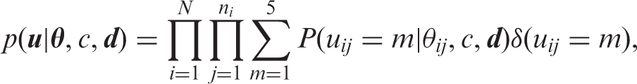
Bayesian inference is based on the posterior density of the model parameters. The posterior density is proportional to the likelihood of the data times the prior density of the model parameters. Ignoring manifest risk factors in the notation, the posterior of our model is given by

$p(\beta ,a,b,c,d,\theta ,\eta ,\nu ,{\Sigma }^{-1},{\sigma }^2|x,y,u)\propto p(x,y,u|\beta ,a,b,c,d,\theta ,\eta ,\nu ,{\Sigma }^{-1},{\sigma }^2)p(\beta ,a,b,c,d,\theta ,\eta ,\nu ,{\Sigma }^{-1},{\sigma }^2),$

(3)

where p( x , y , u | β , a , b , c, d , θ , η , ν, Σ⁻¹, σ²) is the overall likelihood of the multi-state data x , and MMSE data y and u . Given the model specification in Section 3.2, it follows that

$p(x,y,u|\beta ,a,b,c,d,\theta ,\eta ,\nu ,{\Sigma }^{-1},{\sigma }^2)=p(x|\beta ,\theta )p(y|a,b,\theta )p(u|c,d,\theta )$

The prior density for the parameters in (3) is given by

$p(\beta ,a,b,c,d,\theta ,\eta ,\nu ,{\Sigma }^{-1},{\sigma }^2)=p(\theta |\eta ,{\sigma }^2)p(\eta |\nu ,{\Sigma }^{-1})p(\beta )p(a)p(b)p(c)p(d)p(\nu )p({\Sigma }^{-1})p({\sigma }^2),$

where the conditional distributions of θ and η are specified in Section 3.2.

For the parameter β of the three-state model, we use a non-informative (improper) prior density: p( β ) ∝ 1. For the parameters of the growth model, the prior densities are given by

$\nu ~\mathrm{MVN}({\nu }_0,C)\mathrm{\hspace{1em}\hspace{1em}\hspace{1em}}{\Sigma }^{-1}~\mathrm{Wishart}({(\rho R)}^{-1},\rho )\mathrm{\hspace{1em}\hspace{1em}\hspace{1em}}{\sigma }^2~\mathrm{Inv}-\mathrm{Gamma}(\xi ,\xi ),$

see Gelfland et al. ¹⁸ These conjugate priors allow a straightforward implementation of the Gibb sampler that we use for the growth model. The choice of the hyper-parameters is discussed in the application. For the IRT model, we use non-informative prior densities for the item parameters: p( a ), p( b ), p(c), p( d ) ∝ 1.

4 Missing scores on test items

In CFAS, not all the MMSE questions are answered by all the individuals. Missing values are ubiquitous in statistical analysis, and we are not the first to point out that the Bayesian framework is very suitable for dealing with certain forms of missingness.

We will assume that values are missing at random, ¹⁹ i.e. the missingness does not depend on the missing value itself, but may depend on observed data. It will further be assumed that the parameters for the distribution of θ and the parameters for the distribution of the missing-data mechanism are a priori independent. With these two assumptions, the missing-data mechanism is assumed to be ignorable for Bayesian inference, (see definition 6.5). ²⁰ Given this assumption, Bayesian inference for the IRT model is relatively easy when item scores are missing. If, for example, for individual i at time t _ij , the value of y _ijk is missing, then the likelihood contribution for the items scores at t _ij can be formulated using the model for the items 1,…, k − 1, k + 1,…, K.

This flexible structure with respect to missing values is one of the reasons why we prefer to use an IRT model instead of using observed sum scores. The definition of a sum score is problematic when one or more item scores are missing.

Although we can estimate the model by ignoring the missing item scores, the MCMC method in the next section is easier to implement when we sample the scores along the way. In the MCMC algorithm, the missing scores are sampled first, after which the sampling of the model parameters proceeds as in the complete data case.

We illustrate the procedure for the binary response data. Given the probit model, latent cognitive function θ and item parameters a and b , sampling missing values is undertaken using Bernoulli trials. If at time t _ij , the binary value of y _ijk is missing, then we use a trial with success probability Φ(a _k θ _ijk  − b _k ). By sampling missing values in each iteration of the MCMC algorithm, the uncertainty with regard to the missing values is propagated into the sampling of the model parameters.

For a missing values of polytomous u _ij , values are sampled in a similar way using the multinomial distribution and parameters c and d .

5 Bayesian inference

MCMC methods are used to sample from the posterior distribution over the unknown parameters. The algorithm we use is a Gibbs sampler, ²¹ where each parameter is sampled conditional on the other parameters and the data. In case there is no closed form of the conditional probability distribution, Metropolis ²² or Metropolis–Hasting sampling ²³ is undertaken. This scheme is sometimes known as Metropolis-within-Gibbs although some authors dislike this term, see the discussion in Carlin and Louis, ²⁴ (sec. 3.4.4).

To summarize, data of individual i at time t _ij consist of observed states x _ij , binary response y _ijk for item k and polytomous response u _ij . Latent cognitive function is denoted as θ _ij . The parameter vector for the three-state model is β . Item parameters are a  = (a₁,…, a _K ) and b  = (b₁,…, b _K ), for the dichotomous item response model, and c and d  = (d₁,…, d₄) for the polytomous item response model. Parameters for the growth model are given by Ω = (ν, η , Σ, σ). Conditioning on manifest risk factors w is ignored in the following notation.

Sampling the parameters of the IRT model for the dichotomous response is undertaken using an auxiliary variable z  = ( z ₁,…, z _N ). This is a continuous representation of binary data y which makes it possible to formulate a Gibbs sampler. ²⁵ Corresponding to each y _ijk , we define the latent variable z _ijk which is normally distributed with mean a _k θ _ijk  − b _k and standard deviation 1. Value y _ijk  = 1 is observed when z _ijk  > 0, and y _ijk  = 0 is observed, when z _ijk  ≤ 0.

An innovative step in our Gibbs sampler is the sampling of θ . This parameter vector is sampled using a Metropolis step, where the sampling is informed by both the IRT data and the multi-state data. This illustrates the flexibility and the strength of MCMC.

Here, we enumerate the main steps of the Gibbs sampling, where conditioning on all other parameters is indicated by three dots, e.g., p( a |…). Details of each step and further references can be found in Appendix 2.

Sample missing binary scores $y_{\mathrm{ijk}}^{\text{mis}}$ from $p(y_{\mathrm{ijk}}^{\text{mis}}|\theta ,a,b)$ .

Sample missing polytomous scores $u_{\mathrm{ij}}^{\text{mis}}$ from $p(u_{\mathrm{ij}}^{\text{mis}}|\theta ,c,d)$ .

Sample z from p( z |…) ∝ p( z | θ , a , b , y ).

Metropolis sampling of θ . • A proposal distribution is specified by sampling from p( θ | z , a , b , Ω) ∝ p( z | θ , a , b )p( θ |Ω). • The vector θ sampled from the proposal distribution is re-scaled such that the resulting values have mean 0 and variance 1. • Sampled and re-scaled θ is the candidate for sampling from p(θ _ij |…) ∝ p(y _ij |θ _ij , a , b )p(u _ij |θ _ij , c, d ) p(x_i,j+1|x _ij , θ _ij , β )p(θ _ij |Ω).

Sample a from p( a |…) ∝ p( z | θ , a , b )p( a ).

Sample b from p( b |…) ∝ p( z | θ , a , b )p( b ).

Sample c from p(c|…) ∝ p( u | θ , c, d )p(c).

Sample d from p( d |…) ∝ p( u | θ , c, d )p( d ).

Sample Ω using a standard scheme for a linear mixed model, where θ is the response variable.

Sample β from p( β |…) ∝ p( x | β , θ )p( β ).

Posterior inference with regard to means, CIs and other derived quantities is based upon two chains, each with a burn-in of 5000 and an additional 15 000 updates. Convergence of the chains for the item parameters and the parameters for the growth model are assessed by visual inspection of the chains and by diagnostics tools provided in the R-package coda ²⁶ such as the convergence diagnostic by Geweke. ²⁷

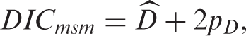
To compare models, we used the deviance information criterion. ²⁸ The DIC comparison is based on a trade-off between the fit of the data to the model and the complexity of the model. Models with smaller DIC are better supported by the data. The deviance of interest is the deviance of the multi-state model given by

$D(x,w,\beta ,\theta )=-2\log p(x|\beta ,w,\theta ).$

The DIC for the multi-state model is given by

${\mathrm{DIC}}_{\mathrm{msm}}=\stackrel{\wedge }{D}+2p_D,$

where $\stackrel{\wedge }{D}=D(x,w,E(\beta ),E(\theta ))$ and p _D denotes the effective number of parameters in the multi-state model. The latter can be estimated by $\overline{D}-\stackrel{\wedge }{D}$ , where $\overline{D}=M^{-1}{\sum }_{m=1}^{M}D(x,{\beta }^m,w,{\theta }^m)$ with m denoting the iterations in the MCMC algorithm. The DIC is therefore estimated by ${\mathrm{DIC}}_{\mathrm{msm}}=2\overline{D}-\stackrel{\wedge }{D}$ , where E( β ) and E( θ ) are estimated using the posterior means.

6 Application

The longitudinal MMSE data and multi-state data from the 925 men in CFAS in Newcastle will now be analysed. As stated before, in the three-state model, state 1 is the healthy state (no history of stroke), individuals in state 2 have had one or more strokes and state 3 is the death state. In the MMSE, there are 25 binary questions and one which is scored from 1 up to 5.

6.1 Estimation

Although the focus of the analysis is the three-state model, we briefly discuss the inference for the growth model for the MMSE data.

The choice of the hyper-parameters for the prior densities is ν₀ = (0, 0), C ⁻¹ = 0, ξ₀ = 1/100, ρ = 2 and R  = 10 I ₂, where I ₂ is the 2 × 2 identity matrix. This choice defines vague priors.

Posterior means and CIs for the parameters of the growth model are presented in Table 2. The negative posterior mean −0.036 for ν₂ which is the mean of the random slopes in the growth model concurs with our expectations. In the older population, if there is a change of cognitive function over a long time, then this will be a decline. The posterior mean 0.097 for Σ₂₂ reflects the heterogeneity that is present in the data with regard to these slopes. Interesting is also the negative posterior mean of covariance Σ₁₂, which means, for example, that a high intercept (high cognitive function) correlates with a small slope (less decline over time).

Table 2.

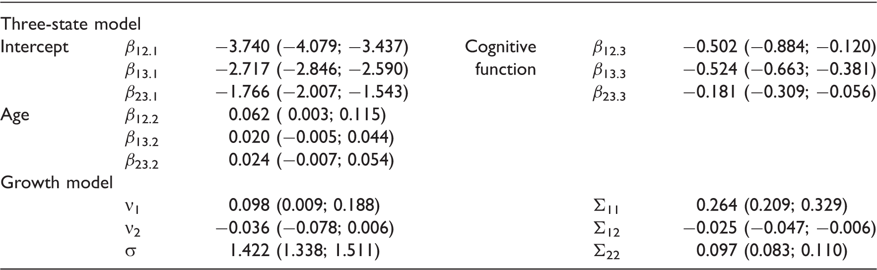
Posterior inference for model parameters with 95% CIs in parentheses

Three-state model
Intercept	β 12.1	−3.740 (−4.079; −3.437)	Cognitive	β 12.3	−0.502 (−0.884; −0.120)
	β 13.1	−2.717 (−2.846; −2.590)	function	β 13.3	−0.524 (−0.663; −0.381)
	β 23.1	−1.766 (−2.007; −1.543)		β 23.3	−0.181 (−0.309; −0.056)
Age	β 12.2	0.062 ( 0.003; 0.115)
	β 13.2	0.020 (−0.005; 0.044)
	β 23.2	0.024 (−0.007; 0.054)
Growth model
	ν1	0.098 (0.009; 0.188)		Σ11	0.264 (0.209; 0.329)
	ν2	−0.036 (−0.078; 0.006)		Σ12	−0.025 (−0.047; −0.006)
	σ	1.422 (1.338; 1.511)		Σ22	0.097 (0.083; 0.110)

We do not aim to investigate the effect of the individual items in the MMSE. Nevertheless, it is interesting to see that there is indeed variation in the item-specific characteristics. For the parameters for the binary items, see Figure 1. This illustrates why we are using an IRT model in the first place: assuming for instance that all questions are equally difficult is clearly incorrect (bottom part of Figure 1). Note that all difficulty parameters have a posterior mean smaller than zero. This reflects that for most people, the MMSE items are easy. And this is as expected since the MMSE is originally constructed to screen for dementia and the questions are relatively easy for the majority of the individuals in CFAS. The variation in the discrimination parameters (top part of Figure 1) shows that some items are better at discriminating individual cognitive function than others.

Figure 1.

Posterior inference for item parameters using boxplots. Discrimination parameters a in top graph, difficulty parameters b in the bottom one.

For the graded response model, the sampling of the threshold parameters d₁, d₂, d₃ and d₄ is depicted in Figure 2. The best way to sample threshold parameters has been a topic in the literature, (see sec. 4.3.4) ¹⁷ and the references therein. We used truncated normal distributions to generate new candidates in the Metropolis–Hasting step for d  = (d₁, d₂, d₃, d₄), see Appendix 2. Figure 2 illustrates that this sampling scheme works well. Numerical diagnostics for convergence as provided in coda ²⁶ all indicate good convergence.

Figure 2.

Monte Carlo Markov chains for the difficulty parameter vector 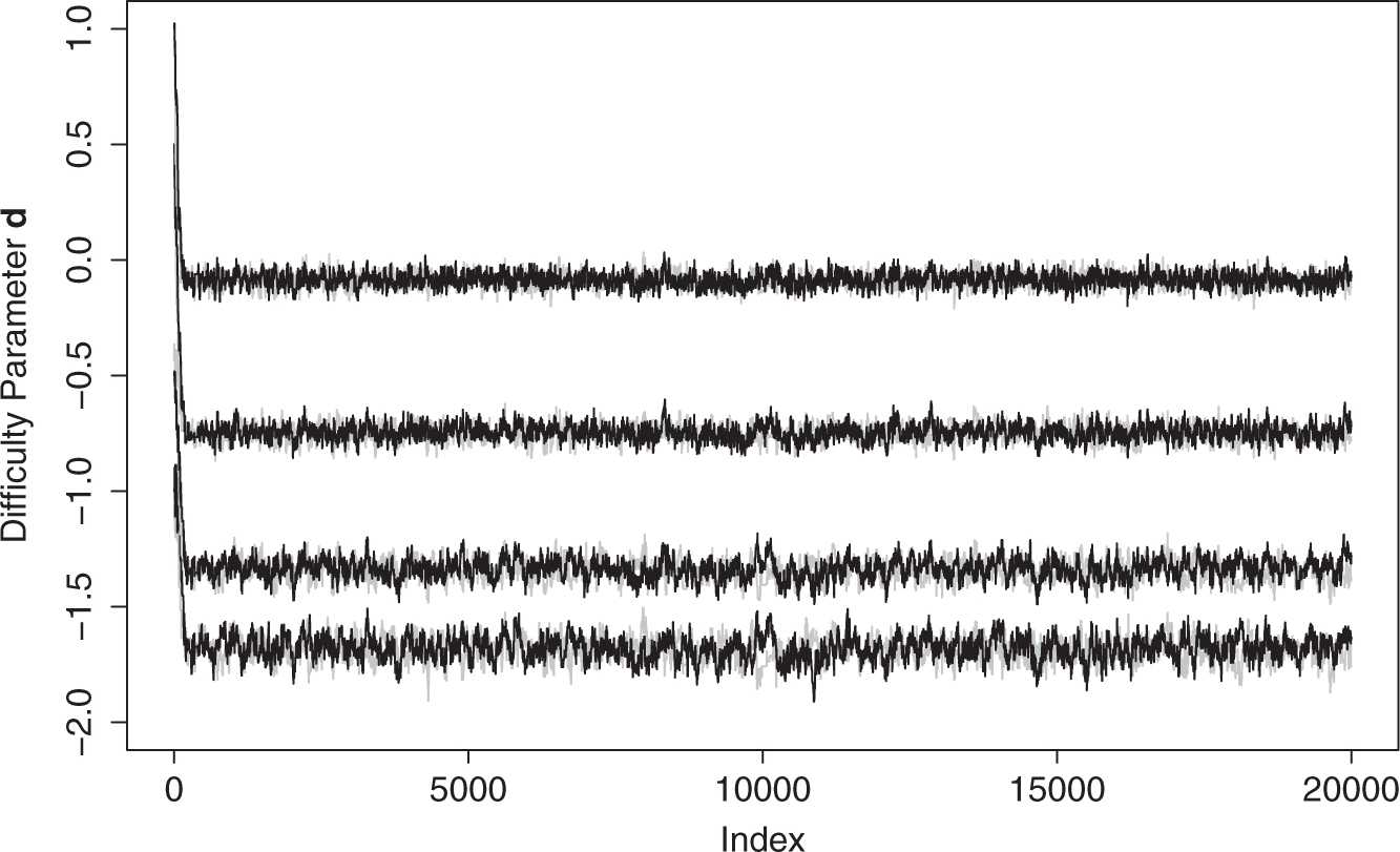d with thresholds d₁, d₂, d₃ and d₄. Burn-in included. Colours black and grey for the two set of starting values.

We now turn to the three-state model for stroke. The intensities are linked to age and cognitive function via the log-linear regression model given by

$\log [q_{\mathrm{rs}}(t_{\mathrm{ij}})]={\beta }_{\mathrm{rs}.1}+{\beta }_{\mathrm{rs}.2}\mathrm{Age}(t_{\mathrm{ij}})+{\beta }_{\mathrm{rs}.3}\theta (t_{\mathrm{ij}}),$

(4)

where Age(t _ij ) is the age midway through the interval (t _ij , t_i,j+1] minus 75 years, and θ(t _ij ) = θ _ij denotes latent cognitive function at time t _ij .

We start by examining whether adding age and cognitive function as risk factors provides a better model than the intercept-only model. The latter has DIC _msm  = 4825. The model with age but without cognitive function has DIC _msm  = 4777. Clearly, we get a better model by adding age. The final model, i.e. (4) with no restrictions, has DIC _msm  = 4680 which shows that taking cognitive function into account is worthwhile. Posterior inference for β in (4) is presented in Table 2.

The sign of the estimated effects of risk factors age and cognitive function are as expected: positive for age (getting older increases the risk of a transition) and negative for cognitive function (higher function is associated with a lower risk). Direct interpretation of the numerical results for the estimated effects is of limited use, see Section 6.4 for interpretation using estimated survival.

6.2 Goodness of fit

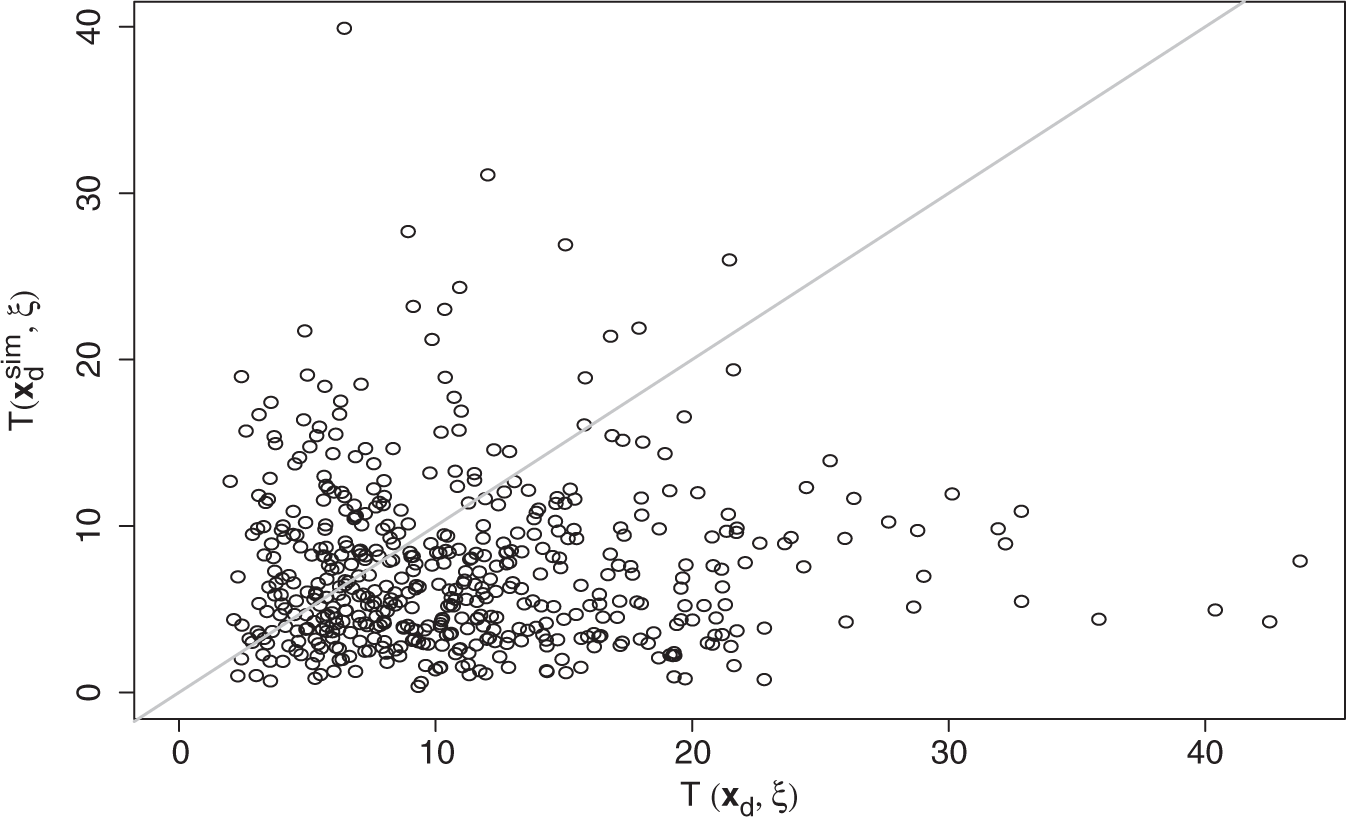
Model validation is undertaken by a posterior predictive model check. ²⁹ Validation is hampered by the interval censoring of the transitions between the healthy state and the state defined by a history of stroke. Death times are, however, observed during the follow-up. We propose to validate the model by comparing the deaths observed during follow-up with simulated deaths given the posterior distribution of the parameters. This does not capture all aspects of the three-state model, but nevertheless gives an idea of goodness of fit: if the simulated deaths differ significantly from observed deaths, then the model cannot be trusted.

We use a test statistic that depends both on observed deaths (say data x _d ) and on model parameters (denoted here by ξ ). For the time grids 0, 2, 4, 8, 10, 12, 14 and 16 in years since baseline, observed cumulative numbers of deaths at the grid points are given by O = (0, 121, 250, 465, 552, 620, 664, 665). Notice that the last figure is the sum of the numbers of transitions into the death state in Table 1. Let E be the corresponding vector with the cumulative numbers of expected deaths given model parameters. We define the statistic T( x _d , ξ ) = ∑ (O − E)²/E. The model check is the comparison of T( x _d , ξ ) with $T(x_d^{\mathrm{sim}},\xi )$ , where ξ varies according to its posterior distribution, and $x_d^{\mathrm{sim}}$ denotes simulated deaths given ξ . The estimate of the p-value is the proportion of simulations, where $T(x_d^{\mathrm{sim}},\xi )\ge T(x_d,\xi )$ . A p-value close to 0 or close to 1 means that the observed cumulative numbers of deaths are not very likely given the model. This would indicate a lack of model fit.

In the model check, given sampled ξ  = ( β , η ), deaths are simulated conditional on observed individual data (state and age) at baseline. At the grid points, age of individual i is known given age at baseline, and cognitive function θ _i is derived given time and sampled random intercept η_1i and slope η_2i. Simulation of the three-state survival conditional on baseline state can then be undertaken and simulated death times are monitored. In this simulation, the intensities change piecewise-constantly from grid point to grid point. The algorithm is a Gillespie ³⁰ algorithm, and is also used and explained in Van den Hout and Matthews, ¹⁵ where all risk factors are manifest.

We used 500 random samples from the MCMC for β and η , and obtained the p-value 0.30. Figure 3 depicts simulated $T(x_d^{\mathrm{sim}},\xi )$ and T( x _d , ξ ). With respect to observed deaths during the follow-up, the model seems to fit the data well.

Figure 3.

Posterior predictive model check. Comparing $T(x_d^{\mathrm{sim}},\xi )$ and T( x _d , ξ ) for 500 draws of ξ  = ( β , η ) from its posterior distribution.

6.3 Prediction

Although posterior means for β are informative with regard to the direction of the effect of a risk factor, for a practical understanding of the effect, it is more useful to investigate the predicted survival. Examples will be presented for three individuals: A, B and C, where the first two are hypothetical, and C is an individual in the study.

Consider the case of A who has had a stroke in the past. What is his survival curve (probabilities of not dying) for the next 15 years? According to our model, this depends on current and future cognitive functions. Assume that his current function is equal to the estimated population mean (η_A1 = ν₁). We consider baseline ages 65, 75 and 85. For each choice of baseline age, Figure 4 shows two survival curves conditional on assumptions with regard to the slope parameter in the growth model. For A, we assume that the slope is equal to the mean of its population distribution plus one standard deviation of that distribution ( ${\eta }_{A2}={\nu }_2+{\Sigma }_{22}^{1/2}$ ). The solid line is the estimated survival for A. Individual B is as A, except for his slope parameter which is equal to the mean of its population distribution minus one standard deviation ( ${\eta }_{B2}={\nu }_2-{\Sigma }_{22}^{1/2}$ ). The dashed line is estimated survival for B. The uncertainty in the graph (the 95% CIs) is with regard to the posterior distribution of β . Even though the CI-bands are quite wide, there is a clear and relevant difference in survival due to difference in future cognitive function.

Figure 4.

Prediction for men in state 2 at baseline, aged 65, 75 and 85 years old. Solid lines for survival if slope in growth model is equal to population mean plus one standard deviation, dashed lines for slope equal to population mean minus one standard deviation (thin lines for 95% CIs). Prediction of survival for selected individual who is in state 1 at baseline, aged 69 (grey lines if baseline state would have been 2).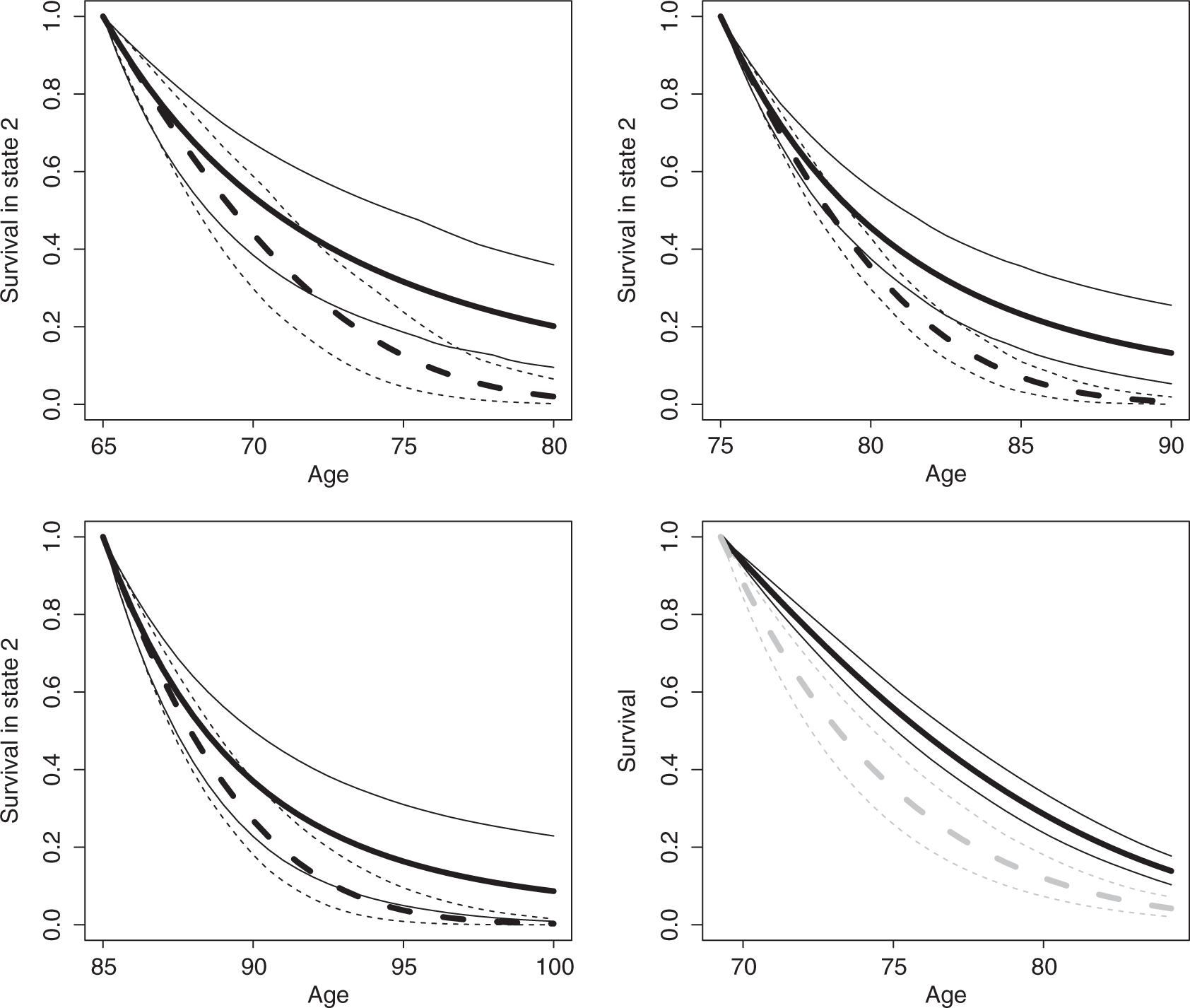

When it comes to prediction in practice, we would like to predict survival conditional on observed MMSE scores at baseline. Individual C has baseline scores y _C1 and u _C1. The posterior of θ_C1 = η_C1 is given by

$p({\eta }_{C1}|y_{C1},u_{C1},a,b,c,d,\nu ,\Sigma )\propto p(y_{C1}|{\eta }_{C1},a,b)p(y_{C1}|{\eta }_{C1},c,d)p({\eta }_{C1}|\nu ,\Sigma ),$

(5)

where p( y _C1|‥) and p( u _C1|‥) are likelihood contributions and p(η_C1|‥) is the density of the normal distribution with mean ν₁ and variance Σ₁₁. Maximizing (5) yields the most likely value of η_C1 conditional on the posterior means of the model parameters. This is called maximum a posterior (MAP) estimation.

C is an actual man in the data set. At baseline, he is 69 years old, has an MMSE sum score of 23 and has no history of stroke. The MAP estimate of baseline function is −0.670 which is in the lower part of the estimated population distribution with mean ν₁. Given baseline state 1 and assuming that the C's slope for the trend of cognitive function is the estimated mean ν₂ for the population, we can estimate the survival. The bottom right graph in Figure 4 depicts this survival.

We consider possible transition from state 1 to state 2. For C, the probability that he will be in state 2 after 15 years (estimated at 0.047) is less interesting than the probability of being in state 2 conditional on being still alive after 12 years. The latter is estimated at 0.047/(1 − 0.862) = 0.341 with 95% CI (0.244; 0.521), where the uncertainty is with regard to the posterior distribution of β , ν, Σ and σ. Given the conditioning on baseline function η_C1, we used

${\eta }_{C2}|{\eta }_{C1},\nu ,\Sigma ~N({\nu }_2+\frac{{\sigma }_{{\nu }_1}}{{\sigma }_{{\nu }_2}}\rho ({\eta }_{C1}-{\nu }_1),(1-{\rho }^2){\sigma }_{{\nu }_2}^2)$

where ρ is the correlation between intercept η₁ and slope η₂, derived from Σ. This conditional distribution follows from the distribution of Z₂|Z₁ = z₁ when both Z₁ and Z₂ are normally distributed, (see sec. 3.5.2). ³¹

7 Conclusion

This article presented an application, where a three-state model for stroke and survival encompasses a latent growth model for time-dependent cognitive function using longitudinal MMSE data. The cognitive function was included in the joint analysis as a time-dependent risk factor for transitions in the three-state model.

Adding the MMSE sum score as a non-deterministic time-dependent risk factor is not a problem with respect to the estimation of a multi-state model when we assume that the piecewise-constant approximation is reasonable. However, for prediction, we need a model for the time-dependent risk factor. A growth model with the MMSE sum score as response variable is problematic because the conditional distribution of the sum score is not normal, as the scale is discrete and there are ceiling effects. The binomial distribution is an alternative for the response distribution, but this distribution does not distinguish between the items (questions) that make up the sum score. It is only when IRT models are used that both the discrete nature of the MMSE and the item-specific characteristics are taken into account.

The presented growth model is an extension from the one introduced by Douglas. ³² Our model can deal with variation in time intervals between interviews and is more flexible due to the random-effects structure.

Both within the three-state model and the growth model, we have used assumptions that are commonly made. In the multi-state process, the transition probabilities are conditional on the current state and current values of risk factors. Using the time-dependent risk factors implies that the process is not first-order Markov. The process is also not semi-Markov because time spent in the current state is not taken into account. Another important assumption is that the piecewise-constant approximation captures the essential part of time-dependent risk factors. The IRT for cognitive function in the growth model assumes local independence (given the item parameters, scores are independently distributed) and time-independent item parameters. A posterior model check was used to validate the model in the application.

In the three-state model for the history of stroke, each individually observed interval (say (t _ij , t_i,j+1] for individual i) is modelled in the likelihood as a homogenous process, where values of risk factors at time t _ij are used to determine the distribution of the states at time t_i,j+1. It is because of this that we can say lower cognitive function is associated with a higher risk of stroke. Due to the piecewise-constant approximation, the model is not invalidated by the fact that a stroke often causes a drop in cognitive function. For example, if a stroke occurred within (t _ij , t_i,j+1] and there is a drop in function, then the decreased function will only play a role in the modelling of the next interval (t_i,j+1, t_i,j+2].

The use of MCMC methods ensures proper propagation of the uncertainty at the various levels of the model. Using a random-effects growth model, individual heterogeneity is taken into account. Given the general structure of the model, it can be extended easily, for example, with additional covariates in the growth model or in the multi-state model. Possible sub-models may also be of interest. For example, if there is no MMSE information available, the growth model can be dropped from the overall model, and θ _ij can take the role of a frailty which takes into account unobserved heterogeneity with regard to the risk of ill-health or death.