Understanding the root cause(s) of nonlinearities in near infrared spectroscopy

Abstract

NIR process monitoring and NIR hyperspectral video generates a deluge of non-selective spectral data, information-rich but per se useless. This paper demonstrates how interpretable data modelling can lead to simpler and better use of such NIR Big Data: A set of simple powder mixtures of the main constituents in wheat flour were measured by NIR transmission under different measurement conditions. Their absorbance spectra were submitted to multivariate calibration for predicting the protein content, by standard chemometric calibration by PLS regression. A reasonable calibration model was obtained, but it was unexpectedly complex and not robust.

However, closer inspection the PLS regression subspace showed a surprising structure. This allowed us to identify the problem: Non-additive, strongly overlapping light scattering and light absorption effects in the NIR absorbance spectra.

Based on this insight, a pragmatic, but causal preprocessing model was set up and iteratively optimized for predictive ability. This nonlinear optimized extended signal correction (OEMSC) separated and quantified the main physical and chemical sources of variation in the spectra. The preprocessing greatly simplified the NIR spectra and their quantitative calibration and prediction.

The body of work produced by Professor Harald Martens on multivariate analysis and near-infrared spectroscopy spans almost 50 years. His contributions to the chemical, biological, food science, agriculture and other industrial fields are important for their insights into both their understanding of the basic science and for providing pragmatic solutions for future applications. Professor Martens is a Fellow of Near Infrared Spectroscopy. He was elected by the International Conference of Near Infrared Spectroscopy in 2015. In Part 1 of this series: Notes on the use of Modern Multichannel Measurements, Harald helps us understand the underlying root causes of nonlinearities of near-infrared spectra using classical chemistry, physics and an innovative chemometric tool developed by Harald and colleagues; Optimized Extended Multiplicative Signal Correction (OEMSC).

Introduction

Now society has an urgent need for tools to let humans understand the information hidden in Big Data. Continuous, high-speed multiwavelength diffuse spectroscopy creates Big Data. Can our field contribute something towards a more humane, robust and efficient artificial intelligence? This author thinks so, based on the way NIR culture has been using interpretable data-driven modelling for several decades, not even knowing that we were using “machine learning”.

Here is an illustration. The light that we see is dominated by two major phenomena: Chemical light absorption is mainly caused by molecules “killing” different amounts of light at different wavelengths, leaving the rest to reach our eyes and cause colour sensation. Physical light scattering is caused by local variations in the refractive index that force the light to change direction. Think of air bubbles in whipped scream, oil droplets in mayonnaise or protein particles in hard-boiled egg.

In fact, most of what we look at is affected by both chemical light absorption and physical light scattering. For humans and animals that is fine: Without light scattering, we would have been transparent. Without light absorption, life would have been grey.

But since chemical light absorption and physical light scattering are very different natural phenomena, their effects on light measurements carry very different types of information. Hence, one given spectrophotometer or hyperspectral camera system can be used for quantifying a wide range of properties. As the readers of this journal very well know, the variations in one single measured spectrum can be converted into a number of different information types, depending on what it has been calibrated for.

Several different chemical compounds may be characterized with respect to their concentration and sometimes even their molecular state. Large groups of naturally correlated chemical compounds may also be quantified. Several different physical variation types may likewise be observed from the light scattering properties, ranging from surface and particle-size and -distribution to simple assessment of sample thickness.

For optimal instrument output, the way the different chemical and physical variations affect the measured spectra need to be modelled mathematically – not perfectly, but with sufficient realism. Some of these causes for spectral variation are known and of interest; others are known, but just a nuisance, and many are simply of unknown type.

In general, all spectral variation types that overlap spectrally with the variations of real interest need to be handled – either kept constant or modelled and thus compensated for mathematically in the multivariate calibration process. To be modelled, their variations must either be observed within the calibration sample set or described based on prior knowledge. Either way, it is advantageous to understand which variations need to be modelled and how.

Multichannel measurements, e.g. from a high-speed scanning spectrophotometer or a hyperspectral video-camera, certainly represent Big Data. But instrument calibration is risky business if performed according to the paradigm “just get yourself some Big Data and apply Artificial Intelligence (AI)/Machine Learning (ML)”. Today, this unfortunate tradition is under heavy attack, both ethically, legally and economically. The new buzzword is “Explainable AI” (XAI).

This paper will show how precise, but highly confusing and non-selective diffuse spectroscopy can be converted into more accurate, precise and understandable information, based on chemometric methods. This will be illustrated using a small set of “on purpose dirty” spectral measurements that Jesper Pram and I made for didactic purposes about 20 years ago at U Copenhagen, in the chemometrics group that prof. Lars Munck originally established there.

The data analytic problems and the solutions are rather generic. Therefore, in case the readers or their colleagues might find them useful also for XAI/ML and Big Data in general, they will mainly be described in non-technical terms.

Experimental

The present didactic data set ¹ concerns a “classical NIR” topic, protein quantification in dry wheat flour by high-speed NIR transmission spectroscopy. A total of 100 absorbance spectra were collected in the range of 850–1048 nm using an Infratec 1255 Food and Feed Analyzer (FossTecator, Höganäs, Sweden) fitted with a standard sample holder for five cylindrical cuvettes. Five different flour mixtures were each measured 20 times under 20 different experimental conditions. For linearization, the measured transmittance T was converted into absorbance A by the usual A = log(1/T). More technical information about the experiment is given in Appendixes 1 and 2.

The instrument itself is known to give very precise and accurate measurements. And NIR measurements are fast and simple: Virtually no sample preparation is required – just put the powder into the sample holder with a glass bottom, put on a glass top and measure how much light is transmitted through the sample at the different wavelengths. Virtually no sample preparation, and very simple measurements. That is the charm of NIR.

Results and discussion

Figure 1 shows the 100 measured absorbance spectra obtained. Why do these simple two-component mixtures give so unexpectedly “dirty” spectra? How can they be robustly converted into “clean” information?

Figure 1.

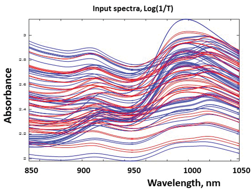
Multichannel instruments: Enough data to confuse the human eye! Five different chemical compositions, each measured under 20 different conditions. Blue = 60 spectra representing 0%, 50% and 100% gluten, are to be used as training data for model development. Red = 40 spectra representing 25% and 75% gluten, to be used as independent test set.

At least the “dirty” data make some sense: The absorbance spectra display several different “chemical” absorbance maxima, as expected for mixtures of constituents known to have peak-shaped absorbance spectra.

The varying measurement conditions appear to affect the spectra strongly. How detrimental are these unknown variations, and how should we deal with them?

With sufficiently informative calibration data, “modern machine learning,” e.g. an artificial neural net or a support vector machine, could probably have extracted the desired chemical information from these input absorbance spectra in the calibration sample set. But it is important to maintain control over the calibration process, for unexpected errors may have occurred. Moreover, the number of calibration samples is very limited (only three chemical compositions).

So we choose a simple, linear calibration model, and estimate the calibration model parameters by a traditional, easily validated chemometric calibration technique, the cross-validated Partial Least Squares Regression ² (PLSR). Figure 2 shows the resulting prediction ability to be reasonably good, although it is not perfect.

Figure 2.

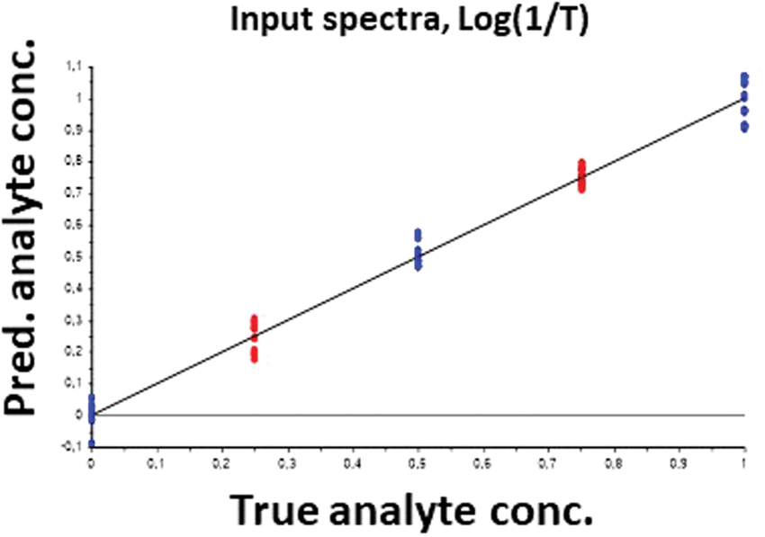
Black box operation: Checking THAT the “machine learning” worked: Predicted vs. known levels of the analyte (the protein concentration for the three “known” mixtures (blue) and the two “unknown” mixtures not involved in the machine learning process itself (red).

Satisfied with that, we now go to the simplest type of XAI: We want to know HOW the machine learning solution converts the many measured channels X into predictions of protein concentration y. That is shown in Figure 3, in terms of the so-called regression coefficient spectrum b that summarize the PLS Regression model. A linear combination of high spectral values around 910 and 1030 nm and low levels around 860 and 990 nm is seen to contribute to the prediction of high levels of y.

Figure 3.

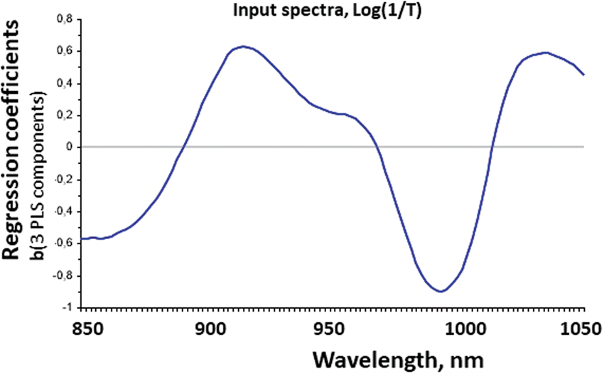
The beginning of XAI: Checking HOW the “machine learning” predicts y from X. The regression coefficient spectrum $\widehat{\mathbf{b}}$ for y in the linear PLSR predictor $\widehat{\mathbf{y}}={\widehat{\mathbf{b}}}_0+\mathrm{X}\times \widehat{\mathbf{b}}$ , using three PLS components (offset ${\widehat{\mathbf{b}}}_0$  = 0.315).

Similar model summaries may be obtained from a wide range of multivariate statistical regression or ML tools. This information is much better than nothing. At least we see how different aspects of the measurements are balanced against each other for the prediction, and gross mistakes may sometimes be discovered.

But alas, but it does not give meaningful explanation about WHY the different input variables are combined this way in this application. Without that, we are still in the dark as to how reliable and robust this result it.

To get to a deeper level of understanding, we employ a characteristic aspect of the chosen ML method, the PLSR, ² namely the low-dimensional subspace it generates to describe the most relevant variation patterns in the spectra. Subspace regressions (PLSR, Principal Component Regression PCR, etc.) replace the many (K) input variables in X by a small set of “supervariables” or “components” from X (linear combinations, after mean-centering and scaling).

The PLSR version of subspace regression searches for orthogonal components that explain maximal X/y covariance. These are then used for modelling y. The best number of subspace dimensions (components) is often determined by so-called cross-validation within the calibration set. Then the model is applied to new samples to predict y from X.

Models with 1, 2 or 3 components here explained 68, 95 and 98% of the cross-validated variance in y in the calibration set, respectively. In the independent test set, with very different y-levels, they explained 18, 88 and 97% variance in y, respectively. So in both cases, the three component-solution gave the “best” predictive performance.

However, this “best” solution has two troublesome aspects:

Given that the present samples were just mixtures of two constituents whose sum was 1, we expected to need only one component. But the 1-component solution explained only 18% of the Y-variance in the test set. So why do we need three components? What are the other two sources of variation in the spectra?

The third component picked only up a very small spectral variation pattern (0.005% of the variance in X). So while it appeared necessary for predicting y, the three-component model is probably not robust – it may be very sensitive to increased measurement noise. But the two- or one-component models simply are not good enough. Que faire?

Understandable machine learning with an eye for causalities

If we could find out what it is that plays havoc in our NIR absorbance spectra, then we could model it explicitly and thereby hopefully develop a more robust calibration model from the same data.

Subspace regression methods give us a unique advantage: We can inspect the first few subspace dimensions graphically, getting insight into what is going on in the data. Perhaps we can thereby get ideas about what has caused the variations, and how they can be modelled more efficiently. And then we can test these ideas.

Inspecting the first two PLSR components (Figure 4, linear combinations of the spectra in Figure 1), we see that the five mixture samples showed an intriguing variation pattern: The different measurement conditions within each of the three calibration mixtures (blue) and two test mixtures (red) form distinct lines, one for each protein percentage tested. Each line ranges from low (top, right) to high powder compression. Their extrapolations meet in a featureless offset spectrum.

Figure 4.

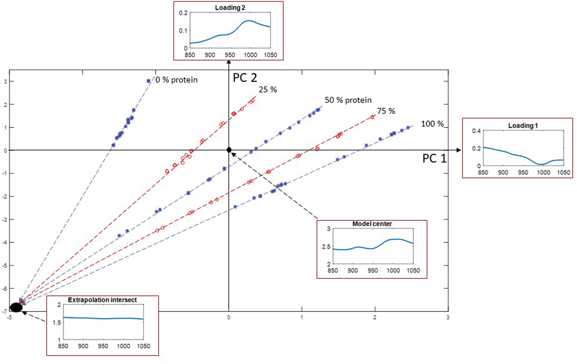
TRYING to see WHY: Searching for clues about the spectral variations in Figure 1. The score space of the first two PLSR components around the model center, with their spectral definitions.

Armed with this new spectral insight, we now build a pragmatic, semi-causal preprocessing model and fit it to each spectrum, by a method is called Extended Multiplicative Signal Correction EMSC. ³ The EMSC allows a simultaneous correction for both additive and multiplicative interferences. The additive correction can, e.g. reduce unwanted chemical absorbance interferences according to Beer’s Law, as well as lamp intensity variations and other baseline variation, while the latter correction can reduce unwanted variations in optical path length according to Lambert’s Law.

Building in chemical background knowledge, the EMSC has been applied to these present data. ¹ We recently used the EMSC as preprocessing of very large amounts of hyperspectral video data in the VNIR ⁴ and SWIR ⁵ ranges, respectively, to monitor the drying of wood in terms of known and unknown chemical and physical variation types.

In order to make the EMSC model easier to set up in practice, the author modified it into the present Optimized EMSC (OEMSC ⁶ ). A new, abstract dimension was added to the EMSC model and fitted iteratively to a given set of calibration data by non-linear simplex optimization, minimizing the prediction error in the calibration samples’ y-data. Once optimized, the OEMSC model is then applied also test samples etc.

Figure 5 shows that the predictive ability improved after the OEMSC pre-treatment. Moreover, with after pre-treatment the PLSR calibration model only required one single PLS component, as expected for these mixtures of two powders.

Figure 5.

Checking THAT the new pre-processing has improved the “machine learning” (PLSR with only 1 component), compared to Figure 2: Predicted vs known levels of the analyte (the gluten concentration) for the three “known” mixtures (blue) and the two “unknown” mixtures not involved in the machine learning process itself (red).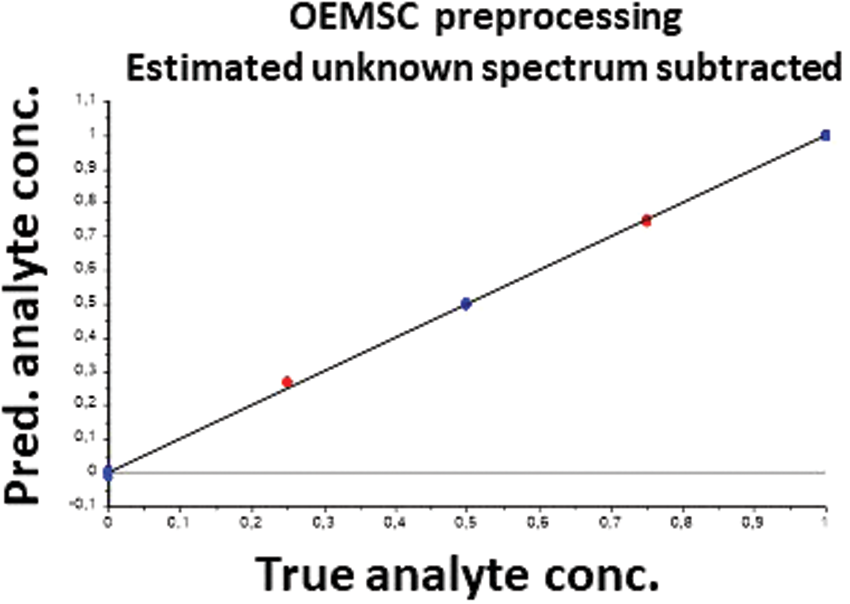

Figure 6 shows how the PLSR combined the preprocessed absorbance from the different wavelength channels to predict the protein content, in terms of the regression coefficient spectrum $\widehat{\mathbf{b}}$ estimated using 1 PLS component. It is quite different from that in Figure 3. This illustrates that the model summary $\widehat{\mathbf{b}}$ like the one in Figure 3 may be difficult to interpret spectroscopically.

Figure 6.

Checking HOW the “machine learning” predicts y from X after the OEMSC preprocessing. The regression coefficient spectrum 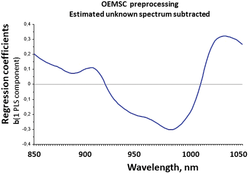$\widehat{\mathbf{b}}$ for y in the linear PLSR predictor $\widehat{\mathbf{y}}={\widehat{\mathbf{b}}}_0+\mathrm{X}\times \widehat{\mathbf{b}}$ , using only 1 PLS component.

For the results in Figure 5 and 6, the new, abstract EMSC model dimension has been optimized to give preprocessed spectra with optimal y-prediction after it has been subtracted.

Why had the predictive ability been improved and the model complexity been reduced by the OEMSC preprocessing? Figure 7 (left side) shows what this version of the OEMSC preprocessing had done to the 100 spectra in Figure 1.

Figure 7.

USING the new insight: The same 100 spectra as in Figure 1, but after having applied two alternative versions of the OEMSC. Left: OEMSC optimizing and subtracting a new spectral model dimension found. Right: OEMSC optimizing, but not subtracting a new spectral model dimension found. Each curve represents one of the five analyte levels 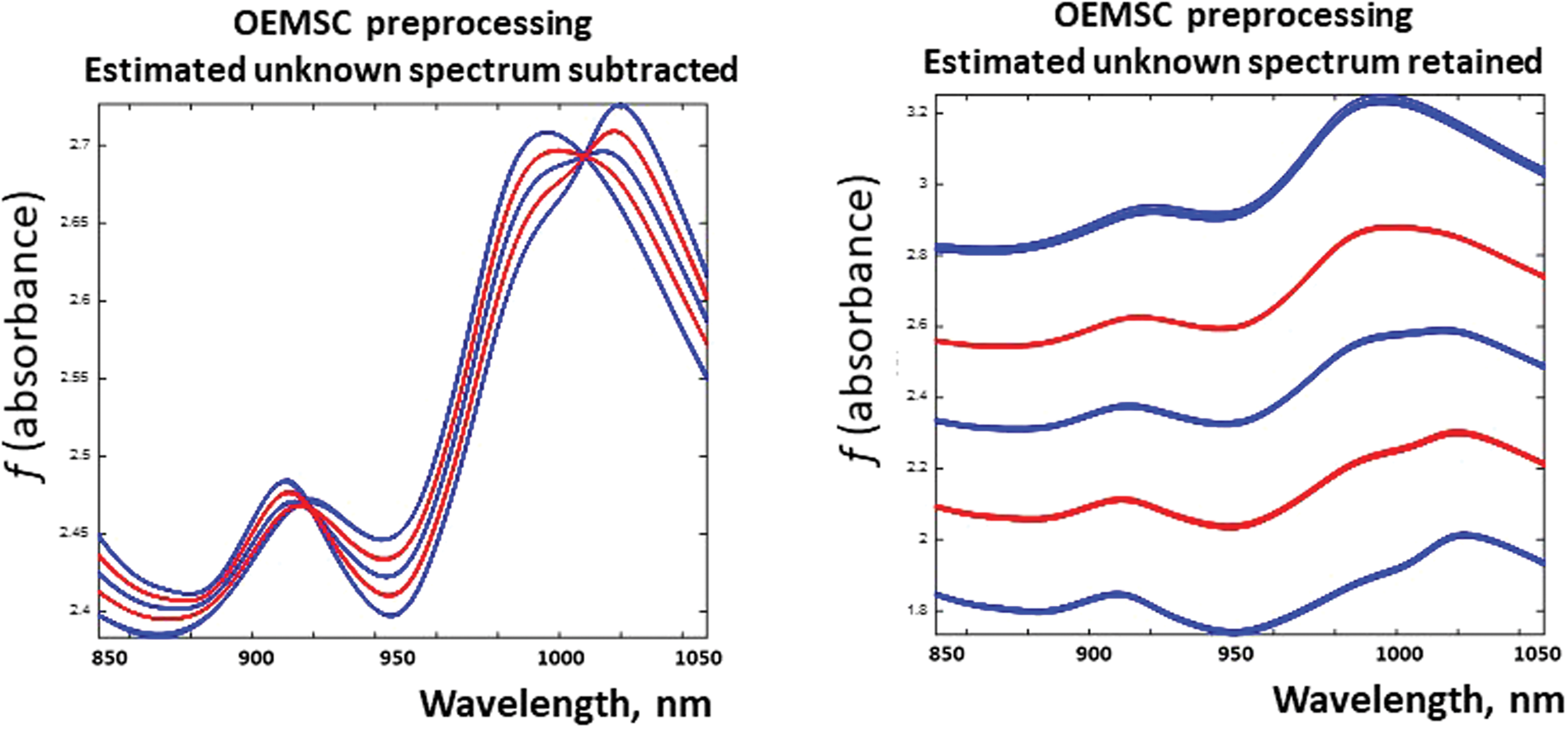y (gluten fraction) and contains 20 individual sample treatments.

The effect of light scattering appears to have been eliminated, leaving only absorbance information in the preprocessed NIR spectra. The simplified regression coefficient $\widehat{\mathbf{b}}$ in Figure 6 just reveals how the spectra change when the protein fraction increases.

However, the OEMSC can be used in different ways for the same data. In the right subplot the OEMSC has instead been optimized to give preprocessed spectra with optimal y-prediction without being subtracted (Figure 7, right side). Method details⁶ are explained in the Appendix.

Again, a single-component PLSR model gave best prediction, and the predictive improvement (not shown here) was very similar to those in Figure 5. But now a systematic variation in light scattering is retained in the preprocessed data. The difference in appearance between the two OEMSC solutions in Figure 7 indicates that the two causal constituents, wheat protein and wheat starch powders, differed both in chemical absorbance signature and in physical light scattering. Hence, in this case, both the chemical absorbance and the physical light scattering could in principle be used in a final calibration model.

Is the beneficial effect of the OEMC only relevant for such simple calibration examples? That remains to be seen, but here is the author's assessment:

The EMSC model can be extended to successfully handle quite complex variation types.^4,5 The OEMSC just extends the EMSC model with one more dimension and should therefore also be able to work for more complex systems. On the other hand, this small example concerned diffuse transmittance measurements. The lessons learned may be expected to generalize also for diffuse transflectance. But for diffuse reflectance the OEMSC may have to be modified to accommodate the effects of specular reflection and very short optical path length there.

In summary – diffuse multichannel spectroscopy of intact samples can give confusing data, and lots of them. Multivariate calibration by some sort of data-driven modelling can reduce some of the confusion. If a subspace-type regression is used in this “machine learning,” e.g. the PLSR, then a graphical inspecting of the regression subspace may allow us to discover why the spectra vary more than anticipated. This new insight can help us formulate better spectral pre-treatment models. In the present case, this understanding allowed us to formulate a mathematical description of the combined light absorbance/light scattering problems, and to use this in a preprocessing that improve the sanalyte quantification prediction.

In that sense, the subspace modelling, as practiced in chemometric analysis of diffuse NIR spectra, offers generic tools for hybrid data-and-theory driven modelling. These can be used for people to discover causes of wanted and unwanted patterns in e.g. quantitative Big Data, within XAI.