A 2500-year record of relative sea-level change at Gress,Isle of Lewis,northwest Scotland using salt marsh sediments

Abstract

Relative sea-level (RSL) changes in mid-latitude regions commonly reflect complex interactions between global ice-sheet melt, ocean dynamics and glacial isostatic adjustment (GIA), yet high-resolution Late-Holocene records from critical transitional zones near former ice-sheet margins remain sparse. Northwest Scotland, situated near the periphery of the former British-Irish Ice Sheet (BIIS), offers insights into spatially variable RSL trends driven by GIA and regional ice-mass loss, but existing reconstructions are limited in temporal continuity or geographic coverage. Out study addresses this gap by presenting a 2500-year RSL reconstruction from salt marsh sediments at Gress, Isle of Lewis—a location sensitive to BIIS-related lithospheric adjustments. Using a multi proxy approach (lithology, sedimentology, diatom biostratigraphy, and Accelerator Mass Spectrometry ¹⁴C dating), we produced a high resolution RSL record. We found challenges with diatom-based transfer functions due to poor modern analogues in the training set. This led to a qualitative visual assessment of fossil assemblages to reduce paleomarsh surface elevations (PMSEs). Consistent PMSEs show that the marsh surface elevation is a consequence of the rate of sediment accumulation, keeping up with modelled GIA uplift rates. A (1.2 ± 1) m (2σ) RSL rise throughout the core’s 2500-year record was observed, with a slight accelerated sea level rise post-AD 950. RSL rise at ~AD 1300 likely exceeded the background Late-Holocene fall rate (−0.2 mm yr⁻¹) until present. It proved challenging to distinguish the effects between barystatic sea level change and local influence on RSL patterns at our site. Any sea level acceleration in the last two millennia remains statistically indistinct in these sediments. Comparison with regional records highlights pronounced spatial heterogeneity in RSL trends, underscoring the influence of local GIA variability.

Keywords

sea level salt marsh paleoenvironmental reconstruction visual assessment diatoms Scotland

Introduction

Reconstructions of past relative sea-level (RSL) variations can inform us about elements of the Earth climate system, and response to forcings and in turn, aid in refining future sea-level predictions. Paleo sea level records capture the impacts of mass balance changes of polar ice sheets and mountain glaciers, and the associated solid Earth response, alongside ocean-atmospheric processes (Dutton et al., 2015; Milne and Shennan, 2013). As a result, they can help us interpret climate dynamics across warmer and colder periods in history (Dutton and Lambeck, 2012; Kopp et al., 2009). Previous work has demonstrated the importance of better constraints on polar ice sheet mass flux in both physical and semi-empirical models which help to predict future sea levels (Goelzer et al., 2020; Lecavalier et al., 2014; Mitrovica et al., 2011). Considering the anticipated role of Greenland and Antarctic ice sheets as primary contributors to rising relative sea levels under anthropogenic warming, paleoclimate signatures in RSL records can serve as crucial insights to potential polar ice sheet behaviour in a warming climate (Dutton et al., 2015).

RSL can be affected by global, regional and local processes, primarily by changes in ocean mass balance (barystasy) and vertical land-level change (isostasy). The combined effects of these processes vary both spatially and temporally (Horwath et al., 2022; Li et al., 2024; Milne and Shennan, 2013; Purkey et al., 2014). In higher mid-latitude northern hemisphere locations, regions near to former ice sheet centres (termed near-field) experience deglacial and Holocene RSL changes predominantly due to glacial isostatic adjustment (GIA) (Clark et al., 1978; Kemp et al., 2013). At lower mid-latitudes (intermediate-field regions), deglacial RSL is largely controlled by barystatic sea-level change (Clark et al., 1978; Kemp et al., 2013; Khan et al., 2015), which is RSL change due to water mass moving from land or atmosphere to or from ocean bodies (Gregory et al., 2019). As both these effects superimpose each other across various locations and timescales, there is no single pattern of RSL change applicable in mid-latitude locations (Kemp et al., 2013).

The United Kingdom (UK) is an ideal location to study the various drivers of sea-level change. First, coastal sites in the UK contain sediment archives and landforms that record changing sea level since the Last Glacial Maximum (LGM; Edwards, 2006; Lloyd et al., 2013; Shennan et al., 2018). Second, the isostatic responses to the formation and melting of the British and Irish Ice Sheet (BIIS), which once covered most of Ireland and northern Britain, produces spatially varying RSL (Bradley et al., 2011, 2023; Shennan et al., 2018; Smith et al., 2000, 2019). GIA effects in the UK follow a largely north-south pattern (Figure 1), with the north experiencing 0–2 mm yr⁻¹ vertical land motion and the south 0 to −1.4 mm yr⁻¹ vertical land motion over the Late-Holocene (last 5000 years) (Bradley et al., 2011; Gehrels, 2010; Shennan et al., 2012). An updated global GPS data set developed to test and improve modelled GIA uplift rates also show similar north-south trends from 2005 to 2015, with the north showing pronounced crustal uplift rates of more than 5 mm yr⁻¹ while the central and south shows slower uplift rates of between 0 and 5 mm yr⁻¹ (Schumacher et al., 2018). Third, marine-terminating ice streams resulted in rapid deglaciation in the region (Patton et al., 2013), causing localized RSL fall in the immediate vicinity of the deglaciated regions. Fourth, much of the UK lies along the margin of the Fennoscandian ice sheet, which subsequently experienced proglacial forebulge collapse (Shennan et al., 2018). By reconstructing high-resolution Holocene RSL records at various locations from ice loads, we can better understand the spatial distributions of RSL patterns and its potential driving factors over centennial to millennial timescales.

Figure 1.

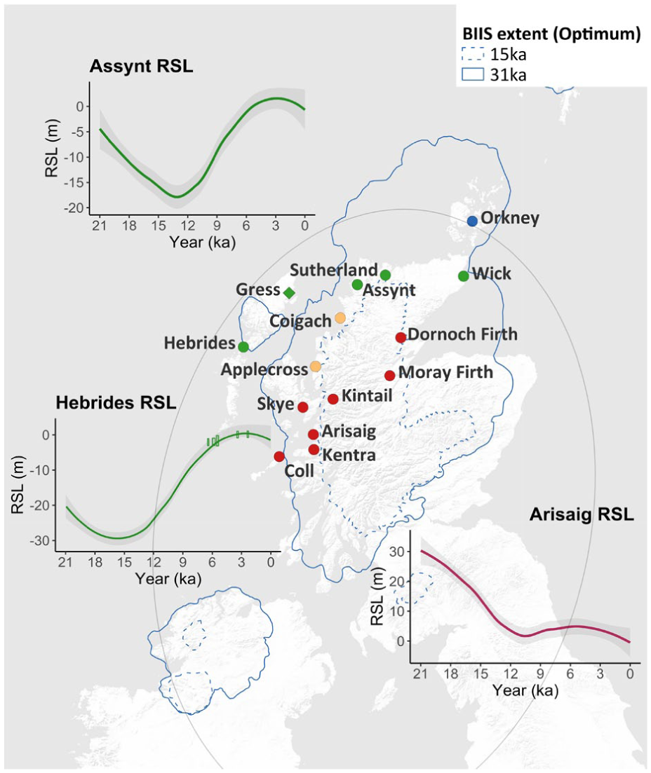
Existing RSL reconstruction sites in UK, with optimum BIIS extents (15 and 31 ka) plotted using data from PANGAEA (Clark et al., 2022). A loess smoothing function of 95% confidence interval was applied to the GIA-modelled RSL data from the online visualization tool PALTIDE (Bradley et al., 2011; Scourse et al., 2024; Ward et al., 2016). The colour scheme classifies sites with similar RSL histories following (Shennan et al., 2018). Field site of this study (Gress) is marked with a diamond. Key RSL reconstructions from this region are plotted as insets (Assynt, Hebrides, Arisaig). For the Hebrides inset plot, RSL reconstructions from (Jordan et al., 2010) were plotted as rectangles. The grey oval depicts the RSL zero isobase contour for the region, defined as the contour of zero GIA-driven present-day RSL rates, with areas outside the contour representing positive rates and vice versa (Bradley et al., 2023). The RSL zero isobase contour was adapted from Figure 9a in (Bradley et al., 2023).

In Scotland, RSL pattern changes are controlled by GIA effects due to both deglaciation of the British-Irish Ice Sheet (BIIS), and the outermost influence from the Fennoscandian Ice Sheet (Bradley et al., 2023; Hamilton et al., 2015; Smith et al., 2000, 2019). In northwest Scotland, only three Holocene RSL records exist – one proximally close to our study site focussed on the early-Mid-Holocene (Jordan et al., 2010) and two focussed on the Late-Holocene (Barlow et al., 2014). During the Mid-Holocene, RSL rose rapidly in Harris, Outer Hebrides, reaching ~2.0–4.0 m below present Mean High Water Spring Tide (MHWST) by ~6200 BP, followed by fluctuations until stabilization after ~3100–2100 BP (Jordan et al., 2010). Mid-Late Holocene RSL variability suggests secular sea-surface changes due to isostasy rather than tectonic activity, as no differential isostatic uplift was detected between nearby sites (Jordan et al., 2010). The two Late-Holocene RSL reconstructions show stable to slightly falling RSLs (±0.4 m) at Loch Laxford and Kyle of Tongue during the last 2000 years, with evidence of a slight rise in the last century (Barlow et al., 2014). The two field sites are located along the NW coast and within the thinner region of the paleo ice load which had a maximum extent up to the continental shelf. The scarcity of RSL records in northwest Scotland result in a poor understanding of GIA or other driving factors of RSL in this region. This spatial difference must be better understood in the context of the interplay of drivers of local RSL in the region.

In this paper, we develop a RSL record further from the Last Glacial Maximum ice load centre, where barystatic sea level is likely to be more dominant, but where there is still sufficient sediment supply to develop a continuous record to assess the spatial patterns in Holocene sea level around northwest Scotland. We produce a record from a previously unstudied salt marsh at Gress on the eastern coastline of the Isle of Lewis in the Outer Hebrides, at a location near to the edge of BIIS (Bradley et al., 2023; Shennan et al., 2018; Smith et al., 2019). Here we employ a multi-proxy approach to quantify Late-Holocene RSL changes at Gress across the last two millenia. Our reconstruction from the island offshore of northwest Scotland supplements existing RSL records in the region and helps assess the pattern of ongoing Late-Holocene solid Earth in response to the decay of the BIIS, particularly near its boundaries.

Field site

The study site is a salt marsh (~600 m long and 500 m wide) formed inland of the mouth of the river Abhainn Ghriais, near the village of Gress, on the northeast coast of Isle of Lewis in northwest Scotland (Figure 2). The river is largely constrained on the seaward side by a beach and a road built on a raised embankment, with a 34 m wide connexion to the sea. This is accompanied by the adjacent Aonghais Bridge of similar width built further inland. The morphology of the river and marsh has changed with human intervention. Historical maps, with the earliest found dating 1852 (Ross-shire, 1852), showed the meandering river discharging out into sea. It flooded the salt marsh exclusively at high water of spring tides. A later map from 1898 (Ross and Cromarty, 1898) shows that the Aonghais Bridge was built sometime in between 1852 and 1898 (surveyed years of the respective historical maps mentioned). In the same period, the mouth of the river straightened out through the tidal barrier before discharging out into sea. Later in the 1970s, the new road was built on a raised embankment further seaward (Davey, 2025). Google Earth imagery from 2005 till present shows repeated small-scale (~100 m) advance and retreat of the tidal barrier system. The barrier system at Gress is influenced by dynamic sediment transport processes from both upstream sources as well as offshore sediment supply during storm events.

Figure 2.

(a) Google Earth image of the salt marsh field site at Gress, Isle of Lewis, northwest Scotland (Location marked on Figure 1). (b) Zoomed in Google Earth image of transects (Figure 3) and core site annotated with coast-perpendicular (A–A′ in blue) and coast-parallel (B–B′ in beige) transects. White dots indicate core locations, with respective numbers labelled. Red dot indicates the master core GR-23-5.

The coast of northeast Lewis is mesotidal, with a 2.9 m mean tidal range. The closest permanent tide gauge is located at Stornoway port, 10.7 km southwest of the field site. MHWST lies 2.15 m above the Local Ordnance Datum (LOD) while the Mean Tide Level (MTL) lies at 0.09 m LOD (Holgate et al., 2012; PSMSL, 2025; UHSLC, 2017). There is no standardized data to convert the Stornoway tide gauge data to the UK Ordnance Datum (OD).

Methods

Field work

A total of 17 gouge cores were retrieved along two transects across the salt marsh to better understand the stratigraphy around the field site – one perpendicular (A–A′) and one parallel (B–B′) to the coast (Figure 2). Sediment logs followed Troels-Smith description for unconsolidated sediments with high organic content (Kershaw, 1997; Troels-Smith, 1955). Core GR-23-05 was identified as the master core to collect for analysis. A total of four cores at GR-23-05 were collected for laboratory analyses using a Russian closed chamber corer (detailed in the following sections). GPS locations of all cores and modern salt marsh surface samples were recorded using a LEICA DGPS unit.

Laboratory analysis

Sample preparation

Subsampling of the master core GR-23-5 was done at 4 cm intervals, with higher-resolution 2 cm subsampling performed at selected depth intervals (0–40 cm, 56–68 cm and 86–92 cm) based on preliminary results. Initial sample preparation steps detailed below are adapted after (Switzer and Pile, 2015; Zong and Sawai, 2015), for all laboratory analyses except for ¹⁴C dating. About 0.5 g of wet sediments were placed in a centrifuge tube, and 40 ml of 20% H₂O₂ was added to each tube. Tubes were covered in aluminium foil and placed in a hot water bath of 60°C to remove organic matter. This step continued until no further reaction was observed in the tubes. Afterwards, each tube was emptied and topped up with 20 ml of distilled water before centrifuging at 1800 rpm for 5 min. Grain size analysis was performed via laser-particle diffraction. A Microtrac Sync machine with two red lasers was used, with a range of 0.24 µm–2 mm. Major particle size fractions (clay, silt and mud) were recorded. For loss-on-ignition (LOI), sediments were dried at 60°C until all moisture is lost. Initial mass of samples was weighed before baking in a furnace oven at 450°C for 8 h. The final mass of sample was weighed after baking and the percentage difference in mass was calculated to determine the loss in organic content (Heiri et al., 2001). To prepare diatom slides, samples in the centrifuge tubes were disturbed fully and allowed to settle for a few seconds, before pipetting the topmost (finer) liquid material onto glass coverslips set on a warm hotplate (50°C). Naphrax mountant was used to seal the glass coverslips onto microscope slides, set on a hotplate at 150°C.

Diatom counting and classification

For each diatom slide, a minimum of 250 diatom valves were counted and identified to species level in random transects under 100× magnification of a light microscope. Identifiable segments of diatoms were counted as one valve if the central region was intact, or if more than two-thirds of a valve was present to prevent double counting. Salinity has been shown to be the principal factor controlling diatom distributions across a vertical elevation range (Hendey, 1964). Identification and naming of diatom species (Cleve-Euler, 1952; Hartley et al., 1986, 1996; Round et al., 1990) and ecological classifications based on salinity preference (halobian) followed (Denys, 1991; Vos, 1988; Vos and De Wolf, 1993). The classification scheme used is described below: ‘Polyhalobous species thrive in fully marine conditions, with a salt concentration exceeding 30 practical salinity units (psu). Mesohalobous diatoms thrive in salt concentrations of between 0.2 and 30 psu. Oligohalobous diatoms generally occur in salt concentrations less than 0.2 psu. The latter was further divided into oligohalobous–halophilous, which have an optimum in weakly brackish waters, and oligohalobous-indifferent, which show a preference for freshwater, but are tolerant of slightly brackish conditions. Halophobous diatoms are highly intolerant of salt and are found exclusively in fresh water’ (Haggart, 2008; Hassan et al., 2006; Horton et al., 2006, 2007; Zong, 1997; Zong and Horton, 1999). The resulting diatom biostratigraphy was plotted using the ‘rioja’ package in R (Juggins, 2015; Juggins and Juggins, 2019).

Chronology

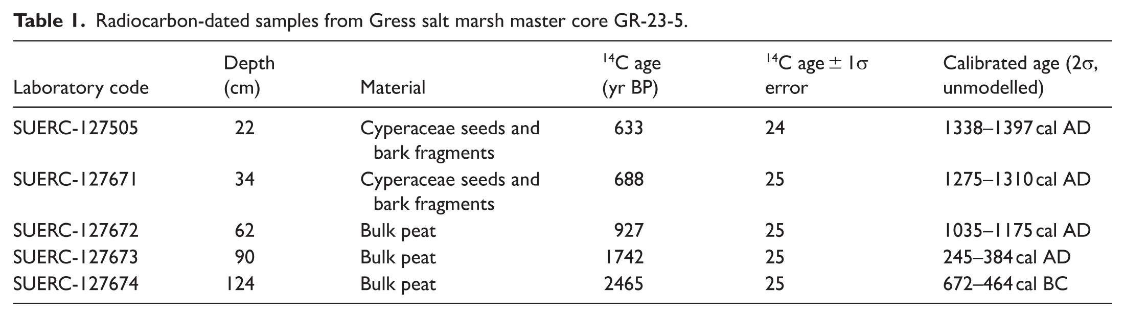
We develop a chronology using Accelerator Mass Spectrometry (AMS) ¹⁴C dates from five sediment samples. Sediments were wet sieved and placed onto a petri dish. In-situ organics such as seeds and woody (bark material) fragments (>1 cm) were carefully picked out under a binocular microscope using tweezers and placed in vials. Stems, twigs, rootlets and small wood (non-bark) fragments were avoided. There were no signs of bioturbation or sediment reworking in the sediments. All samples were cleaned with deionized water to remove sediments and other impurities, following (Kemp et al., 2013). Organics were left in a drying cabinet (c. 50°C) for several hours until all moisture is lost. For samples with insufficient macro-organics to be picked out, we prepared bulk sediment samples by obtaining only the central uncontaminated portions from the master core. Two of the five dates were based on ¹⁴C dating of plant microfossils (mostly seeds) while three were based on bulk sediment samples (Table 1). All AMS ¹⁴C dating was performed at the Scottish Universities Environmental Research Centre (SUERC) Radiocarbon Laboratory (East Kilbride, UK), following procedures described in (Dunbar et al., 2016). The five ¹⁴C radiocarbon dates (detailed in Table 1) were calibrated using the Intcal20 curve (Reimer et al., 2020) via the ‘Bchron’ package in R (Parnell and Parnell, 2016), to generate an age-depth model.

Table 1.

Radiocarbon-dated samples from Gress salt marsh master core GR-23-5.

Laboratory code	Depth (cm)	Material	¹⁴C age (yr BP)	¹⁴C age ± 1σ error	Calibrated age (2σ, unmodelled)
SUERC-127505	22	Cyperaceae seeds and bark fragments	633	24	1338–1397 cal AD
SUERC-127671	34	Cyperaceae seeds and bark fragments	688	25	1275–1310 cal AD
SUERC-127672	62	Bulk peat	927	25	1035–1175 cal AD
SUERC-127673	90	Bulk peat	1742	25	245–384 cal AD
SUERC-127674	124	Bulk peat	2465	25	672–464 cal BC

RSL reconstruction

For this study, we combined two existing UK modern diatom training datasets (Barlow et al., 2013; Kirby et al., 2023) which collectively records 594 taxa over 494 modern samples across 20 sites in UK and Ireland (Supplemental Material Figure S1) at different elevations or standardized water level index (SWLI) [equation (1)]. SWLI values is a common standardization method to account for tidal range differences between different sites in a regional training dataset for example, (Barlow et al., 2013; Gehrels, 2000; Watcham et al., 2013). At the highest elevations (SWLI > 300 or 4.21 m LOD, which is 1.43 m above the Highest Astronomical Tide at Stornoway), species such as Cavinula varistriata and Eunotia exigua dominate the assemblages. The middle elevation range between 200 (or 2.15 m LOD, which is MHWST of Stornoway) and 300 SWLI contains the most species, with Navicula cincta, Cosmioneis pusilla, Diploneis didyma dominating, alongside other Navicula species. At the lowest elevations below 200 SWLI, Achnanthes lemmermannii, Psuedostausira elliptica and Planothidium deliculatum dominate, with lower abundances of Opephora marina and Paralia sulcata.

In typical RSL reconstruction studies, a transfer function (TF) method is employed to utilize all proxy data to generate predictions for every sample in a sediment profile, based upon fit with the modern training dataset. Initially, we attempted multiple TFs for our reconstruction, but the results did not align with lithological, sedimentological and diatom biostratigraphy results. To understand why, we used the modern analogue technique (MAT) to analyse the modern diatom training dataset (Watcham et al., 2013) and concluded that all 46 fossil diatom samples in GR-23-5 were determined to have poor modern analogues in the modern training dataset (Supplemental Material Table S2).

As a result, we use a qualitative visual assessment (VA) method to reconstruct PMSEs for each sample depth of GR-23-5, consequently RSL elevations, and finally a continuous RSL reconstruction. TF approaches (Gehrels, 2000; Horton et al., 2006; Kemp et al., 2015; Zong and Horton, 1999) were explored as part of the initial analysis. However, the quantitative assessment of the fit between the modern and fossil dataset showed this was not a suitable approach in this instance, hence we utilized the VA approach advocated by Woodroffe (Woodroffe et al., 2023) and Long (Long et al., 2010, 2012) when similar issues were encountered at salt marshes in Greenland.

The VA method is more selective in the weight it places on certain taxa and considers trends in adjacent samples. Although the TF method is mathematically robust compared to the qualitative VA approach, previous studies demonstrated the potential robustness of VA as the ‘common sense, subjective’ interpretation of multi-proxy data to reconstruct PMSEs and hence RSL histories (Long et al., 2010, 2012; Woodroffe et al., 2023; Woodroffe and Long, 2009).

The VA method considers the presence of key species with narrow elevation ranges to reconstruct PMSEs, with associated errors given by the overlapping elevation ranges of these key species. Likewise, absence of such species allows us to exclude their elevation range from the reconstructed PMSEs. The structure of VA criteria in this work broadly follows similar RSL reconstruction studies (Long et al., 2010, 2012; Woodroffe et al., 2023). Only species > 5% tical in the modern training dataset and GR-23-5 were regarded as ‘present’. The VA criteria used in this work are specified in (Supplemental Material Table S1). We checked the PMSEs against other lithological data for a semi-independent check of the results.

Sample depths are first acquired by subtracting the measured surface orthographic height of the master core by the depth of each sample down the core. Instead of using MTL values (m LOD), we convert them to SWLI values following equation (1) below:

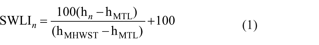
{SWLI}_{n} = \frac{100 (h_{n} - h_{MTL})}{(h_{MHWST} - h_{MTL})} + 100

(1)

where SWLI_n is the standardized water level index for sample n, h_n is the present elevation of sample n (m LOD), h_MTL is the local MTL (m LOD) and h_MHWST is the local MHWST (m LOD; Barlow et al., 2013). Reconstructions will return PMSEs in SWLI units, which will require conversion back into m LOD values. A rearrangement of equation (1) derives the following equation (2) for conversion:

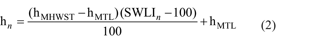
h_{n} = \frac{(h_{MHWST} - h_{MTL}) ({SWLI}_{n} - 100)}{100} + h_{MTL}

(2)

To calculate RSL elevations for each sample depth from the reconstructed PMSEs (m LOD), the PMSEs must be subtracted from $h_{n}$ to account for the sample’s depth in the sediment core (equation (3)):

R S L_{n} = h_{n} - P M S E_{n}

(3)

We applied the Error-in-Variables Integrated Gaussian Process (EIV IGP) model, using the PMSEs and geochronological data as inputs, to derive RSL trends and rates of change throughout the core’s record (Cahill et al., 2015). This Bayesian model incorporates both the temporal uncertainties from the age-depth model, and the vertical uncertainties of the reconstructed RSL elevations.

Results

We summarize our multi-proxy analysis of GR-23-5 in this section, detailing lithological (stratigraphy, grain size analysis and LOI) and biostratigraphical findings, followed by the age-depth model, reconstructed PMSEs and RSL trends and rates.

Lithology

Stratigraphy

All cores terminated in impenetrable sand or sandy peat. Above this basal unit, most cores accumulated a thick peat layer with clastic components. The peat contained clastics of mostly clay and silt in differing fractions, with no sand components. Clastics diminished towards the top of the core, transitioning to a surficial humified peat containing fibrous herbaceous roots and Sphagnum moss in some instances.

Moving seawards along the coast-perpendicular transect A–A′ (Figure 3), the elevation of the salt marsh decreased. The bottom sand layer thickened and is located at shallower depths while the peat layer thinned. Sandy deposits at the site are controlled by tides, where more sheltered inland areas only accumulated sand at lower depths in the cores. These low energy environments allowed the formation of a thicker peat layer as compared to seaward-facing regions of the marsh. Between cores 4 and 3, there was a notable rise in elevation of the basal impenetrable sand layer by 0.5 m or more. Notably, Sphagnum moss was only recorded in three of the nine cores along this transect. The core (GR-23-5) located in the middle of this transect displayed the greatest lithological variance, from silty/clayey sand to silty/clayey peat to Sphagnum moss and finally peat with herbaceous roots. Showing the greatest potential for a sea-level reconstruction, this core was selected as the master core for further analysis, and the central core for the subsequent coast-parallel transect B–B′.

Figure 3.

(a) Coast-perpendicular transect A–A′ and (b) coast-parallel transect B–B′ stratigraphy. The master core (GR 23-5) collected for analysis is highlighted in red.

Cores retrieved along the coast-parallel transect B–B′ (Figure 3) indicate that topography had little impact on the sedimentation at the field site. Most of the facies boundaries parallelled that of the topography, which implied that the sea level inundation parallel to the coast across the cores’ records was consistent, assuming similar sedimentation rates. Most cores displayed similar lithologies as the master core GR-23-5, with slightly varying thicknesses of each unit. At present day, this transect is located about 8–10 m away from the coastal boundary.

Grain size analysis

Sand and silt size fractions varied drastically with standard deviations (SDs) of 13.1 and 11.3 respectively, while the clay size fraction remained relatively consistent throughout the core with a SD of 4.41 (Figure 4). The mean percentages of sand, silt and clay are 31.8%, 61.8% and 6.45% respectively. There are multiple depths that showed a sharp decrease in sand content (102, 68, 28 cm) at 20% or more upcore, with a noticeable 50% sharp increase at 30 cm.

Figure 4.

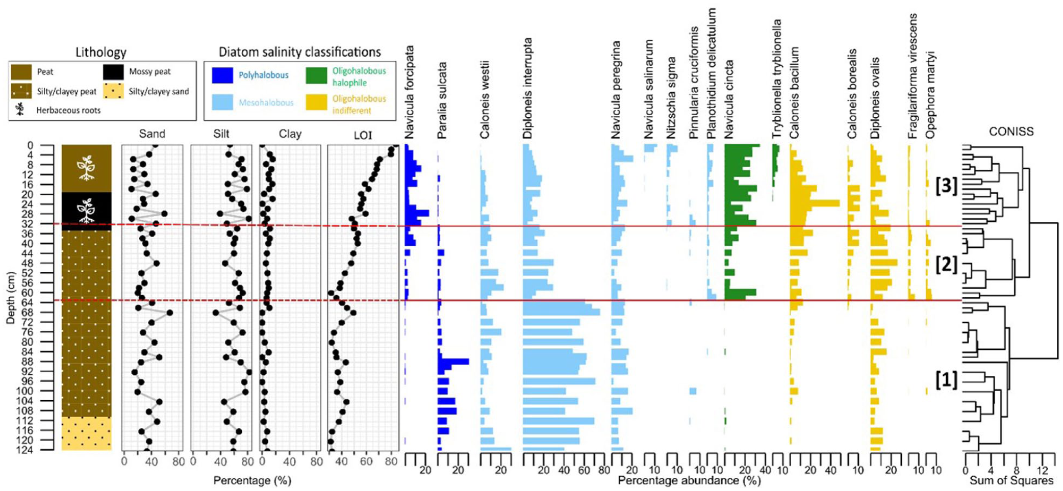
Combined plots of lithology, grain-size analysis, LOI and diatom biostratigraphy of GR-23-5. Diatom biostratigraphy only shows taxa with occurrences greater than 5% of total valves counted. Three zonations were determined using Constrained Incremental Sum of Squares (CONISS) hierarchical clustering, indicated by solid red lines, extrapolated across remaining plots as dotted red lines (Zone 1: 124–62 cm; Zone 2: 62–33 cm; Zone 3: 33–0 cm).

Loss-on-ignition (LOI)

Generally, organic content increased upcore although this pattern is interrupted at certain depths (Figure 4). Below 80 cm, RSL appears to have been fluctuating (around the intertidal range) with no clear trend, causing alternating peat and sediment accumulation. From 80 to 68 cm, peat accumulation was consistent (32–50% LOI). However, from 68 to 60 cm, LOI dropped drastically by almost 20%. Above 60 cm, there was another switch to rising organic content up to the core top.

Biostratigraphy

A total of 13,316 diatom valves from 88 species were identified in 46 samples. The 16 most common species were plotted. Constrained hierarchical clustering of a distance matrix using the CONISS algorithm (Gordon and Birks, 1972) visually contrasted the dispersion of a hierarchical classification with that derived from a broken stick model (brokenstick values which are ordered random proportions; Bennett, 1996; Legendre and Legendre, 2012) and determined three major biostratigraphic zones for GR-23-5 (Figure 4).

Zone 1 (124–62 cm) was dominated by marine polyhalobous and mesohalobous species, indicating high salinity concentrations and thus significant marine influence at time of deposition. The five main species are Paralia sulcata, Caloneis westii, Diploneis interrupta, Navicula peregrina and Diploneis ovalis. Zone 2 (62–33 cm), however, consisted of a more equal distribution of diatom species across various salinity preferences. Compared to Zone 1, there was less marine influence on the environment since the more marine polyhalobous and mesohalobous species no longer dominate. A sharp drop in Diploneis interrupta abundance (up to 50%) accompanied a sharp rise in Navicula cincta and other oligohalobous indifferent species abundances. Zone 3 (33–0 cm) presented a unique diatom assemblage. Although dominated by the less marine oligohalobous halophile and oligohalobous indifferent species (Navicula cincta, Caloneis bacillum), the more marine polyhalobous and mesohalobous species (Navicula forcipata, Diploneis interrupta and Navicula peregrina) are still of significant abundance. Compared to Zone 2, there was an observed switch to higher marine influence at the site. Although more oligohalobous indifferent species are present compared to zone 2, there was a rise in polyhalobous Navicula forcipata abundance and other salt-tolerant species are still present.

GR-23-5 presented gradual changes in diatom assemblages, except for the sharp transition between zone 1 and 2, which was not accompanied by obvious lithological changes. Generally, an upcore trend of increasing diatom taxa abundance with lower salinity preferences is observed, without transitioning to a freshwater environment. No evidence suggests disruptions to sedimentation of the marsh. In summary, GR-23-5 presents a regressive sequence, characterized by a decrease in marine influence towards the core top.

Age-depth model

Five ¹⁴C dates were used to develop a Bchron age-depth model, constraining the GR-23-5 record to 2500 years long (Figure 5). From core bottom (2440–2490 cal yr BP) up till 62 cm depth (902–952 cal yr BP), two ¹⁴C dates produced average age uncertainties of 330 years. The top half is better constrained with three ¹⁴C dates and a known coring year for the core top, with uncertainties averaging 140 years. Although three of the five ¹⁴C dates are derived from bulk peat rather than plant microfossils, we have confidence in the accuracy of the dates considering how the five dates in sequence satisfy the monotonicity constraint. Average sediment accumulation rates are modelled at ~0.04 cm yr⁻¹, with a peak of 0.23 cm yr⁻¹ (50th percentile) during 645–692 cal yr BP before dropping back to low stable rates after 500 cal yr BP (Figure 5). The peak coincides with the gradual lithological change from silty peat to Sphagnum moss at 33 cm depth (563–613 cal yr BP).

Figure 5.

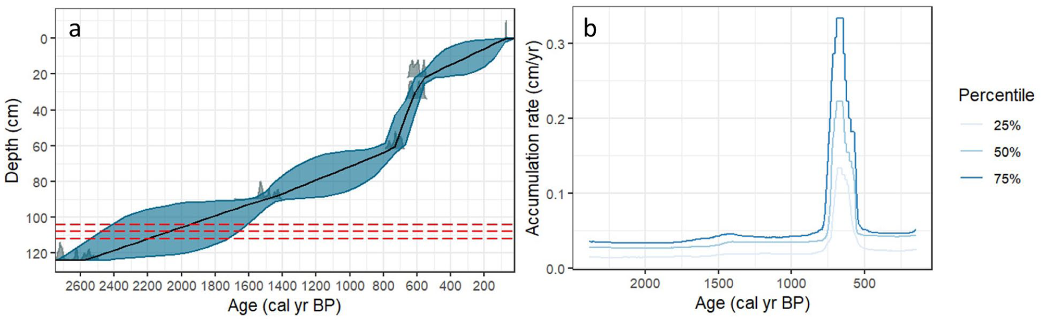
(a) Bchron age-depth model of GR-23-5, alongside the (b) Bchron-modelled accumulation rates of GR-23-5 based on five 14C radiocarbon dates (detailed in Table 1). Ages were calibrated using Intcal20 (Reimer et al., 2020). Dashed red lines indicate the three depths where maximum variance in the model were observed.

PMSE and RSL reconstructions

The lithology of GR-23-5 provides a broad idea of changes in paleo RSL at this site. Starting with the silty/clayey sand unit and an absence of organic material, the paleoenvironment was likely an intertidal flat, with the highest tides submerging the flat and lowest tides exposing it. As sea level fell, the tidal flat transitioned into a salt marsh, with vegetation first growing at the site. Over time, the incomplete decomposition of plant remains growing in acidic, waterlogged conditions started to form a peat layer. This first half of the core’s record was accompanied by a dominance of Diploneis Interrupta which is a brackish aerophilous taxa (Espinosa et al., 2006; Espinosa and Isla, 2015), known to live in supratidal environments like tidal levees or levee marshes (Vos, 1988). Continued sea level fall or stability then likely resulted in a high marsh environment or raised bog (Shennan et al., 2000), which promoted the growth of Sphagnum moss. Being a freshwater species, Sphagnum moss is a natural indicator of a high marsh environment due to its low salt tolerance (Whittle and Gallego-Sala, 2016) and is rarely found in saline habitats (Kay, 2019). This switch was accompanied by the change between biostratigraphic zone 1 and 2, where Diploneis Interrupta stopped dominating and other oligohalobous indifferent species appeared. The uppermost peat layer above the Sphagnum moss indicates a change in RSL tendency, from negative to positive, as the Sphagnum moss layer disappeared and the high marsh environment transitioned to the current low-mid marsh environment. Diatom assemblages in zone 3 also show this change, with dominance by dominated by the less marine oligohalobous halophile and oligohalobous indifferent species. Preliminarily, we can deduce that RSL has been consistently falling from the bottom of the sand layer and probably stabilized until the top of the Sphagnum moss layer, before transitioning to a RSL rise. We present further quantitative evidence below to support or reject this hypothesis.

Diploneis interrupta is the dominant species in GR-23-5, but in the modern dataset, this species only presents as >10% in 3 of the 494 samples. Diploneis interrupta is a heavily silicified diatom species that is tolerant to highly dynamic conditions with sediment suspension, tidal action and wind stress. It was likely better preserved than other species post-deposition, resulting in overrepresentation. Similar findings were reported by other studies with overrepresented, heavily silicified diatom species (Kirby et al., 2023; Watermann et al., 2004), including the geographically proximal RSL reconstruction by (Jordan et al., 2010). Performing the MAT analysis after removing this species showed higher minDC values for the fossil samples as compared to before, with still 0 ‘good’ or ‘close’ modern analogues. Removing this dominant species artificially increases the other species’ abundance linearly, which is an inaccurate representation of the paleoenvironment. Hence, Diploneis interrupta counts were retained for reconstructions.

To try and improve the modern training set we also collected 15 modern samples at Gress, across an elevation range of 1.45 m LOD to 2.61 m LOD from varied environments. However, less than half the samples have sufficiently well-preserved diatom valves for counting. Of the five modern samples that have been counted, none of them resemble the diatom assemblage for zone 1 of GR-23-5 with a dominance of Diploneis interrupta. All the samples have Diploneis interrupta as <10% abundance. Considering the lack of data, we did not include the Gress modern diatom assemblage data into this study.

To reconstruct the PMSEs of the uppermost few samples of the core, we used key species with narrow elevation ranges such as Nitzschia sigma and Tryblionella tryblionella to reconstruct the PMSEs. For the bottom half of the core, due to the dominance of Diploneis interrupta, we could only use species like Caloneis westii and Diploneis ovalis to constraint the PMSEs, which have wider elevation ranges. Considering the dominance of Diploneis interrupta, we decided not to use the absence of any key species as part of the VA criteria, unlike other published work with no overdominance of a certain species (Long et al., 2010, 2012; Woodroffe et al., 2023). Doing so may also reduce the uncertainty of reconstructed PMSEs biasedly in this case. The resulting PMSEs for each sample are given in Supplemental Material Table S1, with a justification.

Combining the reconstructed PMSEs (Supplemental Material Table S1) and the age-depth model, we used an EIV IGP model (Cahill et al., 2015) to produce an RSL reconstruction (Figure 6). The PMSEs (Figure 6a) showed a generally consistent marsh elevation throughout the core’s record, with vertical uncertainties ranging from 0.7 to 1 m (2σ), meaning that the elevation of the marsh surface is a consequence of the rate of sediment accumulation.

Figure 6.

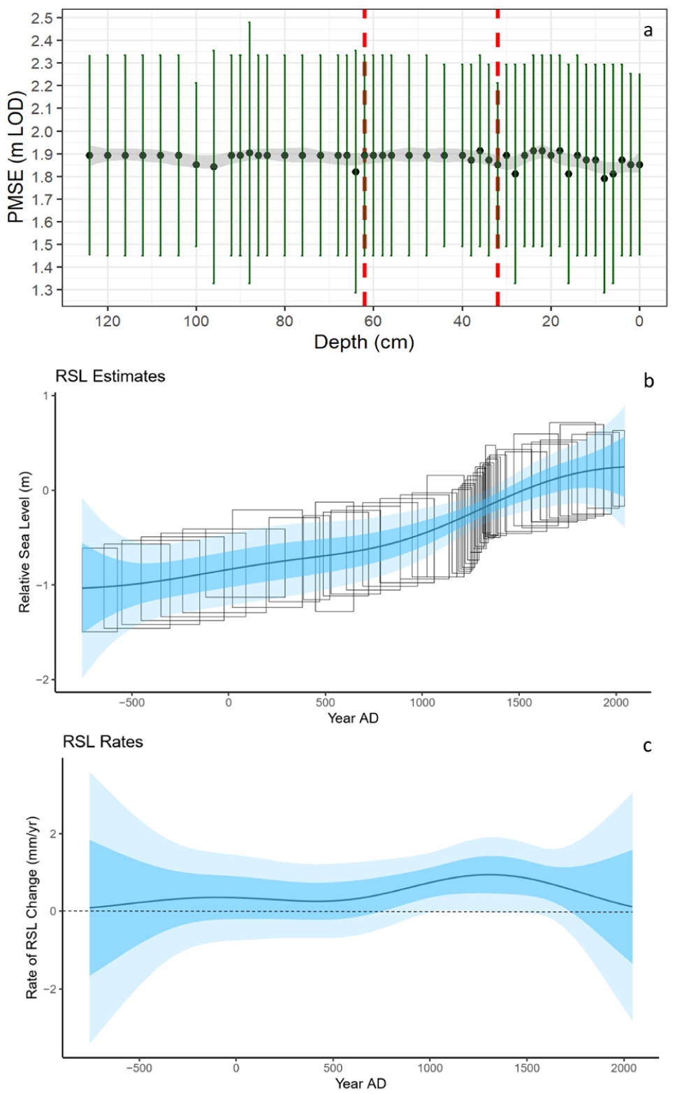
(a) Paleomarsh surface elevation (PMSE) calculated for GR-23-5 based on visual assessment method through the fossil core. Dotted red lines indicate the zonation boundaries determined by CONISS based on diatom biostratigraphy shown in Figure 4. (b) Reconstructed RSL reconstruction and (c) rate RSL change (dotted line showing zero rate of RSL change), both modelled using an Errors-in-Variables Integrated Gaussian Process (EIV IGP) model (Cahill et al., 2015).

Discussion

Reconstructing past sea level in the absence of modern analogues

Our reconstruction of paleo RSL shows a ~1.2 ± 1 m (2σ) rise throughout the core’s 2500-year record (Figure 6b). Maximum vertical uncertainties of RSL values range from 0.7 to 1 m (2σ) while temporal uncertainties range from less than 50 years near the dated horizons, to a maximum of 400 years. Notably, the rate of RSL peaked at c. AD 1300, corresponding to the lithological and biostratigraphical change at 33 cm depth. Modelled rates of RSL change do not exceed 1.5 mm yr⁻¹ (Figure 6c).

Our reconstruction holds value as the first continuous RSL record for the Late-Holocene outside of mainland Scotland. We acknowledge that the lack of a local modern training dataset, when the existing regional dataset is proven to be a misfit for the fossil diatoms in GR-23-5 is a limitation of this work. Future work to build a substantial local modern training dataset from Gress and its surrounding locations (Outer Hebrides) will help us better understand the diatom species distribution in the region. In any case, we substantiate our VA method to reconstruct PMSEs with complementary proxies in this work to produce a reliable sea level reconstruction, by only considering the presence of key species at >5% abundance threshold.

Vertical RSL errors in this study are contributed by several factors. GPS levelling error in the field amounts to ~0.01 m. Human errors when subsampling the core into 1 cm slices were minimized by using thin surgical blades, and we accounted for an error of 0.1 cm. Majority of the vertical uncertainty results from the VA reconstruction due to the ~50 SWLI elevation range of diatom taxa used in the VA criteria. This translates to a vertical precision of around ±0.45 m for every reconstructed PMSE. In previous studies, the errors derived from VA-derived PMSEs were not specifically defined in statistical terms. In our study, we define our vertical reconstruction errors of around ± 0.45 m to be conservatively of ±1σ error, making it comparable with TF-derived RSL studies. The final vertical RSL errors (±1σ) were calculated as a root squared error arising from the VA reconstruction, GPS levelling and human error during subsampling.

Changes in tidal range over time constitute another source of uncertainty in RSL reconstructions (Gehrels, 2000; Kirby et al., 2023; Shennan and Horton, 2002). Since RSL reconstructions rely on knowing the height of MHWST above MTL, an unrecognized increase in this range over time could be misinterpreted as a RSL rise, and vice versa (Kirby et al., 2023). Based on modelling results using 37 years of hourly Stornoway tide gauge data (1976–2013), we determine that the estimated annual change in spring tidal range is −0.0031 m yr⁻¹, amounting to a cumulative −0.11 m over the length of the available data (Supplemental Material Figure S2). Unfortunately, we cannot extrapolate the spring tidal range change over our 2500-year record. Nonetheless, the spring tidal range has been decreasing over the tide gauge’s record and if anything, will reflect as an artefact of a RSL fall in our reconstruction, which was not observed. We also note that the mesotidal environment at Gress necessitates the lower resolution of RSL reconstruction compared to other sites with a smaller tidal range. The marsh accumulation at Gress is also very low at ~0.04 cm yr⁻¹, for majority of the record, limiting the resolution of the fossil diatom biostratigraphy data. Our vertical reconstruction errors sit at 16% of the mean tidal range at Gress.

Late-Holocene RSL at Gress

From an assessment of the sedimentology, biostratigraphy and chronology, considering the uncertainty discussed, we postulate that the Gress salt marsh has experienced a rising RSL over the last 2500 years, associated with a general pattern of marsh progradation under low rates of RSL rise and a low, sustained sediment supply (Figure 6). This is presumed to keep up with the sea level rise at Gress, considering the LOI trend upcore. A closer inspection of the biostratigraphy data and LOI trend suggests a change from a negative to a positive local sea-level tendency at the transition between zones 1 and 2 of the biostratigraphy, corresponding to the ~20% decrease in LOI across depths 68–60 cm (Figure 4). We highlight the sharp drop in abundance of Diploneis interrupta (up to ~50%), alongside the appearance of Navicula cincta and other less-salinity-tolerant oligohalobous–halophilous and oligohalobous-indifferent species, suggesting a change in environment at this time. This change in biostratigraphy and LOI was not observed in the lithology. However, the final RSL reconstruction does show an increase in RSL rate from c. AD 900–AD 1300, largely corresponding to this major biostratigraphic and LOI change. We initially suspected the peak in accumulation rate at c. 900 cal yr BP was due to two ¹⁴C dates being close in ages–34 cm (563–613 cal yr BP) and 22 cm (609–657 cal yr BP) depths. It could be attributed to sampling issue or rapid sedimentation. By running two additional Bchron models with four ¹⁴C dates, excluding the 34 cm depth and 22 cm depth dates respectively, we observed a peak of similar age and magnitude in each. This gives us confidence that the peak is reliable and representative of a physical environmental change that caused rapid marsh sedimentation at Gress, rather than an artefact of the model.

Organic-rich, low-density salt-marsh sediments exhibit susceptibility to compaction mechanisms that induce post-depositional deformation within stratigraphic sequences utilized for RSL reconstructions (Brain et al., 2017). Within low-energy intertidal settings, such compaction drives vertical settlement and subsidence of depositional surfaces relative to the tidal frame, mimicking local-scale relative sea-level rise (Brain, 2016; Brain et al., 2012). This process introduces inaccuracies into estimates of both the magnitude and rate of past sea-level fluctuations derived from salt-marsh archives (Brain, 2015; Kaye and Barghoorn, 1964). Nevertheless, research demonstrates that salt-marsh sequences characterized by homogeneous lithology or comprising shallow, near-surface deposits within regressive stratigraphic successions exhibit minimal compaction effects (Brain et al., 2012). Empirical analyses and modelling further establish that compaction-driven depression of sea-level indicators correlates positively with the thickness of overlying sedimentary units and the cumulative depth of the sediment column (Brain, 2016; Brain et al., 2017). Given the relatively short length of GR-23-5 and multi-proxy evidence supporting RSL rise at Gress over the past 2500 years, sediment compaction is recognized as a source of uncertainty but remains uncorrected in this RSL reconstruction owing to its inferred insubstantial influence.

Late-Holocene RSL changes across northwest Scotland

Here, we discuss the interplay of factors driving RSL change at Gress – GIA, barystatic sea level change, local influence and marsh sedimentation rate. Over the 2500-year record, our results show that Gress RSL rates vary from 0 to 0.9 mm yr⁻¹. The GIA-driven local RSL rise signal of Gress at present day, however, is only modelled to 0.1–0.2 mm yr⁻¹ (Bradley et al., 2023). The ‘background’ marsh sedimentation rate largely remained at 0.4 mm yr⁻¹, with a peak of 2.3 mm yr⁻¹ from AD 950 to AD 1300. Synthesizing the above, we can deduce that the combined effects of both attribute to be at most 0.6 mm yr⁻¹ of RSL rise, largely fitting our reconstruction. In extreme cases of more than 0.6 mm yr⁻¹ RSL rise at Gress, there is a possible 0.3 mm yr⁻¹ of unexplained RSL rise. This difference can be attributed to barystatic sea level change, thermal influence on ocean waters, geoid changes or local factors, which are difficult to untangle. Nonetheless, we can still conclude the marsh surface elevation continued to keep pace with background GIA, either by stable or increased barystatic sea level rise, albeit at a slower rate.

We compare our reconstruction to the only other Holocene reconstruction from the Outer Hebrides, in Harris (Jordan et al., 2010), and the only other two Late-Holocene salt marsh reconstructions in northwest Scotland (Barlow et al., 2014). Jordan et al. (2010) suggested a rapid Mid-Holocene RSL rise ~6200 BP, followed by fluctuations until stabilization after ~3100–2100 BP. This is generally in line with the two other Late-Holocene records by Barlow et al. (2014), which can be summarized to show a generally stable RSL trend for the last 1500–2500 years (Figure 7). However, Barlow et al. (2014) noted that the records from Loch Laxford and Kyle of Tongue show a consistent increase in RSL c. AD 1945–1980. Our Gress reconstruction similarly suggests an overall RSL rise over the last 2500 years, with an accelerated increase in RSL peaking at c. AD 1300, which aligns with the idea of accelerated eustatic rise at Gress or Outer Hebrides. Apparent temporal discrepancies between our reconstructed sea-level trends from Gress and those documented by Barlow et al. (2014) could arise from differential geomorphic responses across sites.

Figure 7.

Late-Holocene continuous salt-marsh reconstructions from Scotland plotted with 2σ age and reconstructed RSL errors. RSL records of Loch Laxford and Kyle of Tongue are plotted with results from LA-3, LA-6 and KT 3 in Barlow et al. (2014).

Our results help validate the regional GIA model that depict Gress as a proximal location to a RSL zero isobase (Bradley et al., 2023), with minimal deviation from barystatic trends. Critically, our work supports the modelled RSL zero isobase contour positions, with Gress lying just outside the RSL zero isobase contour and hence experiencing a 0.1–0.2 mm yr⁻¹ GIA-driven present-day local RSL rise signal (Bradley et al., 2023). Loch Laxford and Kyle of Tongue, both lie on or just outside the modelled RSL zero isobase contour, experience a 0–0.1 mm yr⁻¹ GIA-driven present-day local RSL rise signal (Barlow et al., 2014; Bradley et al., 2023). GIA modelling results (Bradley et al., 2023) are supported by our Gress reconstruction which shows a more pronounced rising sea level trend at a location less affected by GIA land uplift than Loch Laxford and Kyle of Tongue. However, we would like to highlight two caveats. First, as noted in Bradley et al. (2023), the GIA models do not consider 20th century sea level acceleration. Second, Gress and Barlow et al. (2014)’s study sites are all close to the border of the modelled RSL zero isobase contour, which shifts with different model input parameters. This study, alongside comparisons with Barlow et al. (2014) RSL records and Bradley et al. (2023) GIA models, highlight the intricacies of multiple driving factors on Late-Holocene RSL trends in northwest Scotland.

We evaluate whether there are signs of RSL rise during the last two millennia in the uplifting coastlines of northwest Scotland, by analysing existing tide gauge data in northwest Scotland. Linear trends of MSL rise since the 19th century were recorded as 0.76 ± 0.28 and 0.94 ± 0.07 mm yr⁻¹ at Wick and Aberdeen respectively (Woodworth et al., 2009). Tide gauge measurements over a fortnight in 1859 at Wick and Thurso were processed, giving MSL rises of 3.728 ± 0.578 and 1.681 ± 0.552 mm yr⁻¹ (Woodworth, 2017). We also analysed 48 years of monthly MSL data from Stornoway tide gauge (PSMSL, 2025), closest to Gress, and modelled present-day MSL to rise at 3.45 mm yr⁻¹ (Supplemental Material Figure S3). This is consistent with our Gress reconstruction, though mindful of the large vertical uncertainties. Despite the magnitude differences in rate of RSL rise, all sources support the hypothesis of 20th century sea-level acceleration in northwest Scotland, surpassing the rate of background RSL decline (minimum of c. −0.4 mm yr⁻¹).

RSL trends from northwest Scotland cannot be uniformly interpreted through a single locality’s data alone. While our Late-Holocene salt-marsh reconstruction broadly aligns with other regional records, some intricate variations persist. These variations reflect the spatiotemporal dynamics of sea-level change driven by the BIIS’ glaciation history and interactions among atmospheric, oceanic, and cryospheric systems operating across differing scales (Gehrels, 2010; Long et al., 2015; Smith et al., 2019). Such complexity precludes simplistic aggregation of records into a unified regional narrative. There is sparse availability of high-resolution Late-Holocene RSL reconstructions in the region. Given the spatially heterogeneous responses to complex processes in a data-sparse region, we cannot decipher if sea-level change in northwest Scotland is mostly controlled by global, regional or local processes.

Conclusion

Salt-marsh sediments can provide precise and near-continuous, high-resolution reconstructions of Late-Holocene RSL (Brain et al., 2017). Using a multi-proxy (lithology, sedimentology, biostratigraphy, chronology) approach, we produce a high-resolution Late-Holocene RSL record at Gress in northwest Scotland, using salt marsh sediments. The modelled results show a largely rising RSL at Gress over the last 2500 years, with an accelerated RSL rise from c. AD 950–AD 1300. This study presents evidence that local RSL rise at Gress likely exceeded 0.2 mm yr^-1 (the modelled background rate of Late-Holocene RSL fall in northwest Scotland) from 500 BCE to AD 2022, especially at c. AD 1300. We cannot reject the hypothesis of sea level acceleration during the last two millennia, but such a signal, if present, is not significantly recorded in salt marsh sediments in the region. Comparing our record to proximal existing Late-Holocene reconstructions (Barlow et al., 2014) emphasizes the spatial and temporal complexity of RSL change in the region. We also evaluate the results of existing reconstructions in the context of the recently modelled RSL zero isobase contour (Bradley et al., 2023), and discuss the implications of such RSL records in future GIA modelling work. To reconcile spatially variable sea-level change patterns, it is essential to incorporate considerations of how sediment accumulation dynamics, tidal inundation thresholds and organic productivity within salt marshes modulate their sensitivity to RSL fluctuations over time. Investigating the controls on Late-Holocene RSL changes requires a broader spatial distribution and greater temporal continuity of precise RSL reconstructions across northwest Scotland.

Supplemental Material

sj-docx-1-hol-10.1177_09596836261450835 – Supplemental material for A 2500-year record of relative sea-level change at Gress, Isle of Lewis, northwest Scotland using salt marsh sediments

Supplemental material, sj-docx-1-hol-10.1177_09596836261450835 for A 2500-year record of relative sea-level change at Gress, Isle of Lewis, northwest Scotland using salt marsh sediments by Khai Ken Leoh, Natasha L. M. Barlow, Sue Dawson, Uisdean Nicholson and Adam D. Switzer in The Holocene

Footnotes

Acknowledgements

The authors thank Weilun Qin from TU Delft for his contributions during fieldwork.

ORCID iDs

Khai Ken Leoh

Natasha L. M. Barlow

Sue Dawson

Uisdean Nicholson

Adam D. Switzer

Author contribution(s)

Khai Ken Leoh: Data curation; Formal analysis; Funding acquisition; Investigation; Methodology; Writing – original draft; Writing – review & editing.

Natasha L. M. Barlow: Conceptualization; Funding acquisition; Investigation; Methodology; Project administration; Resources; Supervision; Validation; Writing – review & editing.

Sue Dawson: Conceptualization; Investigation; Resources; Supervision; Writing – review & editing.

Uisdean Nicholson: Conceptualization; Funding acquisition; Investigation; Project administration; Resources; Validation; Writing – review & editing.

Adam D. Switzer: Conceptualization; Supervision; Writing – review & editing.

Funding

The authors disclosed receipt of the following financial support for the research, authorship, and/or publication of this article: This work was primarily supported by the Nanyang Technological University’s CN Yang Scholars Programme (Nanyang Scholarship), awarded to K.K.L. A.D.S and K.K.L are supported by Singapore Ministry of Education Academic Research Fund grants MOE2019-T3-1-004 and RG158/24. U.N, Natasha L.M.B and S.D were partly funded by NERC through the Discipline Hopping for Environmental Solutions Fund.

Declaration of conflicting interests

The authors declared no potential conflicts of interest with respect to the research, authorship, and/or publication of this article.

Supplemental material

Supplemental material for this article is available online.

References

Barlow

NLM

Long

Saher

, et al. (2014) Salt-marsh reconstructions of relative sea-level change in the North Atlantic during the last 2000 years. Quaternary Science Reviews 99: 1–16.

Barlow

NLM

Shennan

Long

, et al. (2013) Salt marshes as late Holocene tide gauges. Global and Planetary Change 106: 90–110.

Bennett

(1996) Determination of the number of zones in a biostratigraphical sequence. New Phytologist 132: 155–170.

Bradley

Ely

Clark

, et al. (2023) Reconstruction of the palaeo-sea level of Britain and Ireland arising from empirical constraints of ice extent: Implications for regional sea level forecasts and North American ice sheet volume. Journal of Quaternary Science 38: 791–805.

Bradley

Milne

Shennan

, et al. (2011) An improved glacial isostatic adjustment model for the British Isles. Journal of Quaternary Science 26: 541–552.

Brain

(2015) Compaction. In: Shennan

Long

Horton

(eds) Handbook of Sea-Level Research. John Wiley & Sons, pp.452–469.

Brain

(2016) Past, present and future perspectives of sediment compaction as a driver of relative sea level and coastal change. Current Climate Change Reports 2: 75–85.

Brain

Kemp

Hawkes

, et al. (2017) Exploring mechanisms of compaction in salt-marsh sediments using common era relative sea-level reconstructions. Quaternary Science Reviews 167: 96–111.

Brain

Long

Woodroffe

, et al. (2012) Modelling the effects of sediment compaction on salt marsh reconstructions of recent sea-level rise. Earth and Planetary Science Letters 345-348: 180–193.

10.

Cahill

Kemp

Horton

, et al. (2015) Modeling sea-level change using errors-in-variables integrated Gaussian processes. Annals of Applied Statistics 9: 547-571.

11.

Clark

Ely

Fabel

, et al. (2022) BRITICECHRONO maps and GIS data of the last British-Irish Ice Sheet 31 to 15 ka, including model reconstruction, geochronometric age spreadsheet, palaeotopographies and coastline positions. Pangaea. Pangaea.

12.

Clark

Farrell

Peltier

(1978) Global changes in postglacial sea level: A numerical calculation. Quaternary Research 9: 265–287.

13.

Cleve-Euler

(1952) Die Diatomeen von Schweden und Finland. Kungliga Svenska Vetenskaps Akademiens Handlinger Ser. 4 3: 1–153.

14.

Davey

(2025) Historical maps–landmark information group. Available at: https://www.landmark.co.uk/products/historical-maps/ (accessed 12 March 2026).

15.

Denys

(1991) A Check-List of the Diatoms in the Holocene Deposits of the Western Belgian Coastal Plain with a Survey of Their Apparent Ecological Requirements. Ministerie van Economische Zaken Belgium.

16.

Dunbar

Cook

Naysmith

, et al. (2016) AMS 14C dating at the Scottish Universities Environmental Research Centre (SUERC) radiocarbon dating laboratory. Radiocarbon 58: 9–23.

17.

Dutton

Carlson

Long

, et al. (2015) Sea-level rise due to polar ice-sheet mass loss during past warm periods. Science 349: aaa4019.

18.

Dutton

Lambeck

(2012) Ice volume and sea level during the last interglacial. Science 337: 216–219.

19.

Edwards

(2006) Mid-to late-Holocene relative sea-level change in southwest Britain and the influence of sediment compaction. Holocene 16: 575–587.

20.

Espinosa

Hassan

Isla

(2006) Diatom distribution across a temperate microtidal marsh, Mar Chiquita coastal lagoon, Argentina. Thalassas An International Journal of Marine Sciences 22: 9–16.

21.

Espinosa

Isla

(2015) Modern diatom assemblages in surface sediments from meso-macrotidal estuaries of Patagonia, Argentina. Pan-American Journal of Aquatic Sciences 10: 29-43.

22.

Gehrels

(2000) Using foraminiferal transfer functions to produce high-resolution sea-level records from salt-marsh deposits, Maine, USA. Holocene 10: 367–376.

23.

Gehrels

(2010) Late Holocene land- and sea-level changes in the British Isles: Implications for future sea-level predictions. Quaternary Science Reviews 29: 1648–1660.

24.

Goelzer

Nowicki

Payne

, et al. (2020) The future sea-level contribution of the Greenland ice sheet: A multi-model ensemble study of ISMIP6. Cryosphere 14: 3071–3096.

25.

Gordon

Birks

HJB

(1972) Numerical Methods in Quaternary palaeoecology I. Zonation of pollen diagrams. New Phytologist 71: 961–979.

26.

Gregory

Griffies

Hughes

, et al. (2019) Concepts and terminology for sea level: Mean, variability and change, both local and global. Surveys in Geophysics 40: 1251–1289.

27.

Haggart

(2008) Relative sea-level change in the Beauly Firth, Scotland. Boreas 15: 191-207.

28.

Hamilton

Lloyd

Barlow

NLM

, et al. (2015) Late glacial to holocene relative sea-level change in Assynt, northwest Scotland, UK. Quaternary Research 84: 214–222.

29.

Hartley

Barber

Carter

, et al. (1996) An Atlas of British Diatoms. Biopress.

30.

Hartley

Ross

Williams

(1986) A check-list of the freshwater, brackish and marine diatoms of the British Isles and adjoining coastal waters. Journal of the Marine Biological Association of the United Kingdom 66: 531–610.

31.

Hassan

Espinosa

Isla

(2006) Modern diatom assemblages in surface sediments from estuarine systemsin the Southeastern Buenos Aires Province, Argentina. Journal of Paleolimnology 35: 39-53.

32.

Heiri

Lotter

Lemcke

(2001) Loss on ignition as a method for estimating organic and carbonate content in sediments: Reproducibility and comparability of results. Journal of Paleolimnology 25: 101–110.

33.

Hendey

(1964) An Introductory Account of the Smaller Algae of British Coastal Waters: Part V, Bacillariophyceae [Diatoms]. Otto Koeltz Science Publishers.

34.

Holgate

Matthews

Woodworth

(2012) New data systems and products at the permanent service for mean sea level. Journal of Coastal Research 29: 493–504.

35.

Horton

Corbett

Culver

, et al. (2006) Modern saltmarsh diatom distributions of the Outer Banks, North Carolina, and the development of a transfer function for high resolution reconstructions of sea level. Estuarine Coastal and Shelf Science 69: 381–394.

36.

Horton

Zong

Hillier

, et al. (2007) Diatoms from Indonesian mangroves and their suitability as sea-level indicators for tropical environments. Marine Micropaleontology 63: 155-168.

37.

Horwath

Gutknecht

Cazenave

, et al. (2022) Global sea-level budget and ocean-mass budget, with a focus on advanced data products and uncertainty characterisation. Earth System Science Data 14: 411–447.

38.

Jordan

Smith

Dawson

, et al. (2010) Holocene relative sea-level changes in Harris, Outer Hebrides, Scotland, UK. Journal of Quaternary Science 25: 115–134.

39.

Juggins

(2015) Rioja: Analysis of quaternary science data. Available at: https://cran.r-project.org/web/packages/rioja/index.html (accessed 6 May 2015).

40.

Juggins

(2019) Package ‘rioja’. RCRAN.

41.

Kaye

Barghoorn

(1964) Late Quaternary sea-level change and crustal rise at Boston, Massachusetts, with notes on the autocompaction of peat. Geological Society of America Bulletin 75: 63–80.

42.

Kay

(2019) Impacts of Warming, Drought and Sea Level Rise on Ombrotrophic Peatlands. Manchester Metropolitan University.

43.

Kemp

Horton

Engelhart

(2013) Late quaternary relative sea-level changes at mid-latitudes. Encyclopedia of Quaternary Science 9: 489–494.

44.

Kemp

Telford

Shennan

(2015) Transfer Functions, Handbook of Sea-Level Research. John Wiley and Sons, pp.470–499.

45.

Kershaw

(1997) A modification of the Troels-Smith system of sediment description and portrayal. Quaternary Australasia 15: 63–68.

46.

Khan

Ashe

Shaw

, et al. (2015) Holocene relative sea-level changes from near-, intermediate-, and far-field locations. Current Climate Change Reports 1: 247–262.

47.

Kirby

Garrett

Gehrels

(2023) Holocene relative sea-level changes in northwest Ireland: An empirical test for glacial isostatic adjustment models. Holocene 33: 926–938.

48.

Kopp

Simons

Mitrovica

, et al. (2009) Probabilistic assessment of sea level during the last interglacial stage. Nature 462: 863–867.

49.

Lecavalier

Milne

Simpson

MJR

, et al. (2014) A model of Greenland ice sheet deglaciation constrained by observations of relative sea level and ice extent. Quaternary Science Reviews 102: 54–84.

50.

Legendre

(2012) Numerical Ecology. Elsevier.

51.

Hai

, et al. (2024) Reconciled estimation of Antarctic ice sheet mass balance and contribution to global sea level change from 1996 to 2021. Science China Earth Sciences 67: 3562–3578.

52.

Lloyd

Zong

Fish

, et al. (2013) Holocene and Lateglacial relative sea-level change in north-west England: Implications for glacial isostatic adjustment models. Journal of Quaternary Science 28: 59–70.

53.

Long

Barlow

NLM

Busschers

, et al. (2015) Near-field sea-level variability in northwest Europe and ice sheet stability during the last interglacial. Quaternary Science Reviews 126: 26–40.

54.

Long

Woodroffe

Milne

, et al. (2010) Relative sea level change in west Greenland during the last millennium. Quaternary Science Reviews 29: 367–383.

55.

Long

Woodroffe

Milne

, et al. (2012) Relative sea-level change in Greenland during the last 700 yrs and ice sheet response to the Little Ice Age. Earth and Planetary Science Letters 315-316: 76–85.

56.

Milne

Shennan

(2013) Isostasy: Glaciation-induced sea-level change. Encyclopedia of Quaternary Science 9: 452–459.

57.

Mitrovica

Gomez

Morrow

, et al. (2011) On the robustness of predictions of sea level fingerprints. Geophysical Journal International 187: 729–742.

58.

Parnell

(2016) Package ‘Bchron’. Citeseer.

59.

Patton

Hubbard

Bradwell

, et al. (2013) Rapid marine deglaciation: Asynchronous retreat dynamics between the Irish Sea Ice Stream and terrestrial outlet glaciers. Earth Surface Dynamics 1: 53–65.

60.

PSMSL (2025) Tide gauge data: Station 314. Available at: https://psmsl.org/data/obtaining/stations/314.php (accessed 24 April 2025).

61.

Purkey

Johnson

Chambers

(2014) Relative contributions of ocean mass and deep steric changes to sea level rise between 1993 and 2013. Journal of Geophysical Research Oceans 119: 7509–7522.

62.

Reimer

Austin

Bard

, et al. (2020) The IntCal20 Northern Hemisphere radiocarbon age calibration curve (0–55 cal kBP). Radiocarbon 62: 725-757.

63.

Ross and Cromarty (1898) Isle of Lewis Sheet XV. Ordnance Survey. Six-inch to the Mile. National Library of Scotland.

64.

Ross-shire (1852) Island of Lewis, Sheet 15. Ordnance Survey. Six-inch to the Mile.: National Library of Scotland.

65.

Round

Crawford

Mann

(1990) Diatoms: biology and morphology of the genera. Cambridge University Press.

66.

Schumacher

King

Rougier

, et al. (2018) A new global GPS data set for testing and improving modelled GIA uplift rates. Geophysical Journal International 214: 2164–2176.

67.

Scourse

Ward

Wainwright

, et al. (2024) An interactive visualization and data portal tool (PALTIDE) for relative sea level and palaeotidal simulations of the northwest European shelf seas since the Last Glacial Maximum. Journal of Quaternary Science 39: 831-838.

68.

Shennan

Bradley

Edwards

(2018) Relative sea-level changes and crustal movements in Britain and Ireland since the Last Glacial Maximum. Quaternary Science Reviews 188: 143–159.

69.

Shennan

Horton

(2002) Holocene land- and sea-level changes in Great Britain. Journal of Quaternary Science 17: 511–526.

70.

Shennan

Lambeck

Horton

, et al. (2000) Late Devensian and Holocene records of relative sea-level changes in northwest Scotland and their implications for glacio-hydro-isostatic modelling. Quaternary Science Reviews 19: 1103–1135.

71.

Shennan

Milne

Bradley

(2012) Late Holocene vertical land motion and relative sea-level changes: Lessons from the British Isles. Journal of Quaternary Science 27: 64–70.

72.

Smith

Barlow

NLM

Bradley

, et al. (2019) Quaternary sea level change in Scotland. Earth and Environmental Science Transactions of the Royal Society of Edinburgh 110: 219–256.

73.

Smith

Cullingford

Firth

(2000) Patterns of isostatic land uplift during the Holocene: Evidence from mainland Scotland. Holocene 10: 489–501.

74.

Switzer

Pile

(2015) Grain size analysis. In: Shennan

Long

Horton

(eds) Handbook of Sea-level Research. John Wiley & Sons, pp.331–346.

75.

Troels-Smith

(1955) Karakterisering af løse jordarter. Danmarks Geologiske Undersøgelse IV. Række 3: 1–73.

76.

UHSLC (2017) UHSLC stations. Available at: https://uhslc.soest.hawaii.edu/stations/?stn=295#datums (accessed 24 April 2025).

77.

Vos

(1988) Methodological aspects of paleo-ecological diatom research in coastal areas of the Netherlands. Geologie en Mijnbouw 67: 31–40.

78.

Vos

De Wolf

(1993) Diatoms as a tool for reconstructing sedimentary environments in coastal wetlands; methodological aspects. Hydrobiologia 269-270: 285–296.

79.

Ward

Neill

Scourse

, et al. (2016) Sensitivity of palaeotidal models of the northwest European shelf seas to glacial isostatic adjustment since the Last Glacial Maximum. Quaternary Science Reviews 151: 198-211.

80.

Watcham

Shennan

Barlow

NLM

(2013) Scale considerations in using diatoms as indicators of sea-level change: Lessons from Alaska. Journal of Quaternary Science 28: 165–179.

81.

Watermann

Freund

Gerdes

(2004) Distribution and palaeoecological indicator value of diatoms in Holocene coastal deposits of the southern North Sea (Lower Saxony, Germany). E&G Quaternary Science Journal 54: 48–70.

82.

Whittle

Gallego-Sala

(2016) Vulnerability of the peatland carbon sink to sea-level rise. Scientific Reports 6: 28758.

83.

Woodroffe

Long

(2009) Salt marshes as archives of recent relative sea level change in West Greenland. Quaternary Science Reviews 28: 1750–1761.

84.

Woodroffe

Wake

Kjeldsen

, et al. (2023) Missing sea level rise in southeastern Greenland during and since the Little Ice Age. Climate of the Past 19: 1585–1606.

85.

Woodworth

(2017) Sea level change in Great Britain between 1859 and the present. Geophysical Journal International 213(1): 222–236.

86.

Woodworth

Teferle

Bingley

, et al. (2009) Trends in UK mean sea level revisited. Geophysical Journal International 176: 19–30.

87.

Zong

(1997) Implications of paralia sulcata abundance in scottish isolation basins. Diatom Research 12: 125–150.

88.

Zong

Horton

(1999) Diatom-based tidal-level transfer functions as an aid in reconstructing Quaternary history of sea-level movements in the UK. Journal of Quaternary Science 14: 153–167.

89.

Zong

Sawai

(2015) Diatoms. In: Handbook of Sea-level Research. Taylor & Francis, pp.233–248.

Supplementary Material

Please find the following supplemental material available below.

For Open Access articles published under a Creative Commons License, all supplemental material carries the same license as the article it is associated with.

For non-Open Access articles published, all supplemental material carries a non-exclusive license, and permission requests for re-use of supplemental material or any part of supplemental material shall be sent directly to the copyright owner as specified in the copyright notice associated with the article.

0.00 MB

0.16 MB