Sage Journals: Discover world-class research

Abstract

We present an ensemble of atmosphere-ocean coupled Regional Climate Model (RCM) simulations for the Middle East, Mediterranean and North Africa regions. These simulations are forced by Mid-Holocene (MH) climate generated using the UofT version of NCAR CCSM4 global climate Model (GCM), with or without the prescription of Green Sahara (GS) boundary conditions. Our ensemble members consist of atmosphere-ocean coupled simulations in which the Weather Research and Forecast (WRF) model is fully-coupled to the Regional Ocean Modeling System (ROMS) that simulates the dynamics of the entire Mediterranean Sea. When forced using data from a GCM simulation that does not include GS boundary conditions, the RCM simulates a MH that is similar to the GCM at large scales, but with increased spatial detail. When forced using a GCM simulation that includes GS boundary conditions, the RCM responds with an increase in monsoon precipitation and an amplified seasonal cycle. If, on the other hand, both the GCM and the RCM include GS boundary conditions, then RCM response is characterized by a further increase in monsoon precipitation and a further modification of the annual cycle in temperature. Results from the latter version of the downscaling pipeline are shown to provide a much improved reconsiliation of proxy climate records. This result establishes the validity of our downscaling pipeline for the simulation of MH climate over the target region of interest.

Keywords

African Humid Period atmosphere-ocean coupling dynamical downscaling Green Sahara Mid-Holocene regional climate modeling

Introduction

The Middle East and the regions surrounding the Mediterranean Sea have a long history of habitation by modern humans, dating several tens of thousands of years before present day (BP). During the Mid-Holocene (MH) period, approximately 6000 years BP, the earliest “civilizations” emerged in the Levant and the Mesopotamia regions in the form of city-states. Mid-Holocene regional climate, marked by temperature climate with precipitation sufficient for agriculture, played a critical role in the emergence of these settlements (Mackay et al., 2003; Roberts et al., 2011a, 2011b).

A dominant feature of the MH landscape over northern Africa and the Middle East was the presence of Green Sahara land surface conditions, which were characterized by a substantial increase in vegetation, fauna, and surface water features over regions that have a deserted and arid landscape today. These features were supported by atmospheric conditions that were much more humid than the present day. Following variations in the Earth’s orbit (Duque-Villegas et al., 2022) that lead to changes in the energy budget over North Africa (Adam et al., 2019), the Sahara region has witnessed several cycles of wet-dry climate (Larrasoaña et al., 2013) with the most recent wet phase existing between 11,500 and 5000 years BP – an interval covering the Early Holocene to the MH and coming to be known as the Green Sahara Period or the African Humid Period (AHP). The presence of relatively wet climate conditions over the Sahara region during the MH is supported by a range of climate proxy evidence (Bartlein et al., 2011; DeMenocal et al., 2000; Harrison and Bartlein, 2012; Hoelzmann et al., 1998; Holmes and Hoelzmann, 2017; Lézine et al., 2011; Prentice and Jolly, 2000; Robinson et al., 2006; Street-Perrott et al., 1989; Tierney et al., 2017)

as well as archeological findings over regions that are too dry to support human habitation today (Barth, 1857; Cremaschi and Di Lernia, 1999; Gabriel, 1987; Hoelzmann et al., 2001; Kröpelin, 2004; Sereno et al., 2008; Dunne et al., 2012; di Lernia, 2017; Manning and Timpson, 2014). Green Sahara Conditions influence not only the MH climate over North Africa (Pausata et al., 2016; Hopcroft and Valdes (2019, Pausata et al. (2020; Zhang et al., 2021; Gaetani et al., 2024), but also the climate over Europe (Davis et al., 2003; Mauri et al., 2015), the Mediterranean Sea (Peyron et al., 2017), South America (Tabor et al., 2020; Tiwari et al., 2023), and South-East Asia (Huo et al., 2021; Tiwari et al., 2023). These conditions are also known to have influenced the Atlantic Meridional Overturning Circulation (AMOC; Zhang et al., 2021) and interact with the North Atlantic Oscillation (NAO) to produce widespread influence on climate (Fletcher et al., 2013; Gaetani et al., 2024). Given the modest spatial resolution of proxy records of Northern Africa surface conditions, it is expected that climate model based high resolution climate simulations for the region could provide a deeper understanding of both regional and distant impacts of the AHP by resolving more spatial details of it with greater accuracy.

Several modeling studies, based primarily upon the use of global climate Modeling systems (GCMs), have investigated the climate of the MH. These efforts has been undertaken for several reasons. One of the goals of these works has been to explore the nature of the evolution of global climate from Last Glacial Maximum (LGM, ~21, 000 BP) until the present, which is represented by either a set of GCM simulations that employ a series of discrete boundary conditions to represent the evolution (; Otto-Bliesner et al., 2006; Stärz et al., 2016; Zheng and Yu, 2013; Zhu et al., 2021), or continuous GCM simulations that include the changes in boundary conditions including orbital, coastline and ice sheet variations (Liu et al., 2009).

A further motivation for such work is to serve as a benchmark for Global Climate simulations that can be compared against proxy climate inferences for the MH. The latter focus is a primary objective of the Paleoclimate Modeling Intercomparison Project (PMIP; Brierley et al., 2020; Kageyama et al., 2018; Liu et al., 2019; Otto-Bliesner et al., 2006), as well as studies that choose the MH period for particular attention (Alder and Hostetler, 2015; Brayshaw et al., 2011; Ohgaito et al., 2013; Otto-Bliesner et al., 2006; Stärz et al., 2016; Zheng and Yu, 2013). The MH period is also known to be characterized by the “mid-Holocene temperature conundrum” (Essell et al., 2024; Kaufman and Broadman, 2023; Liu et al., 2014), which is a discrepancy between long term temperature trends from proxy reconstructions that are warm and decreasing (Marcott et al., 2013), and such trends from model simulations that are cool and increasing (Liu et al., 2014). Recent studies have examined this conundrum with more proxy reconstructions (Dong et al. (2022), and very recently in Liu et al. (2025) and climate model simulations (Bader et al., 2020; Hopcroft et al., 2023; Thompson et al., 2022). With these new results, it is suggested that part of the cause of this conundrum is related to changes in terrestrial vegetation (Kaufman and Broadman, 2023), in particular the greening of northern Africa associated with the AHP during the MH. These vegetation changes can be represented by either a dynamical vegetation component within the climate model (Braconnot et al., 2019; Claussen et al., 2017; Claussen and Gayler, 1997; Dallmeyer et al. 2021; Hopcroft et al., 2017; Lu et al., 2018; Rachmayani et al., 2015; Specht et al., 2024), or a prescribed vegetation change in this region (Chandan and Peltier, 2020; Jungandreas et al., 2023; Pausata et al., 2016). The former method is more suitable for long-time experiments that reach equilibrium toward the end of the model run and is known to improve agreements between model simulations and climate proxy observations (Dallmeyer et al., 2020). The latter method works better with experiments at a shorter timescale that does not include significant change inland surface vegetation. Prescribed land surface conditions are capable of producing climate results that agree well with climate proxy observations over regions that has enough knowledge of land surface condition from proxy records (Chandan and Peltier, 2020; Pausata et al., 2016).

When it is the study of regional climate features that is of interest, RCMs have an advantage over GCMs due to their higher spatial resolution. In particular, the CORDEX initiative (COordinated Regional Downscaling EXperiment, Giorgi et al., 2009) in the regional climate modeling community describes common experiment protocols for selected regions of interest. Two regional protocols within the CORDEX initiative strongly overlap our region of interest over Middle East, Mediterranean and North Africa: the Med-CORDEX domain over the Mediterranean Sea (Ruti et al., 2016)¹ and the MENA-CORDEX domain over Middle-East-North-Africa region.² The capability of RCMs to reproduce the observed modern-day climate over Middle East and North Africa has been demonstrated by various studies within these two CORDEX initiatives (Constantinidou et al., 2020; Dell’Aquila et al., 2018; Zittis and Hadjinicolaou, 2017;and many others), as well as by numerous studies outside of CORDEX context (e.g. Arnault et al., 2016; Glotfelty et al., 2021; Klein et al., 2015; Rizza et al., 2020; Romera et al., 2015). Performance of RCMs over the Mediterranean Sea can be further improved by coupling the RCMs to a regional ocean model that simulates real time Mediterranean Sea conditions. Several studies (Akhtar et al., 2018; Katsafados et al., 2016; Sevault et al., 2014; Turuncoglu and Sannino, 2017) have demonstrated that ocean coupling improves modern period RCM results around the Mediterranean.

RCMs have been extensively used within literature that focus upon present day climate and future climate predictions. However, their application to paleoclimate issues has been limited. Ideally, MH period regional climate can be simulated by a RCM with appropriate configuration representing MH orbital forcing and with boundary forcing from MH GCM experiments. Several previous studies have employed RCMs with GCM forcing to study the climate of the MH period climate over northern Africa, such as Patricola and Cook (2007) which explored the changes of the West African Monsoon that were characteristic of the MH period, as well as in Brayshaw et al. (2011) that examines climate change during the MH period on the Mediterranean Sea and surrounding regions. More recently, Jungandreas et al. (2021, 2023) discussed the influence of high resolution on RCM simulated MH period precipitation over northern Africa using an RCM with convection resolving spatial resolution (5 km). At the same time, a GCM-RCM downscaling methodology developed in Gula and Peltier (2012) and Erler et al. (2015) has been applied effectively over several regions of the planet with both atmosphere-only downscaling experiments (d’Orgeville et al., 2014; Erler and Peltier, 2016, 2017; Huo et al., 2021; Huo and Peltier, 2019) and coupled atmosphere-ocean experiments (Huo et al., 2021). However, application of this methodology over our region of interest requires validation during the modern period against observational records, so that RCM configuration(s) may be optimized so as to minimize bias in the climate simulations. Validation of the model results over the region of the Middle East, Mediterranean and northern Africa in a coupled setup was completed in Xie et al. (2023). In the present study the same downscaling pipeline will be employed, with appropriate modifications for MH conditions, to simulate the climate of the target region.

The structure of this paper is as follows: Section 2 describes the design of the climate simulations to be employed in our analysis, including the atmospheric and oceanic regional climate models, their configurations, and the forcing data to be employed from the global model. Results from our RCM simulations for the MH climate using two different types of GCM forcing data are presented in Sects. 3.1–3.4, a section which ends with a comparisons to proxy data inferences. Finally, we conclude the paper with a general discussion of our findings in Section 4.

Design of the climate model simulations

The ensemble of model experiments to be performed

The focus of this paper is upon the Mediterranean and North Africa (MENA) and the Levant regions which includes extensive terrestrial domains surrounding the Mediterranean Sea, and include the majority of northern Africa. The boundaries of the MENA region also constitute the boundaries of our atmospheric RCM (Sect. 2.2), and they are the same boundaries used in Xie et al. (2023) and are shown in the colored region of Figure 1. This MENA domain is close to the Middle-East-North-Africa domain of the CORDEX project (Giorgi et al., 2009), but is not identical because the boundaries of our domain have been adjusted to maximize the atmospheric RCM’s performance in our high performance computing environment. The atmospheric model is coupled to a high-resolution model of the Mediterranean Sea (Sect. 2.2) that simulates the Mediterranean and a portion of the Atlantic ocean west of the Strait of Gibraltar. The Black Sea, the Turkish Straits (the straits of Bosporus and the Dardanelles), and the Sea of Marmara are not included in this high-resolution model so as to maintain consistency with the GCM runs, from which initial and boundary conditions for our RCM are derived (Sect. 2.2), and in which the Mediterranean Sea and the Black Sea are not connected.

Figure 1.

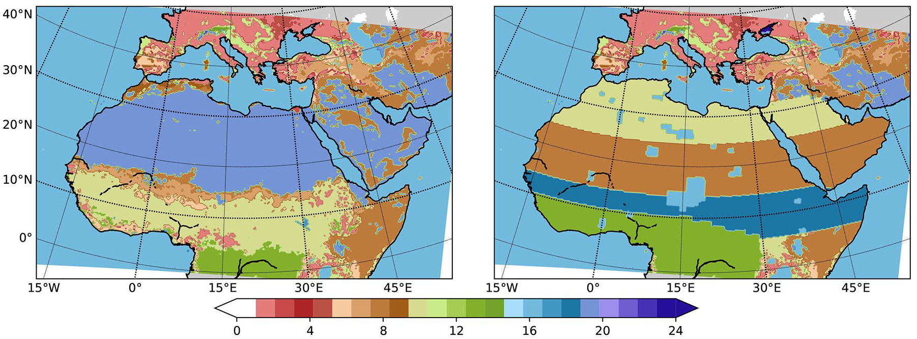
WRF Land Usage index employed for the PI-REF/MH-REF/MH-GSB (left, without surface usage modification) and MH-GSS (right, with surface usage modification) ensemble. Color scale displayed here are in accordance with the USGS 24 category land surface usage index that WRF uses. Category that the modified land usage profile uses over each region are 10 (Savanna), 9 (Mixed Shrubland/Grassland), 18 (Wooded Wetland), and 13 (Evergreen Broadleaf Forest) from north (Mediterranean coast) to south (tropical Africa) across northern Africa.

To assist with the research goals of this study, we have completed four coupled atmosphere-ocean dynamically-downscaled physics ensembles for the MENA region, each containing three members (see Sect. 2.2 for further details on the ensemble members). The first ensemble is configured for the Pre-Industrial (PI) period (and henceforth referred to as RCMPIREF, or PI-REF in short), which serves as the reference climate state against which we compare the MH climate. The three other ensembles are for the MH period; the first of these, which we refer to here as RCMMHREF, or MH-REF in short, represents a “control mid-Holocene” in which only the orbital and trace gas changes associated with MH conditions are included, and a GCM simulation that also only includes MH orbital and trace gas forcings is used to force this RCM ensemble. The purpose of this ensemble is to understand the influence of downscaling around a MH climate state that does not include any feedback from a Green Sahara land surface.

The second MH ensemble, called RCMMHGSB, or MH-GSB in short, is forced by a GCM simulation that includes land-surface feedbacks associated with a Green Sahara in addition to the MH orbital forcings. However, in the RCM itself we do not make the Green Sahara changes (Sect. 2.3) that are made in the GCM to the land surface in the RCM. Therefore, members of this ensemble only sense the presence of a Green Sahara via the boundary forcing by the GCM and spectral nudging within the RCM (Sect. 2.2). The objective of this ensemble is to assess possible feedback from the influence of Green Sahara back to the RCM domain through boundary forcing. Although the absence of GS in RCM makes this ensemble less interesting, the results in this ensemble are still useful for distinguishing teleconnection influence from GS from direct influences over the Middle East region, and to evaluate whether feedback from GS teleconnections will support or against the development of GS.

The third MH ensemble, named RCMMHGSS, or MH-GSS in short, has in addition to the MH-GSB ensemble the Green Sahara changes in the RCM, so members of this ensemble resolve the full influence of the GS surface. The primary goal of this ensemble is to explore the explicit response of RCM to changes in land surface conditions. Furthermore, given that the GS influences both the proxy reconstructed MH climate records and the RCM simulated MH climate in MH-GSS ensemble, direct comparison between them would validate the quality of RCM simulated MH period climate.

Regional climate models, configurations, and forcing data

The atmospheric component of our coupled dynamical downscaling pipeline is the Weather Research and Forecasting (WRF) model, version V4.1.2, with the Advanced Research WRF (ARW) dynamical core (Skamarock et al., 2019). In this study, WRF is configured as a single domain covering the MENA region at 30 km resolution (Sect. 2.1). Performance of the WRF model over this region has been examined by many studies (e.g. Constantinidou et al., 2020; Klein et al., 2015; Zittis et al., 2014; Zittis and Hadjinicolaou, 2017, to name a few), and recently, we have assessed the performance and suitability of several physics parameterization schemes in WRF for this region (Xie et al., 2023). Based on this, three physics scheme combinations that exhibit good overall performance in reconstructing the modern day climate of the region, named N1, N2, and N5, are continuously employed as RCM configuration of this study. The set of physics schemes all uses the Unified Noah Land Surface Model (Noah-LSM; Chen and Dudhia, 2001); the New Thompson (Thompson et al., 2008); two cumulus schemes, Grell-Freitas (GF; Grell and Freitas, 2014) for N2, N5, or Tiedtke (Tiedtke, 1989) for N1; two planetary boundary layer schemes, Mellor-Yamada-Nakanishi-Niino (MYNN) Level 2.5 (Nakanishi and Niino, 2006, 2009) for N1, N2, or Yonsei University Scheme (YSU) for N5; and two surface layer schemes, MYNN for N1, N2, or Revised MM5 (the fifth-generation Penn state/NCAR Mesoscale Model, Jiménez et al., 2012) for N5. The specific configurations of each ensemble set are documented on Table 1 in the previous study (Xie et al., 2023). All simulations employ the RRTMG shortwave and longwave radiation scheme (Rapid Radiative Transfer Model, updated version (Iacono et al., 2008)), with greenhouse gas concentrations in the atmosphere adjusted to PI level for all PI and MH period simulations. This choice has been made in order to better isolate the influences of the MH period green surface boundary conditions.

Table 1.

Statistical Min, Max, Mean, standard deviation (STD) of the precipitation anomaly (model minus proxy) for MH-GSS ensemble members, ensemble mean, and GCM data averaged over three collections of proxy data points.

	Min	Max	Mean	STD	T-statistics	p-Value
	Precipitation Over all Proxy Data Points (mm/year, 27 data points in total)
N1	−479	931	19.2	386	−0.35	0.73
N2	−494	1058	195	363	1.21	0.23
N5	−564	1229	236	382	1.55	0.13
N-ensemble	−430	998	150	350	0.82	0.41
GCM	−533	1611	59.5	440	N/A	N/A
	Precipitation over continental points (mm/year, 14 data points in total)
N1	−479	931	53.1	450	−0.17	0.87
N2	−211	1058	263	365	1.46	0.16
N5	−157	1229	331	358	2.02	0.055
N-ensemble	−282	998	216	361	1.09	0.28
GCM	−483	488	77.5	277	N/A	N/A
	Precipitation over West Africa coastal points (mm/year, 5 data points in total)
N1	−394	−122	−243	88.1	1.82	0.11
N2	−219	−196	28.9	133	3.90	0.0046
N5	−301	274	2.77	189	3.43	0.011
N-ensemble	−250	116	−88.8	117	3.45	0.0087
GCM	−533	−245	−380	121	N/A	N/A

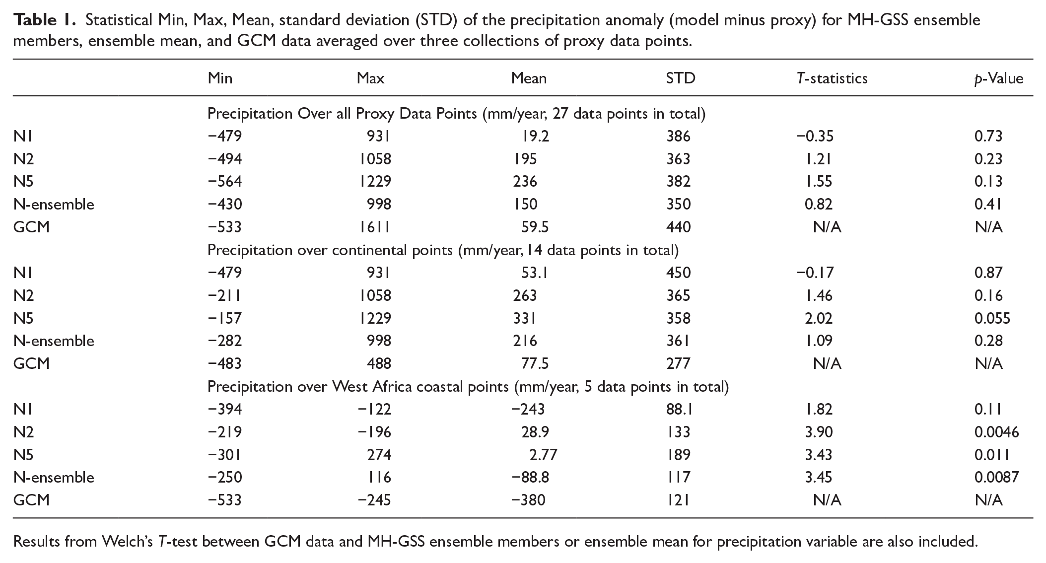
Results from Welch’s T-test between GCM data and MH-GSS ensemble members or ensemble mean for precipitation variable are also included.

The oceanic component of our downscaling pipeline is the Regional Ocean Modeling System (ROMS; Shchepetkin and McWilliams (2005), and the specific version used in this study is Roms Agrif v3.1.1 (Debreu et al., 2012). ROMS regional ocean domain has a horizontal spatial resolution of 0.1 degree. The OASIS3-MCT version 3.0 coupler (Craig et al., 2017) is used to provide online data exchange between WRF and ROMS, and the specific implementation of the coupling is based on the setup used in the Coastal and Regional Ocean COmmunity model (CROCO, Auclair et al. (2018) with technical modifications that are described in Xie et al. (2023). In our configuration, the OASIS coupler interpolates data fields between the atmosphere and the ocean grids using first degree conservative mapping, and the data exchange frequency for all coupled members is set to 1 h.

Though all climate models require initial conditions as inputs, regional models also require boundary conditions. For this study, we used the University of Toronto version of NCAR-CCSM4 (UofT-CCSM4; Peltier and Vettoretti, 2014) to specify the initial and boundary conditions for the atmosphere and ocean regional models. Specifically, we used outputs from the PIREF, MHREF and MHVSL experiments of Chandan and Peltier (2020) corresponding to pre-industrial, MH without Green Sahara and MH with Green Sahara conditions. The results of these experiments have been previously employed to study the MH climate in several other studies (Brierley et al., 2020; Huo et al., 2021, 2022; Tiwari et al., 2023). The PIREF GCM output drives our PI-REF RCM configuration, while outputs from MHREF drive our MH-REF configuration, and outputs from MHVSL drive our MH-GSB and MH-GSS configurations.

The GCM provides WRF with initial and 6-hourly boundary conditions that include atmospheric temperature, wind, humidity and pressure, and provide the land surface (of WRF) with initial conditions including land surface temperature and other assorted land variables. During model runs, the interior of the WRF domain is further forced with GCM pressure, wind, potential temperature, and humidity fields via use of spectral nudging. The spectral nudging method first applies the Fourier transform to the forcing variables to decompose them into wavenumber spectra over the two horizontal dimensions of the regional domain. Then, for each horizontal dimension, waves with wavelengths smaller than half of the regional domain scale are removed. Then variables in the RCM are nudged toward the sum of the remaining wavenumbers, using nudging coefficients that are recommended by the WRF manual and used in Xie et al. (2021). Since the wave field which has larger wavelength represents larger scale features of the variable, using them as nudging target will preserve the large scale features of the GCM forcing variables in the downscaling process. Smaller scale features from the forcing variables, which are represented by wave fields with small wavelengths, are removed before nudging is applied, so the RCM can freely resolve small scale features. This nudging process is applied to vertical levels in the RCM that are above the surface boundary layer. (for a general discussion on the effects of spectral nudging on RCM results, see Alexandru et al., 2009; Omrani et al., 2015; Separovic et al., 2012; von Storch et al., 2000.) ROMS also receives boundary conditions in the form of monthly 3D temperature and salinity fields along the Atlantic boundary from the GCM, while initial conditions are based on the state of Mediterranean in the GCM, with modifications that are described in the next section. Both atmospheric fields and oceanic fields from GCM have a horizontal resolution of 1° × 1°. For further details on the data requirements for the regional model, the reader is referred to Xie et al. (2023).

All ensembles completed in this study employ a spinup period that consists of two phases: The first spinup phase is a single 15-year integration of the atmosphere-ocean coupled system, using boundary forcing from the respective time period and using the bias corrected ocean fields as initial condition. The physics package employed in this initial spinup integration is based upon that which delivered the median bias in the analysis performed under modern conditions (Xie et al., 2023). In the second phase of this spinup process, the ocean model’s state at the end of the initial spinup period is employed as the initial state for each of the three 15 years long ensemble members. The first 5 years of each of these three distinct integrations are then considered to represent the final spinup phase for each ensemble member. The last 10 years of each of the three ensemble members are then employed as a basis for analysis. The purpose of the first spinup phase is to equilibrate the state of the ocean originated from GCM results with the RCM simulated overlying atmosphere. The purpose of the second spinup phase is to smoothly transition between the impacts of the different physics packages. Given this design, each ensemble will contain 45 model years of data, within which 30 years of data will be employed for analysis. The time scale employed in our spinup process is in close accord to the time scale used in other studies (Akhtar et al., 2018; Sevault et al., 2014).

MH specific adjustments to the regional models

To apply the downscaling mechanism for the time periods involved in this study, namely the pre-industrial and the Mid-Holocene, changes needed to be made concerning orbital parameters and trace gas concentrations to make them appropriate for those time periods. Here, we have applied the same changes to those parameters in WRF as that which have been applied in the GCM simulations of Chandan and Peltier (2020) and which are based on the PMIP Phase 4 (PMIP4; Otto-Bliesner et al., 2017) protocol for the MH simulations. Since ROMS obtains downwelling radiation at the sea surface directly from WRF via the coupler, no orbital parameter related changes in ROMS were necessary. Based on comparison with observational records (Boyer et al., 2019), it was shown in Xie et al. (2023) that the GCM salinity field is biased, therefore a simple bias correction was applied to the MH period salinity initial conditions of the ocean, by scaling the MH salinity from with the ratio between modern period GCM salinity and modern period observed salinity from World Ocean Atlas (WOA, Boyer et al., 2019). The equation to compute bias correction is below:

\begin{array}{l} M H S A L T_{c o r r e c t e d} = M H S A L T_{G C M} \times \\ (W O A S A L T / M O D E R N S A L T_{G C M}) \end{array}

The salinity initial condition for the PI period is also bias corrected using the same method.

As noted above, it is well known that during the MH, the presently desertified regions of northern Africa and the Arabian Peninsula had extensive vegetation cover and contained several large inland water bodies. Such a significant change in the land surface would have altered the energy and moisture balance in the region and would have exerted significant feedback on the climate system (Chandan and Peltier, 2020). Therefore the land surface fields that represent Green Sahara (GS) conditions in MH_VSLGCM are implemented in the RCM domain for the MH-GSS ensemble. These land surface fields include surface albedo, leaf area index, soil type, and associated clay and sand fractions. In particular the land usage type over RCM domain is modified to replicate changes in plant functional type and insertion of lakes that were present in MH_VSLGCM simulation, as documented in Chandan and Peltier (2020). Results of these modifications of land surface conditions are illustrated in Figure 1.

Results

Before presenting MH period results, it is worth reviewing the performance of the coupled RCM on the modern climate over the domain of interest, which is validated in Xie et al. (2023). This study had found that the N physics sets all possess winter season 2 m surface air temperature (T2) biases that are cold over North Africa (~ −3°C) but very close to zero over the Mesopotamia and Levant regions of the Middle East. Summer season T2 biases are connected with precipitation biases, which vary between members from hot and dry (~ +1°C, −1 mm/day for member N1) to cold and wet (~ −1°C, +1.5 mm/day for member N5) which strongly depends on the choice of cumulus scheme employed in WRF. ROMS is able to resolve modern period SST that are mostly within 1°C of the observational record. We concluded in this study that the WRF-ROMS coupled RCM resolves modern climate with acceptable accuracy, suggesting that the model would provide an excellent basis for the analysis of MH climate.

In this study, unless noted otherwise, anomalies of all our MH simulations, RCM or GCM, are defined as changes against the corresponding PI reference configurations. Anomalies between any two ensembles are always computed between members that have the same physics configuration in each ensemble, and ensemble means are computed as the arithmetic mean of the three ensemble members.

The MH-reference ensemble

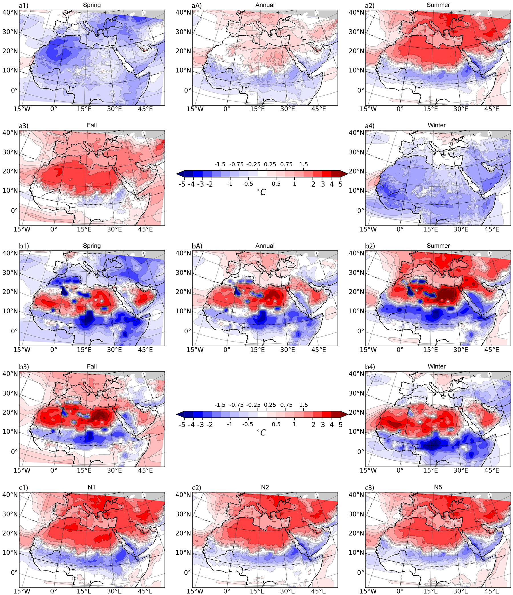
The seasonally and annually averaged T2 anomalies of the MH-REF ensemble, as well as the anomaly between the GCM simulations used for forcing the MH-REF and PI-REF configurations are displayed in Figure 2. The results show clear seasonal variations in T2, with simulated winter and spring season T2 ~1–2°C lower over all land surface within the WRF domain, and summer and fall season T2 ~1°C higher over regions poleward of 20°N. The main driver of this simulated seasonal temperature anomaly is the change in MH period orbital parameters (Berger, 1978; Otto-Bliesner et al., 2017), which modify the incoming solar radiation such that insolation in the northern hemisphere increases during the summer season and decreases during the winter season. Since identical insolation changes are made within the RCM and the GCM, it is unsurprising that large scale spatial patterns in seasonal T2 anomalies are similar between the two. Meanwhile, the decrease in summer temperature over 10–20°N, despite an increase in summer insolation, is due to the increase in monsoonal precipitation (discussed below) which leads to extensive cloud cover and evaporative cooling. This local effect on T2 below 20°N depends on the physics schemes employed in the RCM atmospheric component, WRF (also in Figure 2), and is stronger in member N1 which was found to have a warm and dry bias during the modern period (Xie et al., 2023), and which are therefore most influenced by the effects of precipitation changes.

Figure 2.

Near surface temperature (T2) differences between the MH-REF and the PI-REF RCM ensemble averages (a1–a5), and between the GCM simulations that drive the two ensembles (b1–b5), during various seasons of the year. Summer season T2 differences between each ensemble members of MH-REF and PI-REF ensemble are displayed in (c1–c3).

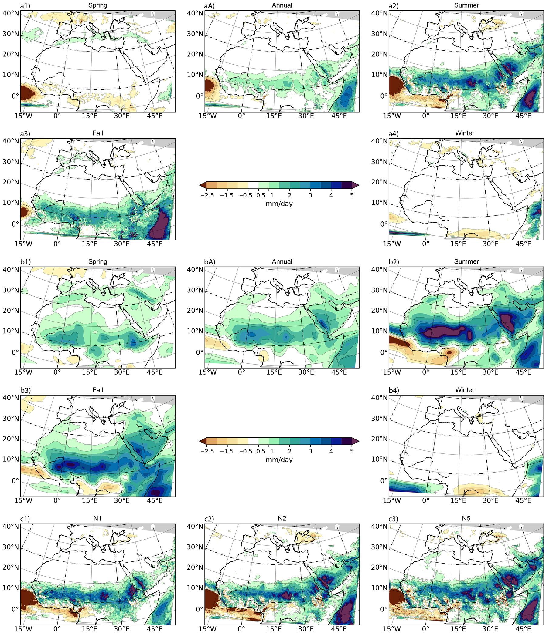
The seasonal mean precipitation change in ensemble members that employ MH-reference forcing is displayed in Figure 3. Over the northern Africa region, all members are characterized by a substantial increase in precipitation during summer season. The highest increase does not occur over regions that observed most precipitation during the modern period, known as the tropical rainbelt between 5 and 10°N (Nicholson, 2009). Rather the strongest increase is located between 10 and 20°N over North Africa and Yemen,indicating a northward expansion of this tropical Rainbelt. The driver of precipitation increase resides in both temperature increase from increased insolation (which leads to stronger low-pressure over land) and MH period circulation changes communicated to the RCM by the GCM via spectral nudging. Therefore, it is unsurprising to find that RCM results are quite similar to GCM results on the large scale. Meanwhile, changes to RCM precipitation are slightly larger in magnitude than GCM. The explanation of this difference resides within the physics schemes employed in WRF, since these physics schemes in the RCM were found to produce more precipitation than in the GCM during the modern period (Xie et al., 2023). Variations in the magnitude of precipitation change between ensemble members, in the summer season (also in Figure 3) during which precipitation increases most, are not large but they are noticeable. These variations are directly related to the configuration of WRF physics schemes, wherein cumulus and microphysics schemes exert strong influence on local precipitation. The influence of physics schemes on precipitation in the MENA region is discussed in Xie et al. (2023), and members that were found to have a positive precipitation bias during the modern period in that study are also found to simulate a larger increase of precipitation during the MH period. The ensemble mean precipitation anomaly (Figure 3) is characterized by the fact that precipitation increase also occurs during fall season over North Africa, during winter season over the eastern coasts of the Adriatic Sea, Black Sea, and the Atlantic Ocean, and slightly during spring season over Sicily, Greece and Syria. These seasonal precipitation increases are mainly controlled by seasonal temperature changes in both the atmosphere and ocean surface, which are driven by MH period insolation. These insolation anomalies also drive the precipitation decrease over tropical regions during the winter and spring season through decrease of incoming radiation during those times.

Figure 3.

Precipitation anomalies (compared to PI-REF) in the MH-REF RCM ensemble averages (a1–a5), and between the GCM simulations that drive the two ensembles (b1–b5), during various seasons of the year. Summer season precipitation anomalies in each members of MH-REF ensemble are displayed in (c1–c3).

Our analysis thus far demonstrates that both the precipitation and T2 fields are similar between the RCM and the GCM in terms of large scale features and seasonality. This demonstrates that the modifications to the RCM that enable it to simulate the MH time period were successful in that GCM results are accurately replicated in RCM but at higher spatial resolution, since other boundary conditions and land surface conditions are unchanged for the MH-REF ensemble. Furthermore, good agreements in T2 and precipitation features are found when comparing MH-REF results with either results from Brayshaw et al. (2011) that use a similar “control mid-Holocene” model setup, or with results from PMIP4 ensemble averages analyzed in Brierley et al. (2020). For example, the MH period insolation induced changes in T2 are observed in all three studies, including a ~1ºC decrease in the winter season over northern Africa and a ~1°C warming in the summer season over regions north of 20°N . The ~1 mm/day increase in precipitation and the corresponding decrease in T2 over equatorial Africa during the summer rain season are also observed in all three studies. The consistency between results of our MH-REF ensemble and results from other GCM studies supports our conclusion that our adjustments in the RCM for the “control mid-Holocene” setup have been properly implemented.

MH-GSB ensemble

We will begin here as in the previous subsection by discussing the T2 anomaly. Compared with results for MH-REF, it is seen that in the case of the MH-GSB ensemble (Figure 4), T2 has a notably stronger climate change signal across all seasons: winter and spring season temperatures are slightly increased across the entire domain, while summer and fall seasons are characterized by an even greater increase in T2 over the northern parts of the domain. Summer T2 over the 10–20°N band decreases compared to MH-REF because of a further increase in monsoonal precipitation. However, the climate change signal in RCM T2 for the average over members of the MH-GSB ensemble is not as strong as the signal in the GCM in which the magnitude of change during the summer season is larger. Furthermore, in the GCM the land surface over North Africa is warmer than PI during all seasons of the year, instead of being colder in winter and spring seasons, as in the RCM. Given that none of the RCM ensemble members has these features, as shown in Figure 4 summer season T2 anomaly for each RCM member at the bottom, it is clear that these differences are due to the GS land surface conditions that are included in the GCM. In particular, greening of the land surface of northern Africa decreases the surface albedo in the GCM leading to a warmer T2 over Sahara, while in the equatorial regions, enhanced evaporation from additional vegetation leads to an increase in precipitation and then to additional cooling over these locations. Additionally, in the GCM the added historical water bodies (Chandan and Peltier, 2020) clearly influence T2 above and around them. Given that the MH-GSB configuration does not incorporate the land surface conditions used in the corresponding GCM simulation (Sect. 2.3), it is not surprising to see that our coupled-RCM model simulates a weaker climate change signal. Meanwhile, the seasonal climate change signal in MH-GSB is still stronger than those in the MH-REF as seen in the RCM ensemble average and in results for each ensemble member, indicating that alterations in the global scale climate from GS condition in the GCM are sufficient to enforce a regional climate change signal.

Figure 4.

T2 differences (compared to PI-REF) in the MH-GSB RCM ensemble averages (a1–a5), and between the GCM simulations that drive the two ensembles (b1–b5), during various seasons of the year. Summer season T2 differences in each members of MH-GSB ensemble are displayed in (c1–c3).

Precipitation fields simulated by the RCM system in the MH-GSB ensemble are presented in Figure 5. Comparing with results from the MH-REF ensemble, it is clear that summer season precipitation increases further from the already humid MH period condition that were simulated with insolation increase only. Not only does total precipitation increase between the 10 and 20°N zone over northern Africa, the region experiencing humid conditions also expands slightly northward and significantly eastward toward the southern part of the Arabian peninsula and southern Iran. The same figure shows that ensemble members with wet bias in modern period have more precipitation increase in the MH-GSB ensemble results, similar to what was seen with MH-REF. However, the differences between members in the MH-GSB ensemble are smaller than those in the MH-REF ensemble. Meanwhile, WRF simulated precipitation increases in the MH-GSB ensemble are notably weaker and covering smaller area than precipitation increases simulated by the GCM. These differences are directly connected to the GS land surface conditions employed in the GCM simulation, in which the land surface over northern Africa is vegetated, thus transpiration effect adds additional moisture into the atmosphere to enhance precipitation. This contrast in precipitation change between the GCM and the RCM is also clear for the spring season when additional precipitation over North Africa is predicted by the GCM but not by the RCM, and for the fall season during which the precipitation increase extends to region north of 20°N in GCM but not in RCM. Little precipitation change occurs in both the GCM and the RCM during the dry winter season, suggesting that potential change in the winter season precipitation anomaly would largely depend on local change in land surface conditions. Interestingly, in the MH-GSB ensemble our coupled RCM also predicts more of precipitation than in MH-REF during spring season over the Mediterranean and the Zagros mountains as in the GCM. This change indicates the circulation features in MH-GSB GCM, which forces the RCM through spectral nudging, have widespread influence on the RCM simulated precipitation field, similar to their influence on near-surface temperature field as discussed earlier. An example of change in the large scale circulation features between each RCM ensemble is displayed in Supplemental Figure 1, available online, which shows summer season average horizontal wind fields from member N2 of each RCM ensemble at 850 and 500 hPa height level. This figure demonstrates that the southwest winds around the gulf of Guinea at 850 hPa height are stronger and extend further north in the results with MH-GSB than in the results with MH-REF. These stronger winds at 850 hPa supply the West African Monsoon with more moisture from the Atlantic Ocean, leading to the observed increase in precipitation in the MH-GSB ensemble. It is known that the West African Monsoon can be influenced by vegetation change in northern Africa (Dallmeyer et al., 2020; Gaetani et al., 2017) and by changes in insolation (Adam et al., 2019), but between the MH-GSB and the MH-REF ensemble there is no difference in vegetation or insolation. Therefore, the reason for the stronger winds in the MH-GSB ensemble is the GS boundary forcing as discussed above. Furthermore, the influence of vegetation is visible in the MH-GSS results as winds are further strengthened because of the GS boundary conditions in MH-GSS ensemble. The difference in the strength and position of the African Easterly Jet is also visible between the three ensembles at 500 hPa height. It is known that the African Easterly Jet is also influenced by surface vegetation Wu et al. (2009), and that the strength of vegetation influence depends on the resolution and the representation of convection employed in the model (Jungandreas et al., 2021, 2023). Our results also demonstrate the influence of surface vegetation on the African Easterly Jet, but the model resolution and the methods used to represent the convection process employed in this study is insufficient to reveal the dependency on convection representation and model resolution.

Figure 5.

Precipitation anomalies (compared to PI-REF) in the MH-GSB RCM ensemble averages (a1–a5), and between the GCM simulations that drive the two ensembles (b1–b5), during various seasons of the year. Summer season precipitation anomalies in each members of MH-GSB ensemble are displayed in (c1–c3).

MH-GSS ensemble

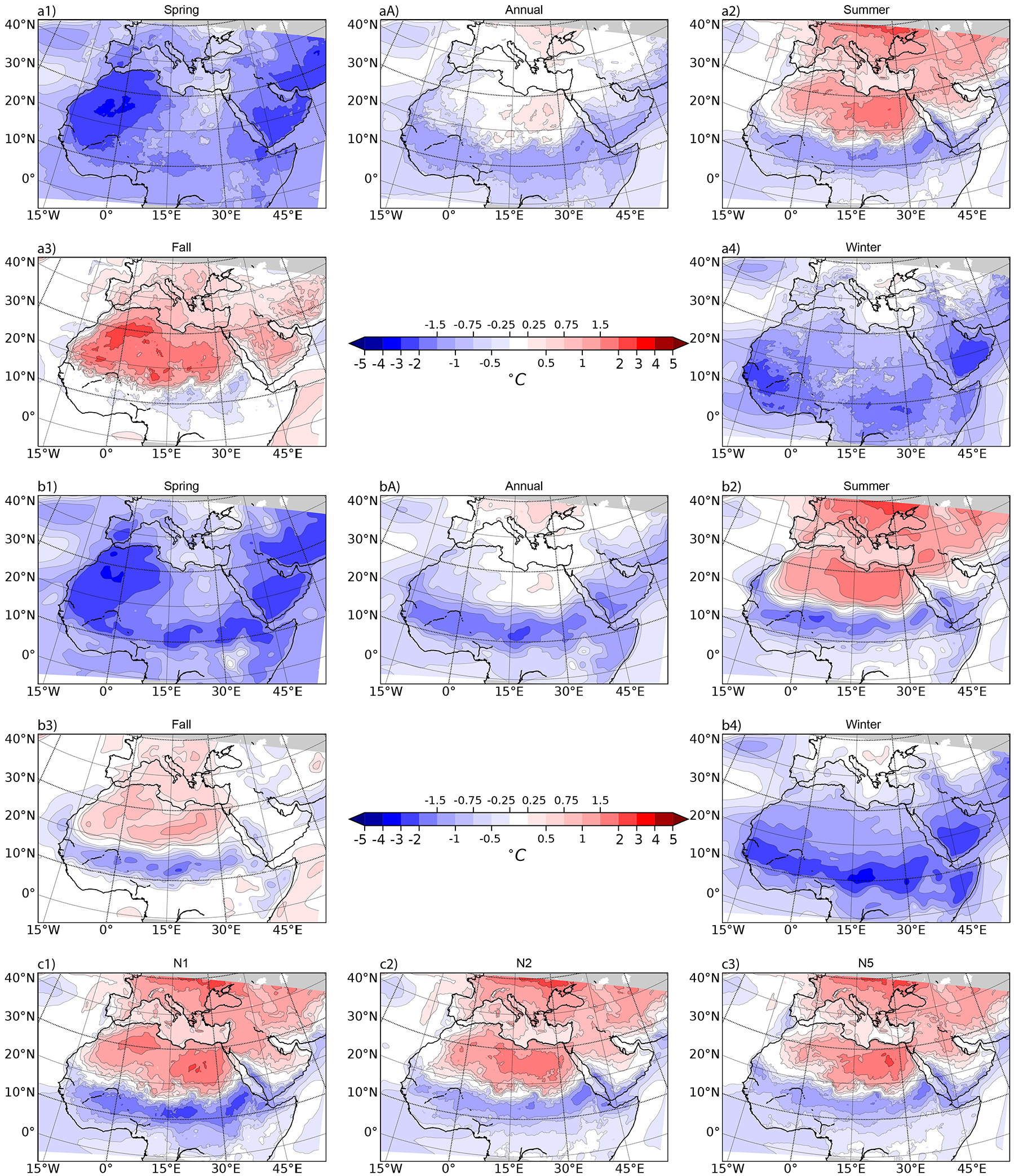
The ensemble mean near surface temperature (T2) from the MH-GSS ensemble is presented in Figure 6 in similar format to results from MH-REF and MH-GSB ensembles. The impacts of the GS surface conditions are clearly visible across the entire RCM domain, and for all seasons. Over the North Africa region T2 changes can be separated into a northern region over the Sahara and a southern region over the Sahel: the southern region is characterized by negative T2 anomalies throughout the year and is especially cold during the winter and spring seasons, while the northern region has a positive T2 anomaly throughout the year. This distinctive difference between the regions is directly related to changes inland surface conditions, as the modified land surface conditions over the southern region contain more forest-type vegetation, while the northern region has more shrub-type vegetation. The region covered by forests would effectively lower local T2 by supporting stronger evapo-transpiration processes that transport heat upward from near-surface level, and provide more moisture to enhance local cloud and precipitation activities, which will be supported by a discussion about precipitation anomaly in the MH-GSS ensemble below. Shrubs, on the other hand, also support the evapo-transpiration process but are weaker than the same process in forested regions. Thus, the northern shrub region sees a lower T2 fall and a lower precipitation increase. Another effect from the greening of land surface is that both forests and shrubs have lower surface albedo than barren land, thus surface of northern Africa in the MH-GSS ensemble is heated more easily by radiative effects than in the MH-GSB ensemble. This radiative effect plays a major role over the northern region, effectively reversing winter T2 anomaly from negative in MH-GSB ensemble to positive in MH-GSS ensemble. Meanwhile such effects are weaker over the southern region because increased cloud cover from enhanced evaporation blocks incoming radiation from reaching the surface. When compared with MH_VSLGCM, the T2 anomaly in MH-GSS ensemble mean is qualitatively similar to anomaly in GCM over all seasons. The T2 anomaly in the southern part is slightly lower in MH-GSS than in GCM, a difference that can be explained by the higher precipitation in RCM, as discussed above. Meanwhile, over the Sahara region, the T2 anomaly in the MH-GSS ensemble average is slightly higher than the GCM during the summer and fall seasons and slightly lower during the winter and spring seasons. These differences are consistent with the amplification of the seasonal cycle in the MH-GSB ensemble, suggesting that the coupled RCM system is more sensitive than the GCM when resolving climate changes. The added water bodies over northern Africa also strongly influence T2 above and around them. However, the influence of these water bodies is not fully resolved since this study did not include an explicit lake model. The full influence of water bodies over northern Africa on MH climate is discussed in Specht et al. (2022), Li et al. (2023), Specht et al. (2024). Simulating lakes in GS with a lake model would be a possible future extension of this research.

Figure 6.

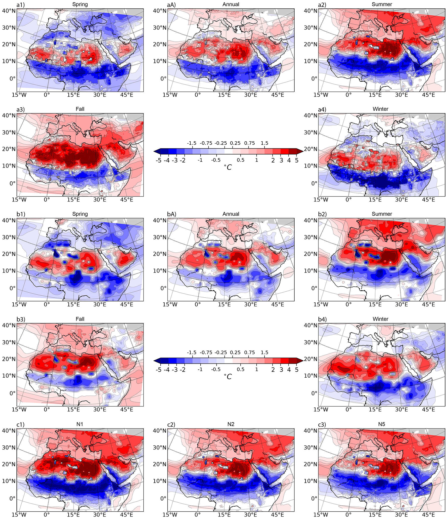
T2 differences (compared to PI-REF) in the MH-GSS RCM ensemble averages (a1–a5), and between the GCM simulations that drive the two ensembles (b1–b5), during various seasons of the year. Summer season T2 differences in each members of MH-GSS ensemble are displayed in (c1–c3).

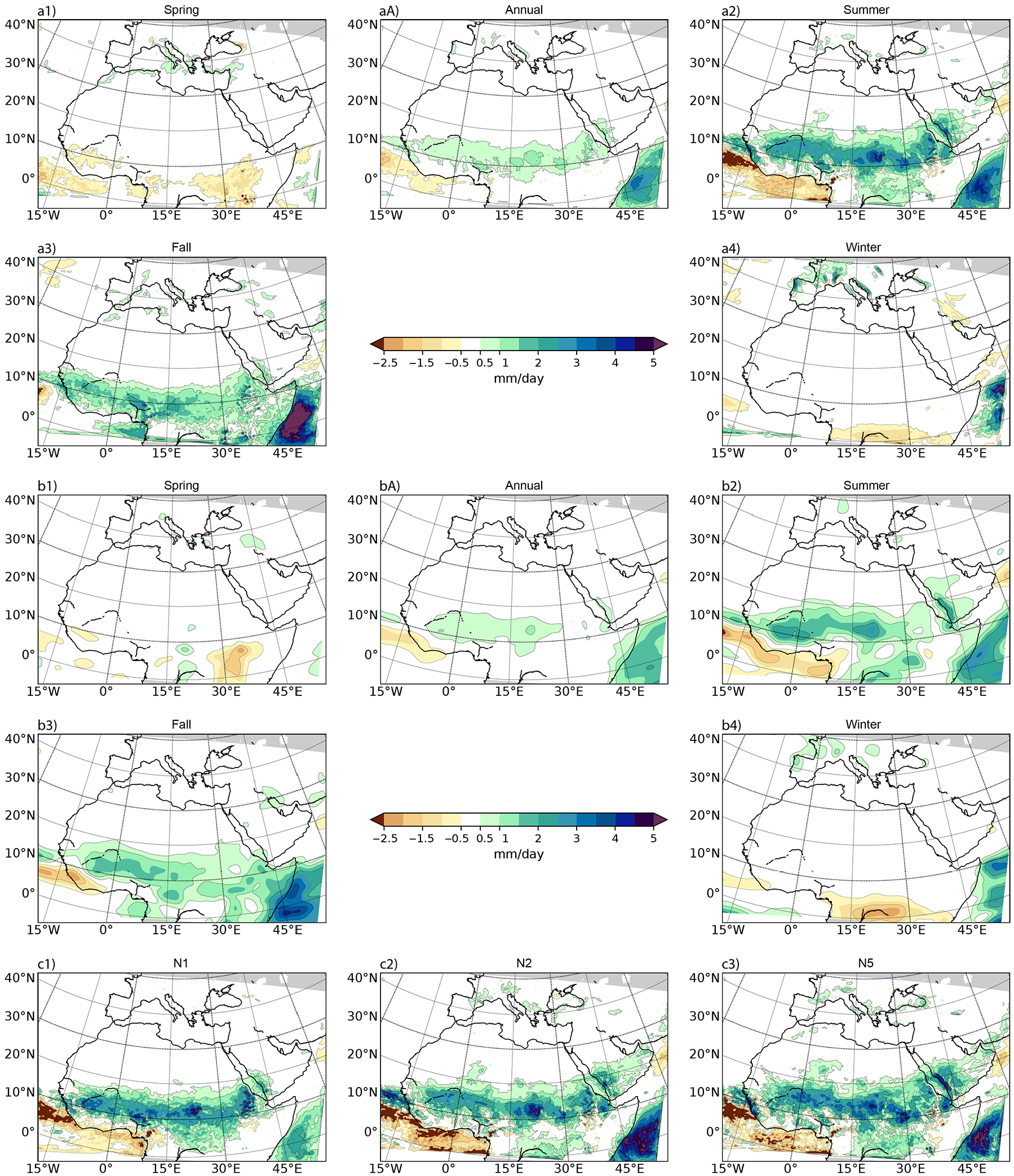
The anomalies in ensemble mean precipitation from the MH-GSS ensemble, averaged annually and over each season, are presented in Figure 7. It is clear that precipitation anomaly in MH-GSS ensemble greatly increases from MH-GSB ensemble across almost all regions over the WRF domain, both annually and over all but the winter season. The strongest increase of precipitation is located between 10 and 20°N over northern Africa and Yemen, where precipitation already increases in the MH-GSB ensemble and is now significantly stronger in the MH-GSS ensemble during the summer and fall seasons, indicating a northward expansion of this tropical rainbelt located between 5 and 10°N in the other two ensembles (Nicholson, 2009). Other regions of the WRF domain experiences different seasonality of precipitation anomaly increase: over the Maghreb region the increase is uniform across spring, summer and fall seasons; over the Zagros mountains the time of precipitation increase is concentrated over the spring season; over the Mediterranean Sea surface precipitation increase is observed during the spring and fall seasons; and along the eastern coast of Tyrrhenian Sea and Adriatic Sea precipitation increase occur during the spring, fall and winter seasons. Compared with precipitation anomalies from the MH_VSLGCM experiment, agreements in seasonal variations are predicted over most regions within the RCM domain, across most seasons, except for two noticeable differences during the summer and fall seasons: The precipitation anomaly in the RCM is stronger than that in the GCM over the tropical rainbelt, but weaker over the Mesopotamia regions. The former is because the coupled RCM is found to be more sensitive to changes than GCM (Xie et al., 2023), while the latter occurs because moisture supply to those regions is heavily sourced from the Arabian Sea, which is not fully covered by the RCM regional domain.

Figure 7.

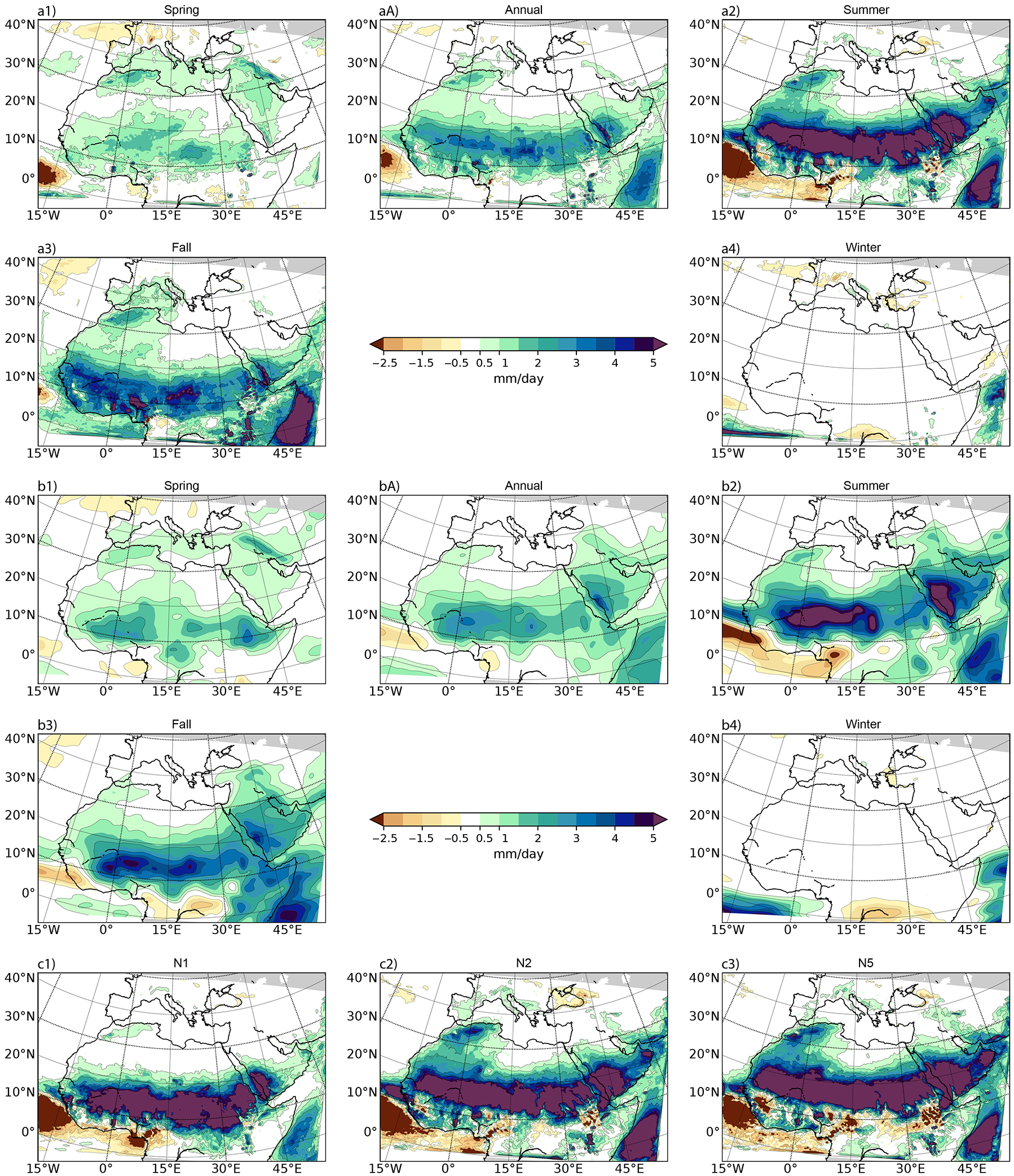
Precipitation anomalies (compared to PI-REF) in the MH-GSS RCM ensemble averages (a1–a5), and between the GCM simulations that drive the two ensembles (b1–b5), during various seasons of the year. Summer season precipitation anomalies in each members of MH-GSS ensemble are displayed in (c1–c3).

Variations in the summer T2 anomaly between members of the MH-GSS ensemble are also larger than those in the MH-REF or MH-GSB ensembles, in both T2 and precipitation as demonstrated in Figures 6 and 7. The T2 anomaly in member N1 is higher over the northern region and lower over the southern region than the other two members. This variation is connected to variation in precipitation, of which member N1 having lower amount than the other two members. Lower precipitation in this member leads to lower evaporation over the northern region that leads to higher T2, and lower consumption of transported moisture over the southern region leads to increased cloudiness over these areas, then to lower T2 via cloud reflection of incoming radiation. The dry bias of N1 member is also characteristic of results for the modern period, in Xie et al. (2023) which demonstrated that the cause of this dry bias is due to the cumulus and microphysics schemes employed in WRF. The repetitive appearance of dry bias in member N1 across all ensembles analyzed in this study confirms this source of bias, since combination of physics schemes has not been altered in this study. Therefore, larger variations between members in the MH-GSS ensemble originate from the greener North Africa surface, over which the wet members deviate further from the dry members due to their difference in the efficiency when increased moisture supply from greener surface is converted to precipitation.

Observing a significant change from employing a GS surface in RCM should not be surprising, as several studies have already pointed out that the increase in vegetation in northern Africa strongly influences the local climate, By using climate models that prescribe a GS surface (Brayshaw et al., 2011; Pausata et al., 2016) or that simulate the greening of the Sahara region with a dynamical vegetation model (Berntell and Zhang, 2024; Dallmeyer et al., 2020). Important influences from the GS surface include an increase in summer season precipitation, a northward expansion of the tropical rainbelt, and the associated decrease in summer season T2. These features are clearly observed in the results of the MH-GSS ensemble, which is consistent with the findings of previous studies and suggests that the GS surface change employed in this ensemble correctly replicates the GS surface in Chandan and Peltier (2020). Furthermore, similarity with other modeling studies alone is not enough to validate our RCM results, since there are uncertainties associated with each specific model Brierley et al. (2020), Marshall et al. (2024), the GS surface representation they use Pausata et al. (2016), Zhang et al. (2021), and even the resolution of the model Jungandreas et al. (2023). Therefore, our RCM results need to be compared with proxy reconstructed climate of the MH period to further examine its quality.

Comparison with MH climate proxies, and latitudinal changes of precipitation over northern Africa

Records of MH period climate can be obtained by reconstructions of various climate proxies, and these reconstructions are widely used to access the quality of climate simulations for past time periods. With up-to-date proxy datasets (Kaufman et al., 2020b; Williams et al., 2018, for example), reconstructions of MH period climate are analyzed at either global scale Kaufman et al. (2020a), Erb et al. (2022), Kaufman and Broadman (2023) or over a local region of interest (Cruz-Silva et al., 2023; Finné et al., 2011, 2019; Jacobson et al., 2024; Mauri et al., 2015). However, the available proxy datasets for the MH period over northern Africa provide only limited spatial resolution. Among these proxy datasets, the one that has the best spatial coverage over northern Africa is of Bartlein et al. (2011). This dataset is based on pollen and plant macrofossil data collected from a variety of sources, which are employed to infer mean annual temperature and precipitation during 6 ka before present (BP), and 21 ka BP. Then the collected data are transformed onto a regular longitude-latitude grid at 2 ° spatial resolution by appropriately averaging over the available data. The broad range of pollen and macrofossil records combined in this dataset provide it an advantage in spatial coverage over northern Africa. This dataset also provides an estimate of the climate anomaly between the 6 and 0 ka BP time periods based on reconstruction studies when possible and on historical climatology dataset otherwise. Therefore this dataset will be used as the target on the basis of which to evaluate the quality of our model simulations.

Comparison between proxy records and model simulations is presented in Figure 8, in which MH anomalies relative to PI for both averaged T2 temperature and precipitation fields from the MH-GSS ensemble mean and GCM data employed in this study are presented with proxy inferences from Bartlein et al. (2011) within the RCM domain. This figure shows good agreement between the MH-GSS ensemble mean and the proxy reconstructed climate in both the precipitation and T2 fields, with RCM results matching or exceeding the amount of precipitation increase seen in proxy reconstructed climate over northern Africa, and matching the T2 increase over the Sahara region. Note that these features are absent in the MH-REF and the MH-GSB ensemble as discussed in earlier sections. Therefore the MH-GSS ensemble outperforms the other two ensembles in terms of closeness with proxy reconstructed climate, primarily due to the GS land surface conditions it employs. A direct comparison between the RCM ensemble means and the proxy reconstructions is provided in Supplemental Figure 2, available online.

Figure 8.

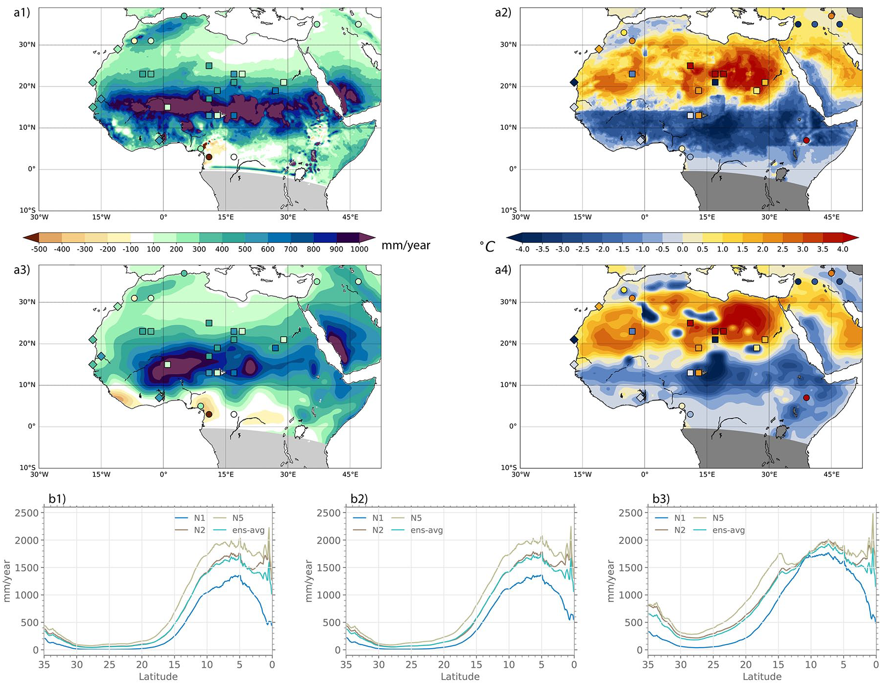
Annual mean anomaly (with respect to PI period results) from proxy reconstruction and model results for precipitation (a1, a3) and T2 (a2, a4) fields. Top row (a1, a2) contains results from the MH-GSS ensemble mean, middle row (a3, a4) contains GCM results. The sub-region that covers inland region of the North Africa Continent are highlighted by square shape, and the sub-region that covers the Atlantic coast of West Africa are highlighted by diamond shape. Circle shape points are data that are included in the all region average but not in the two subregion. Zonally and annually averaged precipitation over land surface of North Africa in each RCM ensemble are presented at bottom row (b1–b3) for the MH-REF ensemble (b1), MH-GSB ensemble (b2), and MH-GSS ensemble (b3).

Meanwhile, the difference between the RCM MH-GSS ensemble mean and the GCM results is smaller in Figure 8, since they both use the same land surface conditions, which leads to similar spatial features in precipitation and T2 between them. To better understand the difference between the downscaled RCM results and the GCM results, data subsets are gathered from grid points closest to each proxy data points for each ensemble member, ensemble average, and GCM results. Since the proxy dataset has a spatial resolution of 2°, data point from the RCM are averages over a region of 7 × 7 grid cells centered at the grid point closest to each proxy data points to better capture the difference in spatial resolution, while data from the GCM are taken directly from the closest grid point. Then the anomalies (model minus proxy) from these data points are computed, and the statistical mean and standard deviation (STD) of these anomalies are displayed in Table 1 for precipitation and in Table 2 for T2. The statistical mean from the RCM ensemble average demonstrates that they have slightly higher precipitation than the GCM results, primarily from member N2 and N5 that are known to have higher precipitation levels as discussed in Section 3.3. Averaged T2 anomalies from the RCM are of smaller magnitude and are positive in sign compared to the negative anomaly from the GCM. In particular, members N2, N5 achieves a smaller than 0.1°C averaged anomaly. In general, closeness in mean value between model simulated results and proxy records suggests that the RCM has the advantage in model performance. However, these differences in anomaly between the RCM and the GCM are not excluded from randomness within each dataset, which can be evaluated using Welch’s T-test (Welch, 1947). Results from this statistical test are characterized by p-values greater than 0.1, and a large p-value (large in T-test is usually defined as greater than a threshold of 0.1 or 0.05) in the Welch’s T-test means that the differences in the mean value could come from randomness in the data samples. This is unsurprising, because the collection of proxy data points covers the Sahara region, the Maghreb region, and the Sahel region, which all have their own climate characteristics that are not necessarily the same. Combining all of these regions together leads to increased randomness in the dataset, which is captured by the T-test.

Table 2.

Statistical Min, Max, Mean, standard deviation (STD) of the T2 anomaly (model minus proxy) for MH-GSS ensemble members, ensemble mean, and GCM data averaged over three collections of proxy data points.

Ensemble Name	Min	Max	Mean	STD	T-statistics	p-Value
	T2 over all proxy data points (°C, 23 data points in total)
N1	−6.51	7.57	0.43	3.32	1.08	0.29
N2	−6.26	6.85	0.076	3.20	0.75	0.46
N5	−6.17	6.70	−0.0084	3.15	0.67	0.51
N-ensemble	−6.32	7.04	0.17	3.21	0.84	0.41
GCM	−6.79	5.54	−0.69	3.56	N/A	N/A
	T2 over continental points (°C, 10 data points in total)
N1	−4.37	7.57	0.65	3.49	1.37	0.19
N2	−3.95	6.85	0.16	3.25	1.13	0.27
N5	−3.94	6.70	−0.040	3.18	1.02	0.32
N-ensemble	−4.09	7.04	0.26	3.30	1.18	0.25
	T2 Over West Africa coastal points (°C, 4 data points in total)
GCM	−6.78	5.54	−1.81	4.10	N/A	N/A
N1	−1.74	5.68	0.99	2.92	−0.047	0.96
N2	−2.18	5.60	0.81	2.96	−0.035	0.97
N5	−2.07	5.32	0.85	2.79	−0.020	0.98
N-ensemble	−2.00	5.53	0.88	2.89	−0.0024	0.998
GCM	−1.69	4.54	0.89	2.27	N/A	N/A

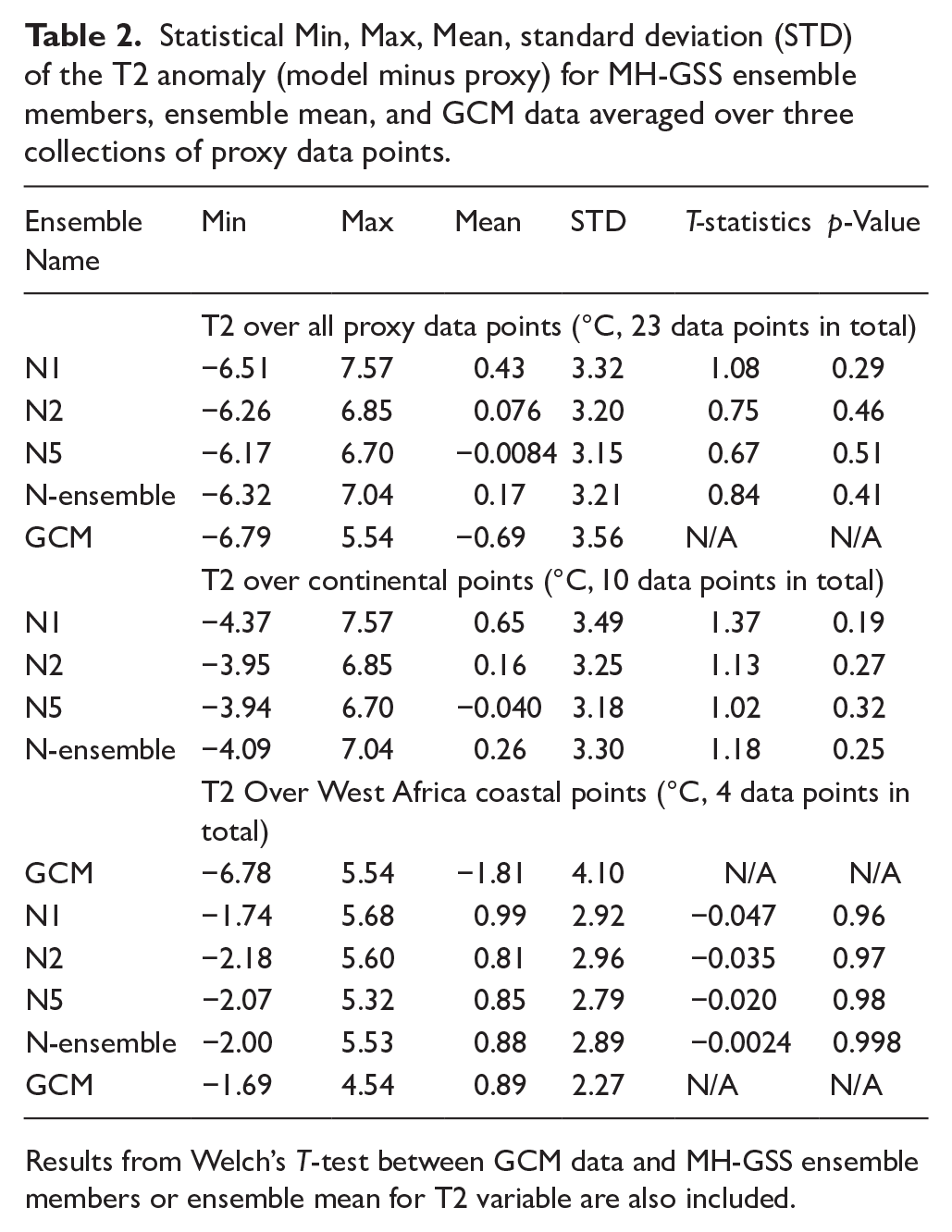
Results from Welch’s T-test between GCM data and MH-GSS ensemble members or ensemble mean for T2 variable are also included.

In order to avoid averaging over regions with different anomaly type, we define two sub-regions: the first consists of all inland regions of northern Africa, and the second consists of regions close to the western coast. These two regions are denoted by square and diamond shapes in Figure 8. The statistical mean, STD, and Welch’s T-test results are also computed for these two sub-regions and presented in Table 1 for precipitation and in Table 2 for T2. Results from the continental region are similar to results obtained for the all location average, where the RCM results are characterized by higher precipitation and higher T2 than the proxy reconstructed values, given by greater than zero values in the regional mean of model minus proxy anomaly, presented in Tables 1 and 2, but these differences are not sufficient to pass the statistical test for significance. However, results for the Atlantic coastal region are characterized by a statistically significant improvement in fit to the proxy records for precipitation predicted by the RCM, characterized by a reduction in the magnitude of model minus proxy difference, but not in T2. The good agreement between simulated T2 is due to the fact that T2 is strongly controlled by both land surface conditions and proximity to the SST fields of the Atlantic ocean. On the other hand, the significant improvement in RCM precipitation compared to GCM precipitation is attributed to the high spatial resolution of the RCM domain, and in particular the resolution of the spatial position of the coastline. The influence of increases spatial resolution is less apparent over inland regions because the prescribed land surface conditions over these regions is at GCM resolution. Additionally, precipitation record reconstructed by Tierney et al. (2017) using leaf wax isotopes showed more than 300mm/year increase in precipitation during the MH period along the coast of Northwest Africa. This magnitude of precipitation increase is matched by members N2 and N5 of the MH-GSS ensemble but not the N1 member or the forcing GCM, as showed by Supplemental Figure 3, available online, suggesting that an RCM may potentially perform better than GCM in resolving MH-GS precipitation over this region.

The zonal averages of the RCM simulated precipitation over the land surface of northern Africa, in the MH-REF, MH-GSB, and MH-GSS ensembles are also shown in Figure 8 in absolute values. The mean feature of zonally averaged precipitation over northern Africa is the tropical rainbelt, defined as a region that has more than 1500 mm/year of zonally averaged precipitation. In the MH-GSS ensemble, the tropical rainbelt region has its northern boundary located at 15°N, a latitude that only has 500 mm/year of precipitation under PI conditions. Therefore, the increase of zonally averaged precipitation between the PI ensemble and the MH-GSS ensemble has a magnitude of more than 1000 mm/year near 15°N latitude. The tropical rainbelt in the MH-REF ensemble has its northern boundary located at 10°N latitude, a location at which there is already a zonally averaged precipitation of more than 1000 mm/year under PI conditions. Therefore, the increase of zonally averaged precipitation in the MH-REF ensemble relative to that in the PI-REF ensemble has a magnitude of only 400 mm/year and does not cover as much latitude as the anomaly in the MH-GSS ensemble. The zonally averaged precipitation field in the MH-GSB ensemble is found to be much closer to that in the MH-REF ensemble than to that in the MH-GSS ensemble. The drastic differences between the MH-GSS ensemble and the other two ensembles are clearly due to the GS land surface conditions in the MH-GSS ensemble that supplies moisture into the atmosphere through evaporation from the vegetated surface. Nevertheless, the northward expansion of the rainbelt is still visible in the two ensembles that do not include GS land surface conditions, which arise due to insolation driven changes of large scale climate features over northern Africa during the MH period. These precipitation increases that occurred in the absence of GS land surface conditions suggest that the insolation change contributed to the onset of Green Sahara. More importantly, the findings in Bonfils et al. (2001) show that at least 200 mm/year of precipitation are required to sustain grasslands over the northern Africa land surface. This level of precipitation increase is observed in both the MH-REF and the MH-GSB ensemble over regions south of 15°N, and in the MH-GSS ensemble over almost all of northern Africa. Therefore, results from the MH-REF and MH-GSB ensembles suggests that changes in insolation forcing would initiate northward expansion of the vegetated region, and results from the vegetated MH-GSS ensemble suggests that the greened surface can sustain itself.

Summary and discussion

In this study, we have presented a series of dynamically downscaled atmosphere-ocean coupled regional climate simulations that represent the MH period climate over the Middle East, Mediterranean and northern Africa regions. For simulations without a direct implementation of GS conditions in RCM, the climate change signals observed in the results are primarily attributable to three factors: The UofT-CCSM4 GCM forcing data during the MH period, both with and without the presence of a GS, that serves as initial and boundary condition for the RCM; the physics schemes employed in the Weather Research and Forecasting (WRF) model; and the orbital insolation regime which is common to both the RCM and the GCM. For RCM simulations that include a GS surface condition, the GS conditions becomes a primary, if not dominant, factor in determining the results of the simulation.

When the reference MH GCM (i.e. without GS land surface conditions) forcing is employed, we find that the climate change signal simulated by the RCM is quite similar to changes in the GCM itself. Changes in orbital parameters would alter the insolation fields with an increase during the summer season and a decrease during the winter season, leading to a rise and fall of near surface temperature (T2) in the respective seasons. Increased temperature during the summer season will also enhance evaporation over water surfaces of the Atlantic Ocean and the Mediterranean Sea, resulting in increases in summer precipitation over northern Africa through moisture transport by winds. MH period insolation fields also lead to northward shift of the tropical rainbelt during the summer season, which is captured by the RCM as a northward expansion of precipitation fields over tropical regions of Africa. When compared across members within the same ensemble, they predicted climate anomalies that are mostly uniform, which is consistent with the finding in Xie et al. (2021) that GCM resolved large scale circulation features are the primary factor determining predicted climate anomalies across different time periods. Variations in physics schemes discussed in Xie et al. (2023) also influence the final RCM results, as ensemble members that have wet bias during the modern period are characterized by higher precipitation anomalies in the MH period simulations than the relatively dryer members.

Climate change signal simulated by the RCM diverges from those of the GCM when the RCM without GS land surface conditions is forced by a GCM simulation that includes GS land surface conditions. The absence of GS land surface conditions in the RCM leads to a weaker precipitation increase in its simulations due to lack of increased evapotranspiration from surface vegetation, and lower winter temperature due to unchanged surface albedo (the desert modern day surface has albedo higher than vegetated land). Nevertheless, the GS GCM forcing still strengthens the RCM predicted climate anomaly that appears as an increases in both precipitation and temperature, compared to those obtained from RCM simulations that employ GCM forcing without GS land surface conditions. This increase of RCM predicted climate anomalies is influenced by large scale circulation features in the GCM forcing data that include GS land surface conditions.

When the GS land surface conditions are employed in the RCM, they have a major influence on the results within the MH-GSS ensemble. These influences include a significant increase of precipitation over the tropical rainbelt, that reaches a level that is much higher than precipitation in the MH-REF or MH-GSB ensembles and that matches or exceeds the GS GCM results. The T2 field from the MH-GSS ensemble also matches GS GCM results by delivering a lower summer temperature over the tropical rainbelt regions and a higher winter temperature over the Sahara region. Since the MH-GSS ensemble differs from the the MH-GSB ensemble only in land surface conditions over the northern Africa, differences between these two ensembles are clearly derived from the greening of the land surface. Variations between members of the MH-GSS ensemble are also amplified by the GS surface condition, as the greener surface leads to more evaporation and thus an increase in the source of precipitation, and the strength of precipitation increase is strongly dependent on the individual cumulus and microphysics schemes employed in each ensemble member.

The inclusion of GS land surface conditions brought RCM results closer not only to the GCM results, but also to the proxy reconstructed climate records during the MH period. The magnitude of precipitation increase and T2 change in proxy reconstruction are matched by results from the MH-GSS ensemble much closer than the other ensembles. The close correspondence between the GCM and the RCM MH-GSS results demonstrates that the transfer of the GS land surface conditions employed in Chandan and Peltier (2020) is properly implemented in the RCM. The GS land surface conditions employed in the RCM also constrains the RCM results, because of their low spatial resolution limits the improvement in RCM results that might otherwise be expected because of the higher spatial resolution of the model. Nevertheless, results from the RCM MH-GSS ensemble are still very close to proxy records. This establishes that our downscaling pipeline is delivering results of high quality for MH climate conditions over northern Africa, the Mediterranean Basin, and the Levant.

When comparing the RCM results obtained in this study with the results from other studies that includes a GS surface, there is good agreement on the influence of the GS. In particular, the inclusion of the GS surface leads to a significant increase in precipitation in the monsoon regions of northern Africa and an increase in T2 over the Sahara region. These features are found in other studies that include a GS surface (Brayshaw et al., 2011; Dallmeyer et al., 2020; Jungandreas et al., 2023; Marshall et al., 2024; Pausata et al., 2016; Zhang et al., 2021), and in our study. When considering the “mid-Holocene temperature conundrum”’ described in Liu et al. (2014), this conundrum is clearly visible in our results without the GS, which is colder than proxy reconstructions. Including GS land surface conditions increases T2 over northern Africa and brings our results closer to proxy reconstructions from Bartlein et al. (2011). Therefore, results from this study can support the conclusion in Kaufman and Broadman (2023) that the “mid-Holocene temperature conundrum”’ can be partially resolved by including changes in terrestrial vegetation, which leads to closer agreement between climate model simulations and proxy reconstructions.

Supplemental Material

sj-pdf-1-hol-10.1177_09596836251350243 – Supplemental material for Mid-Holocene climate over the Mediterranean, North Africa, and Middle East simulated using a regional climate model

Supplemental material, sj-pdf-1-hol-10.1177_09596836251350243 for Mid-Holocene climate over the Mediterranean, North Africa, and Middle East simulated using a regional climate model by Fengyi Xie, Deepak Chandan and William Richard Peltier in The Holocene

Footnotes

Acknowledgements

The simulations presented in this paper were performed on the SciNet High Performance Computing facility at the University of Toronto, which is a component of the Compute Canada HPC platform. The authors would like to thank support team of SciNet, Jonathan Gula, and Valentine Bernu for providing assistance on implementing the CROCO software.

Author contributions

Fengyi Xie: Conceptualization; Data curation; Formal analysis; Investigation; Methodology; Software; Visualization; Writing – original draft; Writing – review & editing.

Deepak Chandan: Conceptualization; Data curation; Investigation; Methodology; Software; Visualization; Writing – original draft; Writing – review & editing.

W. Richard Peltier: Conceptualization; Funding acquisition; Methodology; Project administration; Resources; Supervision; Writing – original draft; Writing – review & editing.

Funding

The author(s) disclosed receipt of the following financial support for the research, authorship, and/or publication of this article: Support for F. Xie has been provided by SSHRC Grant 504343 to T. Harrison and WRP. This research was partially supported by the CRANE project (award 895-2011-1026, Social Sciences and Humanities Research Council, Canada; ).

ORCID iD

Fengyi Xie

Supplemental material

Supplemental material for this article is available online.

Notes

References

Adam

Schneider

Enzel

, et al. (2019) Both differential and equatorial heating contributed to African monsoon variations during the mid-Holocene. Earth and Planetary Science Letters 522: 20–29.

Akhtar

Brauch

Ahrens

(2018) Climate modeling over the Mediterranean Sea: Impact of resolution and ocean coupling. Climate Dynamics 51: 933–948.

Alder

Hostetler

(2015) Global climate simulations at 3000-year intervals for the last 21 000 years with the GENMOM coupled atmosphere–ocean model. Climate of the Past 11(3): 449–471.

Alexandru

De Elia

Laprise

, et al. (2009) Sensitivity study of regional climate model simulations to large-scale nudging parameters. Monthly Weather Review 137(5): 1666–1686.

Arnault

Knoche

Wei

, et al. (2016) Evaporation tagging and atmospheric water budget analysis with WRF: A regional precipitation recycling study for West Africa. Water Resources Research 52(3): 1544–1567.

Auclair

Bordois

Dossmann

, et al. (2018) A non-hydrostatic non-Boussinesq algorithm for free-surface ocean modelling. Ocean Modelling 132: 12–29.

Bader

Jungclaus

Krivova

, et al. (2020) Global temperature modes shed light on the Holocene temperature conundrum. Nature Communications 11(1): 4726.

Barth

(1857) Travels and Discoveries in North and Central Africa, vol. 2. Cambridge: Harper and Brothers.

Bartlein

PJJ

Harrison

Brewer

, et al. (2011) Pollen-based continental climate reconstructions at 6 and 21 ka: A global synthesis. Climate Dynamics 37: 775–802.

10.

Berger

(1978) Long-term variations of daily insolation and Quaternary climatic changes. Journal of the Atmospheric Sciences 35(12): 2362–2367.

11.

Berntell

Zhang

(2024) Mid-Holocene West African monsoon rainfall enhanced in EC-Earth simulation with dynamic vegetation feedback. Climate Dynamics 62(7): 7001–7017.

12.

Bonfils

de Noblet-Ducoudré

Braconnot

, et al. (2001) Hot desert albedo and climate change: Mid-Holocene monsoon in North Africa. Journal of Climate 14(17): 3724–3737.

13.

Boyer

Baranova

Locarnini

, et al. (2019) World Ocean Atlas 2018: Product Documentation. Silver Spring, MD: Ocean Climate Laboratory.

14.

Braconnot

Zhu

Marti

, et al. (2019) Strengths and challenges for transient Mid-to Late-Holocene simulations with dynamical vegetation. Climate of the Past 15(3): 997–1024.

15.

Brayshaw

Rambeau

CMC

Smith

(2011) Changes in Mediterranean climate during the Holocene: Insights from global and regional climate modelling. Holocene 21(1): 15–31.

16.

Brierley

Zhao

Harrison

, et al. (2020) Large-scale features and evaluation of the PMIP4-CMIP6 mid Holocene simulations. Climate of the Past 16: 1847–1872.

17.

Chandan

Peltier

(2020) African humid period precipitation sustained by robust vegetation, soil, and lake feedbacks. Geophysical Research Letters 47(21): e2020GL088728.

18.

Chen

Dudhia

(2001) Coupling an advanced land surface–hydrology model with the Penn State–NCAR MM5 modeling system. Part I: Model implementation and sensitivity. Monthly Weather Review 129(4): 569–585.

19.

Claussen

Dallmeyer

Bader

(2017) Theory and modeling of the African humid period and the green Sahara. In: Oxford Research Encyclopedia of Climate Science. Oxford: Oxford University Press.

20.

Claussen

Gayler

(1997) The greening of the Sahara during the mid-Holocene: Results of an interactive atmosphere-biome model. Global Ecology and Biogeography Letters 6: 369–377.

21.

Constantinidou

Hadjinicolaou

Zittis

, et al. (2020) Performance of land surface schemes in the WRF model for climate simulations over the MENA-CORDEX domain. Earth Systems and Environment 4: 647–665.

22.

Craig

Valcke

Coquart

(2017) Development and performance of a new version of the OASIS coupler, OASIS3-MCT_3.0. Geoscientific Model Development 10(9): 3297–3308.

23.

Cremaschi

Di Lernia

(1999) Holocene climatic changes and cultural dynamics in the Libyan Sahara. African Archaeological Review 16: 211–238.

24.

Cruz-Silva

Harrison

Prentice

, et al. (2023) Pollen-based reconstructions of Holocene climate trends in the eastern Mediterranean region. Climate of the Past 19(11): 2093–2108.

25.

d’Orgeville

Peltier

Erler

, et al. (2014) Climate change impacts on Great Lakes Basin precipitation extremes. Journal of Geophysical Research Atmospheres 119(18): 10799–10812.

26.

Dallmeyer

Claussen

Lorenz

, et al. (2020) The end of the African humid period as seen by a transient comprehensive Earth system model simulation of the last 8000 years. Climate of the Past 16(1): 117–140.

27.

Dallmeyer

Claussen

Lorenz

, et al. (2021) Holocene vegetation transitions and their climatic drivers in MPI-ESM1.2. Climate of the Past 17(6): 2481–2513.

28.

Davis

BAS

Brewer

Stevenson

, et al. (2003) The temperature of Europe during the Holocene reconstructed from pollen data. Quaternary Science Reviews 22(15–17): 1701–1716.

29.

Debreu

Marchesiello

Penven

, et al. (2012) Two-way nesting in split-explicit ocean models: Algorithms, implementation and validation. Ocean Modelling 49–50: 1–21.

30.

Dell’Aquila

Mariotti

Bastin

, et al. (2018) Evaluation of simulated decadal variations over the Euro-Mediterranean region from ENSEMBLES to Med-CORDEX. Climate Dynamics 51: 857–876.

31.

DeMenocal

Ortiz

Guilderson

, et al. (2000) Abrupt onset and termination of the African Humid Period: Rapid climate responses to gradual insolation forcing. Quaternary Science Reviews 19(1–5): 347–361.

32.

di Lernia

(2017) The archaeology of rock art in Northern Africa. In: Bruno D and McNiven IJ (eds) The Oxford Handbook of the Archaeology and Anthropology of Rock Art. Oxford: Oxford University Press, pp.95–121.

33.

Dong

, et al. (2022) The Holocene temperature conundrum answered by mollusk records from East Asia. Nature Communications 13(1): 5153.

34.

Dunne

Evershed

Salque

, et al. (2012) First dairying in green Saharan Africa in the fifth millennium BC. Nature 486(7403): 390–394.

35.

Duque-Villegas

Claussen

Brovkin

, et al. (2022) Effects of orbital forcing, greenhouse gases and ice sheets on Saharan greening in past and future multi-millennia. Climate of the Past 18(8): 1897–1914.

36.

Erb

McKay

Steiger

, et al. (2022) Reconstructing Holocene temperatures in time and space using paleoclimate data assimilation. Climate of the Past 18(12): 2599–2629.

37.

Erler

Peltier

(2016) Projected changes in precipitation extremes for western Canada based on high-resolution regional climate simulations. Journal of Climate 29(24): 8841–8863.

38.

Erler

Peltier

(2017) Projected hydroclimatic changes in two major river basins at the Canadian west coast based on high-resolution regional climate simulations. Journal of Climate 30(20): 8081–8105.

39.

Erler

Peltier

D’Orgeville

(2015) Dynamically downscaled high-resolution hydroclimate projections for western Canada. Journal of Climate 28(2): 423–450.

40.

Essell

Esper

Wanner

, et al. (2024) Rethinking the Holocene temperature conundrum. Climate Research 92: 61–64.

41.

Finné

Holmgren

Sundqvist

, et al. (2011) Climate in the eastern Mediterranean, and adjacent regions, during the past 6000 years – A review. Journal of Archaeological Science 38(12): 3153–3173.

42.

Finné

Woodbridge

Labuhn

, et al. (2019) Holocene hydro-climatic variability in the Mediterranean: A synthetic multi-proxy reconstruction. Holocene 29(5): 847–863.

43.

Fletcher

Debret

Goñi

MFS

(2013) Mid-Holocene emergence of a low-frequency millennial oscillation in western Mediterranean climate: Implications for past dynamics of the North Atlantic atmospheric westerlies. Holocene 23(2): 153–166.

44.

Gabriel

(1987) Palaeoecological evidence from Neolithic fireplaces in the Sahara. African Archaeological Review 5: 93–103.

45.

Gaetani

Messori

Pausata

FSR

, et al. (2024) Mid-Holocene climate at mid-latitudes: Assessing the impact of Saharan greening. Climate of the Past 20(8): 1735–1759.

46.

Gaetani

Messori

Zhang

, et al. (2017) Understanding the mechanisms behind the northward extension of the West African monsoon during the mid-Holocene. Journal of Climate 30(19): 7621–7642.

47.

Giorgi

Jones

Asrar

(2009) Addressing climate information needs at the regional level: The CORDEX framework. World Meteorological Organization (WMO) Bulletin 58(3): 175.

48.

Glotfelty

Ramírez-Mejía

Bowden

, et al. (2021) Limitations of WRF land surface models for simulating land use and land cover change in Sub-Saharan Africa and development of an improved model (CLM-AF v. 1.0). Geoscientific Model Development 14(6): 3215–3249.

49.

Grell

Freitas

(2014) A scale and aerosol aware stochastic convective parameterization for weather and air quality modeling. Atmospheric Chemistry and Physics 14(10): 5233–5250.

50.

Gula

Peltier

(2012) Dynamical downscaling over the Great Lakes basin of North America using the WRF regional climate model: The impact of the Great Lakes system on regional greenhouse warming. Journal of Climate 25(21): 7723–7742.

51.

Harrison

Bartlein

(2012) Records from the past, lessons for the future: what the palaeorecord implies about mechanisms of global change. In: Henderson-Sellers A and McGuffie K (editors) (2012) The Future of the World’s Climate. Boston MA, USA: Elsevier, pp.403–436.

52.

Hoelzmann

Jolly

Harrison

, et al. (1998) Mid-Holocene land-surface conditions in northern Africa and the Arabian Peninsula: A data set for the analysis of biogeophysical feedbacks in the climate system. Global Biogeochemical Cycles 12(1): 35–51.

53.

Hoelzmann

Keding

Berke

, et al. (2001) Environmental change and archaeology: Lake evolution and human occupation in the Eastern Sahara during the Holocene. Palaeogeography Palaeoclimatology Palaeoecology 169(3–4): 193–217.

54.

Holmes

Hoelzmann

(2017) Late Pleistocene-Holocene African Humid Period as Evident in Lakes. Oxford: Oxford University Press.

55.

Hopcroft

Valdes

(2019) On the role of dust-climate feedbacks during the mid-Holocene. Geophysical Research Letters 46(3): 1612–1621.

56.

Hopcroft

Valdes

Harper

, et al. (2017) Multi vegetation model evaluation of the Green Sahara climate regime. Geophysical Research Letters 44(13): 6804–6813.

57.

Hopcroft

Valdes

Shuman

, et al. (2023) Relative importance of forcings and feedbacks in the Holocene temperature conundrum. Quaternary Science Reviews 319: 108322.

58.

Huo

Peltier

(2019) Dynamically downscaled climate simulations of the Indian monsoon in the instrumental era: Physics parameterization impacts and precipitation extremes. Journal of Applied Meteorology and Climatology 58(4): 831–852.

59.

Huo

Peltier

Chandan

(2021) Mid-Holocene monsoons in south and Southeast Asia: Dynamically downscaled simulations and the influence of the Green Sahara. Climate of the Past 17(4): 1645–1664.

60.

Huo

Peltier

Chandan

(2022) Mid-Holocene climate of the Tibetan Plateau and hydroclimate in three major river basins based on high-resolution regional climate simulations. Climate of the Past 18(10): 2401–2420.

61.

Iacono

Delamere

Mlawer

, et al. (2008) Radiative forcing by long-lived greenhouse gases: Calculations with the AER radiative transfer models. Journal of Geophysical Research Atmospheres 113(D13).

62.

Jacobson

Seguin

Finné

(2024) Holocene hydroclimate synthesis of the Aegean: Diverging patterns, dry periods and implications for climate-society interactions. Holocene 34(12): 1807–1823.

63.

Jiménez

Dudhia

González-Rouco

, et al. (2012) A revised scheme for the WRF surface layer formulation. Monthly Weather Review 140(3): 898–918.

64.

Jungandreas

Hohenegger

Claussen

(2021) Influence of the representation of convection on the mid-Holocene West African Monsoon. Climate of the Past 17: 1665–1684.

65.

Jungandreas

Hohenegger

Claussen

(2023) How does the explicit treatment of convection alter the precipitation–soil hydrology interaction in the mid-Holocene African humid period? Climate of the Past 19(3): 637–664.

66.

Kageyama

Braconnot

Harrison

, et al. (2018) The PMIP4 contribution to CMIP6 – Part 1: Overview and over-arching analysis plan. Geoscientific Model Development 11(3): 1033–1057.

67.

Katsafados

Papadopoulos

Korres

, et al. (2016) A fully coupled atmosphere–ocean wave modeling system for the Mediterranean Sea: Interactions and sensitivity to the resolved scales and mechanisms. Geoscientific Model Development 9(1): 161–173.

68.

Kaufman

McKay

Routson

, et al. (2020a) Holocene global mean surface temperature, a multi-method reconstruction approach. Scientific Data 7(1): 201.

69.

Kaufman

McKay

Routson

, et al. (2020b) A global database of Holocene paleotemperature records. Scientific Data 7(1): 115.

70.

Kaufman

Broadman

(2023) Revisiting the Holocene global temperature conundrum. Nature 614(7948): 425–435.

71.

Klein

Heinzeller

Bliefernicht

, et al. (2015) Variability of West African monsoon patterns generated by a WRF multi-physics ensemble. Climate Dynamics 45: 2733–2755.

72.

Kröpelin

(2004) New petroglyph sites in the Southern Libyan Desert. Sahara 15: 111–117.

73.

Larrasoaña

Roberts

Rohling

(2013) Dynamics of green Sahara periods and their role in hominin evolution. PLoS One 8(10): e76514.

74.

Lézine

Hély

Grenier

, et al. (2011) Sahara and Sahel vulnerability to climate changes, lessons from Holocene hydrological data. Quaternary Science Reviews 30(21–22): 3001–3012.

75.

Liu

Jiang

Lang

(2019) Mid-Holocene drylands: A multi-model analysis using Paleoclimate Modelling Intercomparison Project phase III (PMIP3) simulations. Holocene 29(9): 1425–1438.

76.

Liu

Cheng

Zheng

, et al. (2025) The seasonal temperature conundrum for the Holocene. Science Advances 11(17): eadt8950.

77.

Liu

Otto-Bliesner

, et al. (2009) Transient simulation of last deglaciation with a new mechanism for Bolling-Allerod warming. Science 325: 310–314.

78.

Liu

Zhu

Rosenthal

, et al. (2014) The Holocene temperature conundrum. Proceedings of the National Academy of Sciences of the United States of America 111(34): E3501–E3505.

79.

Kino

Cauquoin

, et al. (2023) Contribution of lakes in sustaining the Sahara greening during the Mid-Holocene. Climate of the Past 19(10): 1891–1904.

80.

Miller

Zhang

, et al. (2018) Dynamic vegetation simulations of the mid-Holocene Green Sahara. Geophysical Research Letters 45(16): 8294–8303.

81.

Mackay

Battarbee

Birks

, et al. (eds). (2003) Global Change in the Holocene. London: Arnold, pp.1–528.

82.

Manning

Timpson

(2014) The demographic response to Holocene climate change in the Sahara. Quaternary Science Reviews 101: 28–35.

83.

Marcott

Shakun

Clark

, et al. (2013) A reconstruction of regional and global temperature for the past 11,300 years. Science 339(6124): 1198–1201.

84.

Marshall

Morrill

Dee

, et al. (2024) Causes of past African temperature change in PMIP simulations of the mid-Holocene. Paleoceanography and Paleoclimatology 39(5): e2023PA004706.

85.

Mauri

Davis

BAS

Collins

, et al. (2015) The climate of Europe during the Holocene: A gridded pollen-based reconstruction and its multi-proxy evaluation. Quaternary Science Reviews 112: 109–127.

86.

Nakanishi

Niino

(2006) An improved Mellor–Yamada level-3 model: Its numerical stability and application to a regional prediction of advection fog. Boundary-Layer Meteorology 119: 397–407.

87.

Nakanishi

Niino

(2009) Development of an improved turbulence closure model for the atmospheric boundary layer. Journal of the Meteorological Society of Japan. Ser. II 87(5): 895–912.

88.

Nicholson

(2009) A revised picture of the structure of the “monsoon” and land ITCZ over West Africa. Climate Dynamics 32: 1155–1171.

89.

Ohgaito

Sueyoshi

Abe-Ouchi

, et al. (2013) Can an Earth system model simulate better climate change at mid-Holocene than an AOGCM? A comparison study of MIROC-ESM and MIROC3. Climate of the Past 9(4): 1519–1542.

90.

Omrani

Drobinski

Dubos

(2015) Using nudging to improve global-regional dynamic consistency in limited-area climate modeling: What should we nudge? Climate Dynamics 44: 1627–1644.

91.

Otto-Bliesner

Braconnot

Harrison

, et al. (2017) The PMIP4 contribution to CMIP6 – Part 2: Two interglacials, scientific objective and experimental design for Holocene and last interglacial simulations. Geoscientific Model Development 10(11): 3979–4003.

92.

Otto-Bliesner

Brady

Clauzet

, et al. (2006) Last glacial maximum and Holocene climate in CCSM3. Journal of Climate 19(11): 2526–2544.

93.

Patricola

Cook

(2007) Dynamics of the West African monsoon under mid-Holocene precessional forcing: Regional climate model simulations. Journal of Climate 20(4): 694–716.

94.

Pausata

Gaetani

Messori

, et al. (2020) The greening of the Sahara: Past changes and future implications. One Earth 2(3): 235–250.

95.

Pausata

FSR

Messori

Zhang

(2016) Impacts of dust reduction on the northward expansion of the African monsoon during the Green Sahara period. Earth and Planetary Science Letters 434: 298–307.

96.

Peltier

Vettoretti

(2014) Dansgaard-Oeschger oscillations predicted in a comprehensive model of glacial climate: A “kicked” salt oscillator in the Atlantic. Geophysical Research Letters 41(20): 7306–7313.

97.

Peyron

Combourieu-Nebout

Brayshaw

, et al. (2017) Precipitation changes in the Mediterranean basin during the Holocene from terrestrial and marine pollen records: A model–data comparison. Climate of the Past 13(3): 249–265.

98.

Prentice

Jolly

(2000) Mid-Holocene and glacial-maximum vegetation geography of the northern continents and Africa. Journal of Biogeography 27(3): 507–519.

99.

Rachmayani

Prange

Schulz

(2015) North African vegetation–precipitation feedback in early and mid-Holocene climate simulations with CCSM3-DGVM. Climate of the Past 11(2): 175–185.

100.

Rizza

Mancinelli

Canepa

, et al. (2020) WRF sensitivity analysis in wind and temperature fields simulation for the Northern Sahara and the Mediterranean Basin. Atmosphere 11(3): 259.

101.

Roberts

Brayshaw

Kuzucuoğlu

, et al. (2011a) The mid-Holocene climatic transition in the Mediterranean: Causes and consequences. Holocene 21(1): 3–13.

102.

Roberts

Eastwood

Kuzucuoğlu

, et al. (2011b) Climatic, vegetation and cultural change in the eastern Mediterranean during the mid-Holocene environmental transition. Holocene 21(1): 147–162.

103.

Robinson

Black

Sellwood

, et al. (2006) A review of palaeoclimates and palaeoenvironments in the Levant and Eastern Mediterranean from 25,000 to 5000 years BP: Setting the environmental background for the evolution of human civilisation. Quaternary Science Reviews 25(13–14): 1517–1541.

104.

Romera

Sánchez

Domínguez

, et al. (2015) Evaluation of present-climate precipitation in 25 km resolution regional climate model simulations over Northwest Africa. Climate Research 66(2): 125–139.

105.

Ruti

Somot

Giorgi

, et al. (2016) MED-CORDEX initiative for Mediterranean climate studies. Bulletin of the American Meteorological Society 97(7): 1187–1208.

106.

Separovic

de Elía

Laprise

(2012) Impact of spectral nudging and domain size in studies of RCM response to parameter modification. Climate Dynamics 38: 1325–1343.

107.

Sereno

Garcea

Jousse

, et al. (2008) Lakeside cemeteries in the Sahara: 5000 years of Holocene population and environmental change. PLoS One 3(8): e2995.

108.

Sevault

Somot

Alias

, et al. (2014) A fully coupled Mediterranean regional climate system model: Design and evaluation of the ocean component for the 1980–2012 period. Tellus A: Dynamic Meteorology and Oceanography 66(1): 23967.

109.

Shchepetkin

McWilliams

(2005) The regional oceanic modeling system (ROMS): A split-explicit, free-surface, topography-following-coordinate oceanic model. Ocean Modelling 9(4): 347–404.

110.

Skamarock

Klemp

Dudhia

, et al. (2019) A description of the advanced research WRF model version 4. Technical report. Boulder, CO: National Center for Atmospheric Research, 145(145), 550.

111.

Specht

Claussen

Kleinen

(2022) Simulated range of mid-Holocene precipitation changes from extended lakes and wetlands over North Africa. Climate of the Past 18(5): 1035–1046.

112.

Specht

Claussen

Kleinen

(2024) Dynamic interaction between lakes, climate, and vegetation across northern Africa during the mid-Holocene. Climate of the Past 20(7): 1595–1613.

113.

Stärz

Lohmann

Knorr

(2016) The effect of a dynamic soil scheme on the climate of the mid-Holocene and the Last Glacial Maximum. Climate of the Past 12(1): 151–170.

114.

Street-Perrott

Marchand

Roberts

, et al. (1989) Global lake-level variations from 18,000 to 0 years ago: A palaeoclimate analysis (No. DOE/ER/60304-H1). Oxford University, Geography School.

115.

Tabor

Otto-Bliesner

Liu

(2020) Speleothems of South American and Asian monsoons influenced by a Green Sahara. Geophysical Research Letters 47(22): e2020GL089695.

116.

Thompson

Zhu

Poulsen

, et al. (2022) Northern Hemisphere vegetation change drives a Holocene thermal maximum. Science Advances 8(15): eabj6535.

117.

Thompson

Field

Rasmussen

, et al. (2008) Explicit forecasts of winter precipitation using an improved bulk microphysics scheme. Part II: Implementation of a new snow parameterization. Monthly Weather Review 136(12): 5095–5115.

118.

Tiedtke

(1989) A comprehensive mass flux scheme for cumulus parameterization in large-scale models. Monthly Weather Review 117(8): 1779–1800.

119.

Tierney

Pausata

DeMenocal

(2017) Rainfall regimes of the Green Sahara. Science Advances 3(1): e1601503.

120.

Tiwari

Ramos

Pausata

FSR

, et al. (2023) On the remote impacts of mid-Holocene Saharan vegetation on South American hydroclimate: A modeling intercomparison. Geophysical Research Letters 50(12): e2022GL101974.

121.

Turuncoglu

Sannino

(2017) Validation of newly designed regional earth system model (RegESM) for Mediterranean Basin. Climate Dynamics 48(9–10): 2919–2947.

122.

von Storch

Langenberg

Feser

(2000) A spectral nudging technique for dynamical downscaling purposes. Monthly Weather Review 128(10): 3664–3673.

123.

Welch

(1947) The generalization of `student’s’ problem when several different population variances are involved. Biometrika 34(1–2): 28–35.

124.

Williams

Grimm

Blois

, et al. (2018) The Neotoma Paleoecology Database, a multiproxy, international, community-curated data resource. Quaternary Research 89(1): 156–177.

125.

MLC

Reale

Schubert

, et al. (2009) African easterly jet: Structure and maintenance. Journal of Climate 22(17): 4459–4480.

126.

Xie

Chandan

Peltier

(2023) A climate modeling study over Northern Africa and the Mediterranean basin with multi-physics ensemble and coupling to a regional ocean modeling system. Frontiers in Earth Science 11: 1200004.

127.

Xie

Erler

Chandan

, et al. (2021) Great lakes basin heat waves: An analysis of their increasing probability of occurrence under global warming. Frontiers in Water 3: 782265.

128.

Zhang

Liu

Zhang

, et al. (2021) AMOC and climate responses to dust reduction and greening of the Sahara during the mid-Holocene. Journal of Climate 34(12): 4893–4912.

129.

Zheng

(2013) Paleoclimate simulations of the mid-Holocene and Last Glacial Maximum by FGOALS. Advances in Atmospheric Sciences 30: 684–698.

130.

Zhu

Otto-Bliesner

BLL

Brady

ECC

, et al. (2021) Assessment of equilibrium climate sensitivity of the Community Earth System Model version 2 through simulation of the Last Glacial Maximum. 48(3): e2020GL091220.

131.

Zittis

Hadjinicolaou

(2017) The effect of radiation parameterization schemes on surface temperature in regional climate simulations over the MENA-CORDEX domain. International Journal of Climatology 37(10): 3847–3862.

132.

Zittis

Hadjinicolaou

Lelieveld

(2014) Comparison of WRF model physics parameterizations over the MENA-CORDEX domain. American Journal of Climate Change 03(05): 490–511.

Supplementary Material

Please find the following supplemental material available below.

For Open Access articles published under a Creative Commons License, all supplemental material carries the same license as the article it is associated with.

For non-Open Access articles published, all supplemental material carries a non-exclusive license, and permission requests for re-use of supplemental material or any part of supplemental material shall be sent directly to the copyright owner as specified in the copyright notice associated with the article.

0.00 MB

3.68 MB

Mid-Holocene climate over the Mediterranean,North Africa,and Middle East simulated using a regional climate model

Abstract

Keywords

Introduction

Design of the climate model simulations

The ensemble of model experiments to be performed

Regional climate models, configurations, and forcing data

MH specific adjustments to the regional models

Results

The MH-reference ensemble

MH-GSB ensemble

MH-GSS ensemble

Comparison with MH climate proxies, and latitudinal changes of precipitation over northern Africa

Summary and discussion

Supplemental Material

sj-pdf-1-hol-10.1177_09596836251350243 – Supplemental material for Mid-Holocene climate over the Mediterranean, North Africa, and Middle East simulated using a regional climate model

Footnotes

Acknowledgements

Author contributions

Funding

ORCID iD

Supplemental material

Notes

References

Supplementary Material