Ecological responses to solar forcing during the Homerian Climate Anomaly recorded by varved sediments from Holzmaar,Germany

Abstract

Features like solar cyclicities and trends as well as grand solar minima are used to attribute natural climate variability to solar forcing on decadal to millennial time scales. Here we focus on ecological responses of a Grand Solar Minimum on annually- laminated lake sediments from Holzmaar (Germany) covering the Homeric Climate Anomaly (HCA). Diatom assemblages and pigments of purple sulphur bacteria (Bphe a) analysed at decadal resolution document well-stratified conditions with relatively low lacustrine productivity prior to the HCA (2950–2750 cal. BP). Colder temperatures, a well-mixed water column and higher primary aquatic productivity established during the HCA (2750–2680 cal. BP) as indicated for Holzmaar by dominance of the planktonic diatom Stephanodiscus minutulus, decreasing Bphe a and peaking total chloropigment concentrations. The termination of the HCA after 2680 cal. BP is marked by additional anthropogenic signals related to deforestation that changed the catchment at the contemporaneous Bronze Age/Iron Age transition. Our high-resolution and well-dated multiproxy study based on varved sediments contributes to a better understanding of decadal-scale responses of aquatic ecosystems to solar forcing and compares well with hypotheses suggested by other investigations indicating colder and more windy climatic conditions as the consequences of a Grand Solar Minimum for mid-latitudes of the Northern Hemisphere.

Introduction

Influences of Total Solar Irradiance (TSI) on climate conditions during the Holocene are of increasing interest (Gray et al., 2010; Kirby et al., 2004; Turner et al., 2016; van Geel et al., 1999). Best studied are Grand Solar Minima (GSM) that occurred on centennial timescales during the Little Ice Age (LIA), that is, the Dalton, Maunder, Spörer and Wolf solar minima (Brehm et al., 2021). Low solar activity has also been linked to cooling during the LIA, but amplitudes of observed changes are poorly understood. Schurer et al. (2014) estimate the magnitude of the response to solar forcing directly from temperature reconstructions to determine whether TSI is a large or small contributor to Northern Hemisphere (NH) mean temperatures variabilities. These authors also suggest that there is a lack of robust evidence for significant climate change associated with GSMs at least for the last millennium. Other authors (e.g. Shi et al., 2023) have quantitatively distinguished between internal variability and externally forced responses of NH mean summer temperature anomalies. They conclude that, during the last two millennia, the dominant internal climate driver of centennial-scale variations for NH summer temperatures has been the Atlantic meridional overturning circulation (AMOC) with volcanic activity as primary external forcing.

Nevertheless, the most important Middle and Late-Holocene GSM is the Homeric Climate Anomaly (HCA), which is also known as the Homeric Minimum, Homerian GSM, and Homeric Climate Oscillation (Martin-Puertas et al., 2012). The HCA occurred between 2750 and 2450 cal. BP (Stuiver et al., 1991; Van Geel and Renssen, 1998), coincides with an abrupt climatic change to colder and moister oceanic conditions in Central Europe (Affolter et al., 2019; Van Geel et al., 1996; Wanner et al., 2011, 2015) and is commonly referred to as the 2.8 ka event, although there are evidences that this climatic deterioration occurred later than 2800 cal. BP (Cruz et al., 2015; Swindles et al., 2007). In addition, the climate change at the onset of the HCA is not associated to any volcanic forcing and anthropogenic influences were of little importance. A variety of ecosystems were affected by the HCA and recorded a range of responses such as rising groundwater levels in The Netherlands (Van Geel and Renssen, 1998), colder and wetter conditions at Meerfelder Maar, Germany (Rach et al., 2017), increased flooding of the River Ammer in southern Germany (Rimbu et al., 2021), glacier advances in the Alps (Kronig et al., 2018), high lake levels in the French Jura (Magny, 2004) as well as increased windiness at lakes Diss Mere and Meerfelder Maar (Harding et al., 2023; Martin-Puertas et al., 2012).

In general, terrestrial ecosystems respond rapidly and sensitively to contemporary climate change through feedback mechanisms and teleconnections creating patterns that can lead to disruptions in ecosystem services and changes in biodiversity (Nolan et al., 2018). Natural archives, such as lake sediments, provide the opportunity to assess impacts of past climate change on both terrestrial and aquatic ecosystems as well as their long-term interactions and responses (Oldfield et al., 2010). In particular, annually laminated (varved) lake sediments are well suited for these investigations as they provide calendar-year chronologies along with sediment accumulation rates and a large variety of sediment proxies (Ojala et al., 2012; Zolitschka et al., 2015). Furthermore, aquatic microorganisms such as diatoms are highly sensitive to climatic and environmental variations. Therefore, changes in their species composition allow to characterise the responses of aquatic ecosystem to climate variability and to human impacts (Smol and Cumming, 2000). Supporting evidence from geochemical proxies provides further information related to soil erosion and to sources of organic matter (Croudace and Rothwell, 2015). In addition, photosynthetic pigments preserved in sediments provide data about lake mixing regimes and aquatic primary production (Zander et al., 2023).

Based on the low-resolution and diatom-based paleoenvironmental overview about the evolution of Holzmaar during the last 16,000 years (Supplemental Figure S1, available online, García et al., 2022b), we focus in this high-resolution study on to the HCA as defined by TSI data to the time period from 2750 to 2680 cal. BP (Steinhilber et al., 2009). To cover also pre- and post-HCA environmental conditions, a 500-year time window between 2950 and 2450 cal. BP was selected in order to better understand all possible signals of the HCA including precursors and follow-up conditions. The time window of low TSI – the HCA, coincides with the most pronounced biostratigraphic shift in Central Europe since the beginning of the Holocene: the transition from the relatively warm and dry (continental) Subboreal to the more humid and, especially at its beginning, cold (oceanic) Subatlantic (Van Geel et al., 1996). Additionally, this period is characterised by a marked cultural shift from the Bronze Age to the Iron Age with a distinct palynological signal (Litt et al., 2009). Our high-resolution investigations are guided by the following research questions:

• (i) How did the lake system at Holzmaar respond to the HCA?

• (ii) Can we distinguish lacustrine responses to climate change from lacustrine responses to anthropogenic forcing?

To answer these research questions, we study diatom assemblages as well as physical and biogeochemical proxies and link them to climate and anthropogenic forcing aiming at decadal-scale reconstructions of lacustrine primary production, mixing regime patterns, runoff and soil erosion.

Site description

Holzmaar (6°53′E, 50°7′N, 425 m a.s.l.) is located 95 km south of the city of Cologne in the West-Eifel Volcanic Field, Germany (Figure 1a). The lake is oval in shape with a water surface of 58,000 m², a shoreline of 1100 m length and a maximum water depth of 20 m. The catchment area has an extension of 2.1 km² with an elevation difference between lake level and highest point in the catchment area of only 52 m. The lake formed within a small volcanic crater (maar), which erupted about 50–70,000 years ago (Büchel, 1993). The lake has a shallow embayment at its southwestern shoreline, which developed during the late Middle Ages after an overflow weir was built to supply the downstream wood mill with additional water during the summer (Kienel et al., 2013; Zolitschka, 1998).

Figure 1.

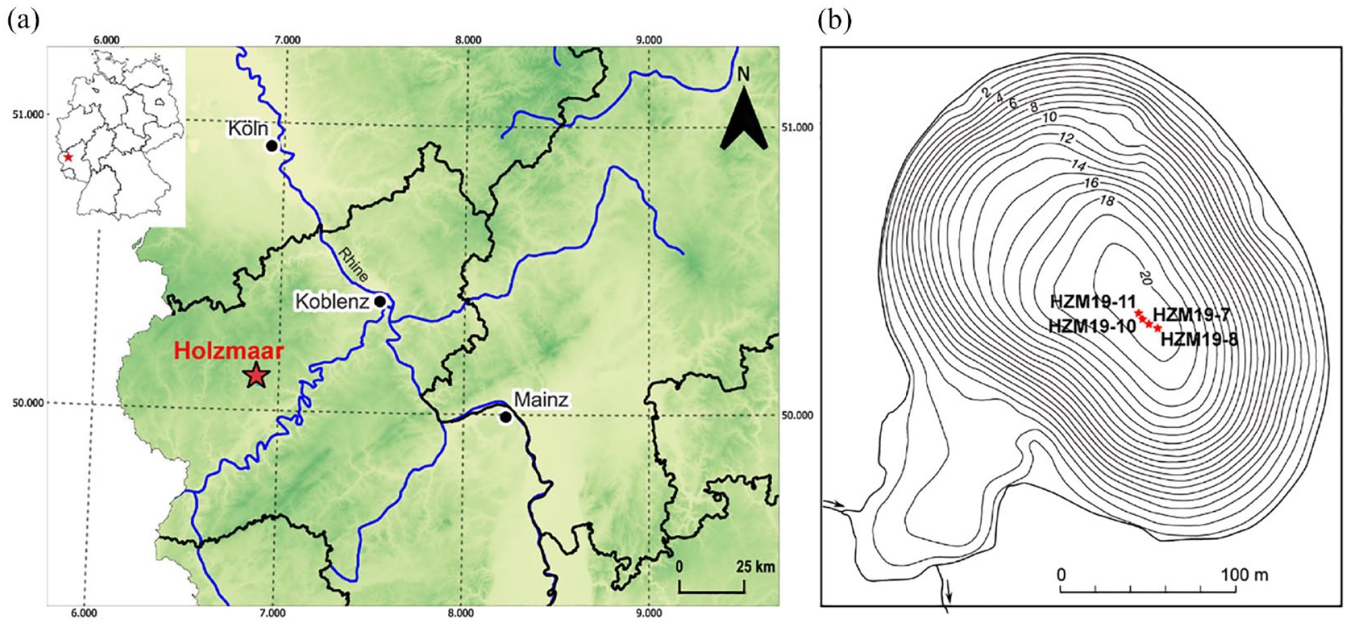
(a) Location of Holzmaar in Germany (upper-left insert) and elevation model of western Germany (NASA/METI/AIST/Japan Space systems and U.S./Japan ASTER Science Team (2019). (b) Bathymetric map with coring sites HZM19-7, 8, 10 and 11 (modified after Zolitschka, 1998 with isobaths in metres relating to the lake level of 1996 CE).

The annually laminated sediments of Holzmaar have been intensively studied since the mid-1980s (e.g. Birlo et al., 2023; Brauer et al., 2001; García et al., 2022b; Negendank and Zolitschka, 1993; Stockhausen and Zolitschka, 1999; Vos et al., 1997; Zolitschka, 1989; Zolitschka et al., 2000; Zolitschka, 1991, 1998). Today, the lake is dimictic (Oehms, 1995), stratifying annually from May until December and may become monomictic in years with ice cover (Lücke, 1998). The hypolimnion is seasonally anoxic (Lücke, 1998) with a maximum thermocline-depth of 6 m (Raubitschek et al., 1999). The trophic status of the modern lake is characterised by a sufficient nutrient availability causing the development of meso- to eutrophic conditions (Scharf and Oehms, 1992). This is supported by studies of diatom assemblages (Hofmann, 1994), submersed macrophyte taxa (Melzer, 1992) and macrozoobenthic communities (Wendling and Scharf, 1992). Additional information about the limnology and geomorphology of Holzmaar is presented elsewhere (Hofmann, 1994; Lücke, 1998; Oehms, 1995; Scharf, 1987). Altogether, the fine-grained varved sediments of Holzmaar recorded environmental and climatic conditions continuously and with high-resolution, ideal for detecting evidences of climate change and anthropogenic impacts through biogeochemical proxies as well as by diatom assemblages.

Coring and chronology

In August 2019, four parallel sediment cores (HZM19-7, HZM19-8, HZM19-10, HZM19-11) were recovered at 18–19 m water depth from the centre of Holzmaar using an UWITEC piston corer from a coring platform (Figure 1b). We use the varve chronology VT22 for dating, which was developed as a segmented and parameter-based integration of varve ages with radiometric dating (Birlo et al., 2022, 2023).

Sediment cores were split in half lengthwise, photographed, and cross correlated macroscopically using a series of distinct marker layers to produce a 15 m long and continuous composite sediment record (HZM19) for further analysis (Birlo et al., 2023).

For this study, we investigated the depth section from 5.65 to 5.1 m composite depth of HZM19. This section is composed of highly organic varves with vivianite (lithozone H8) and of organic varves with clastics (lithozone H9) (Zolitschka et al., 2000) and covers the age range from 2950 to 2450 ± 98 cal. BP. At about 2600 cal. BP (5.43 m composite depth) there is a 1.2 cm thick pale brown minerogenic layer (Figure 2) interrupting the normal sedimentation. This layer is homogeneous and includes fine-grained siliciclastic sediment. Further details on the lithology and chronology of Holzmaar are published elsewhere (Birlo et al., 2022, 2023; Garcia et al., 2022b).

Figure 2.

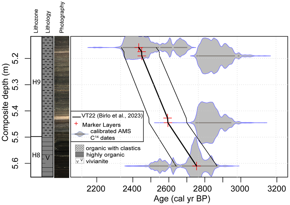
Studied section of the composite profile HZM19 with lithozones, lithology and photography as well as the age-depth model VT22 with marker layers (Birlo et al., 2022, 2023).

Materials and methods

Subsampling

Sediment subsamples for diatom and geochemical analyses were obtained continuously with a 5 ml syringe and a spatial resolution of 1 cm along the time window of the HCA (2950–2450 cal. BP). This subsampling strategy provides a total of 50 samples with, on average, 9 years per sample.

Physical and biogeochemical proxies

Prior to subsampling for destructive analyses, core halves were cleaned and smoothened to apply non-destructive sediment scanning techniques. First, an ITRAX X-ray fluorescence (XRF) core scanner (Cox Analytics) (Croudace et al., 2019; Croudace and Rothwell, 2015) was used to determine the elemental composition with a chromium (Cr) tube and constant settings (30 kV, 50 mA, step size: 0.2 mm, exposure time: 5 s). The output was processed with the software Q-spec (Cox Analytics). Results are expressed in counts (cts) and describe relative intensity variations of 23 elements as well as coherent (coh) and incoherent (inc) scattering. We performed centred log-ratio (clr) transformation of XRF data to normalise the relative changes in element composition to values resembling the chemical sediment composition (Bertrand et al., 2024; Weltje and Tjallingii, 2008). In addition to elemental clr values, we calculate the incoherent/coherent scattering ratio (inc/coh), which is regarded as a proxy for organic matter (OM) content of lacustrine sediments (Woodward and Gadd, 2019). Secondly, magnetic susceptibility (MS) was scanned with 4 mm increments using a Bartington MS2E sensor employed to an automated measuring bench (Nowaczyk, 2002).

Thirdly, hyperspectral image (HSI) scanning was carried out using a Specim PFD-CL-65V10E line-scan camera following the methods of (Butz et al., 2015) with a resolution of 60 μm × 60 μm (pixel size). Relative absorption band depth (RABD) indices were applied to quantify absorption features associated with sedimentary pigments. Details on scanning and index calculations are published by Zander et al. (2021). Two different RABD indices were analysed for this study: the RABD₆₇₁ index represents total chlorophyll (TChl: mainly chlorophyll a, b and coloured transformation products) interpreted as representative of total algal abundance (Butz et al., 2017), while the RABD₈₄₅ index represents bacteriopheophytin a (Bphe a), a specific biomarker for phototrophic purple sulphur bacteria, which live at the chemocline of stratified (meromictic) water bodies indicating that the oxic/anoxic boundary is located in the photic zone of the lake (Sinninghe Damsté and Schouten, 2006). Both indices were calibrated to concentrations (μg.g⁻¹ dry sediment) via linear regression between measurements of extracted sedimentary pigments and average RABD index values of the same sample depths (Birlo et al., 2024). The proxy-proxy calibration (von Gunten et al., 2012) was carried out using an ordinary least square regression (Supplemental Figure S2, available online, Birlo et al., 2024).

Sedimentary pigments were extracted using the combined protocols of Lami et al. (1994) and Pniewski (2020). Pigments from 1 g of wet sediment were extracted by 2 ml of 100% Acetone (HPLC grade), sonication, and maceration over 12 h at −20°C until the supernatant was pale in colour. After a succession of acetone extraction steps, the supernatant with extracted pigments was filtered through a 0.22 mm AFE filter into a 20 ml amber glass vials and stored in dark at −20°C. UV–VIS absorption spectra of pigment extracts were measured with a Shimadzu UV–VIS spectrometer (UV-1800 CE 230 V; 300–800 nm) and a 0.2 nm step size spectral resolution. The concentration of total green pigments (e.g. chlorophyll a and their degradational products such as pheophytins and pheophorbides) was determined based on the absorbance at 666 nm using the Lambert-Beer law and the specific extinction coefficient in an acetone:water (90:10) solution (Jeffrey and Humphrey, 1975) based on the water content of the sediment. Bacteriopheophytin a concentrations were determined similarly using the absorbance at 750 nm and the extinction coefficient according to Fiedor et al. (2002). Furthermore, total green pigments and Bphe a are expressed in μg.g⁻¹ wet sediment using the sample weight and the final volume of the extract.

Prior to destructive geochemical measurements, all subsamples were freeze-dried and homogenised. Total carbon (TC), total nitrogen (TN) and total sulphur (TS) were analysed with a CNS elemental analyser (EuroEA, Eurovector). Total organic carbon (TOC) was measured after acidification (first 3% and then 20% HCl at 80°C) with the CNS elemental analyser, and total inorganic carbon (TIC) was calculated as TC minus TOC. Additionally, the TOC/TN ratio was calculated to distinguish autochthonous from allochthonous sources of organic matter. Low values (<10) are indicative of autochthonous lacustrine productivity (algae), while values >20 are dominated by cellulose of higher plants from allochthonous terrestrial origins (Meyers and Teranes, 2001).

Biogenic silica (BSi) was measured (as SiO₂) by extraction with 1 M NaOH at 85°C for 45 min (Müller and Schneider, 1993). The solution was cycled by a continuous flow system into an auto analyser, where dissolved Si was detected by spectrophotometry. All samples have a BSi content >10 % and a BSi/clay ratio of >0.005. Thus, clay-mineral dissolution during this analysis is not expected (Koning et al., 2002).

Diatom preparation and counting

An aliquot of each of the 50 freeze-dried samples was oxidised with H₂O₂ (30 vol %) and heated in a water bath (~80°C) for 2–5 min to eliminate organic matter (Battarbee, 1986; Battarbee et al., 2001). Samples were then rinsed repeatedly with distilled water until they reached a neutral pH. Permanent slides were mounted using Naphrax. A minimum of 400 valves per slide were counted to calculate relative abundances in percent and numbers of valves per gram of dry sediment according to the modified evaporation try method with square cover slides (Battarbee, 1986). Microscopic observations were made using an Olympus CX40 binocular optical microscope equipped with an immersion objective (Plan Ach 100X/1.25) at the GEOPOLAR lab (University of Bremen) and a Zeiss Axioplan binocular optical microscope equipped with an immersion objective (Plan Neofluar 100X/1.30) with differential interference contrast optics connected to a Gryphax digital camera at the Alfred-Wegener Institute, Bremerhaven. For scanning electron microscope (SEM) observations, aliquots of the cleaned sample were dried on aluminium stubs at room temperature before being coated with gold and examined using a Carl Zeiss SUPRA 40 (5 kV) microscope at the Faculty of Geosciences, University of Bremen.

The floras of Krammer and Lange-Bertalot (1986–1991), Krammer (1997a, 1997b, 2000, 2002), Lange-Bertalot (2001) and Hofmann et al. (2013) were used to identify the diatom taxa. Trophic states of the main taxa were assigned using published data (Van Dam et al., 1994). Specialised taxonomic publications were considered to support the identification and ecology of some diatom genera such as Stephanodiscus, Lindavia, Pantocsekiella (Ács et al., 2016; Håkansson, 1986; Häkansson, 2002; Häkansson and Kling, 1989; Nakov et al., 2015) and Fragilaria (Crawford et al., 1985; Saros et al., 2005).

Statistical analyses

Principal component analysis (PCA) was performed for diatom species as a basis for visually grouping observations. Stratigraphic zones of similar diatom assemblages were delineated using stratigraphically constrained incremental sum of squares (CONISS) cluster analysis (Grimm, 1987). Only diatom species with a relative abundance >5 % in at least two samples were considered. Prior to any statistical analyses (both PCA and clustering), we have transformed the relative abundance applying the Hellinger method (Legendre and Gallagher, 2001). The number of significant clusters (i.e. diatom zones) was determined by comparison with the broken stick model (Borcard et al., 2011). All analyses were performed in R version 4.1.1 (R Core Team, 2021) using the vegan (Oksanen et al., 2022) and rioja packages (Juggins, 2022a). The package RiojaPlot was used for stratigraphic plots (Juggins, 2022b).

Generalised additive models (GAMs) were fitted to selected biogeochemical variables and trends in the data were identified using mgcv v.1.8–42 (Wood, 2017; Wood et al., 2016; Wood, 2023) and gratia v.0.8.1.26 (Simpson, 2023) packages in R. GAMs are a regression-based method for estimating trends that use a sum of smooth functions to model nonlinear relationships between covariates and their response (Simpsona and Anderson, 2009). Models were fitted using penalised residual maximum-likelihood, in which a penalty controls the degree of ‘wigglyness’ of estimated trends with an adaptive smoother (Wood, 2011). We use a Gaussian model for BSi, TChl and Bphe a and the tweedie model for Ti. Identification of periods with significant environmental change was realised using the first derivative of estimated trends, which are identified for those times where the simultaneous confidence interval of the first derivative moved away from zero. See Simpson (2018) for further details about the GAMs modelling approach.

Results

Physical and geochemical proxies

Selected proxies from the physical and geochemical analyses are presented in Figure 3 (extended version as Supplemental Figure S3, available online). All data sets are available online (García et al., 2024a, 2024b, 2024c, 2024d, 2024e, 2024f). Between 2950 and 2450 cal. BP, MS shows a slight increase from bottom to top with a maximum around 2600 cal. BP (Figure 3). We use Ti as an indicator of allochthonous siliciclastic input (cf., García et al., 2022a, 2022b). Ti has lowest values between 2750 and 2670 cal. BP and the highest value occurs at ca. 2600 cal. BP.

Figure 3.

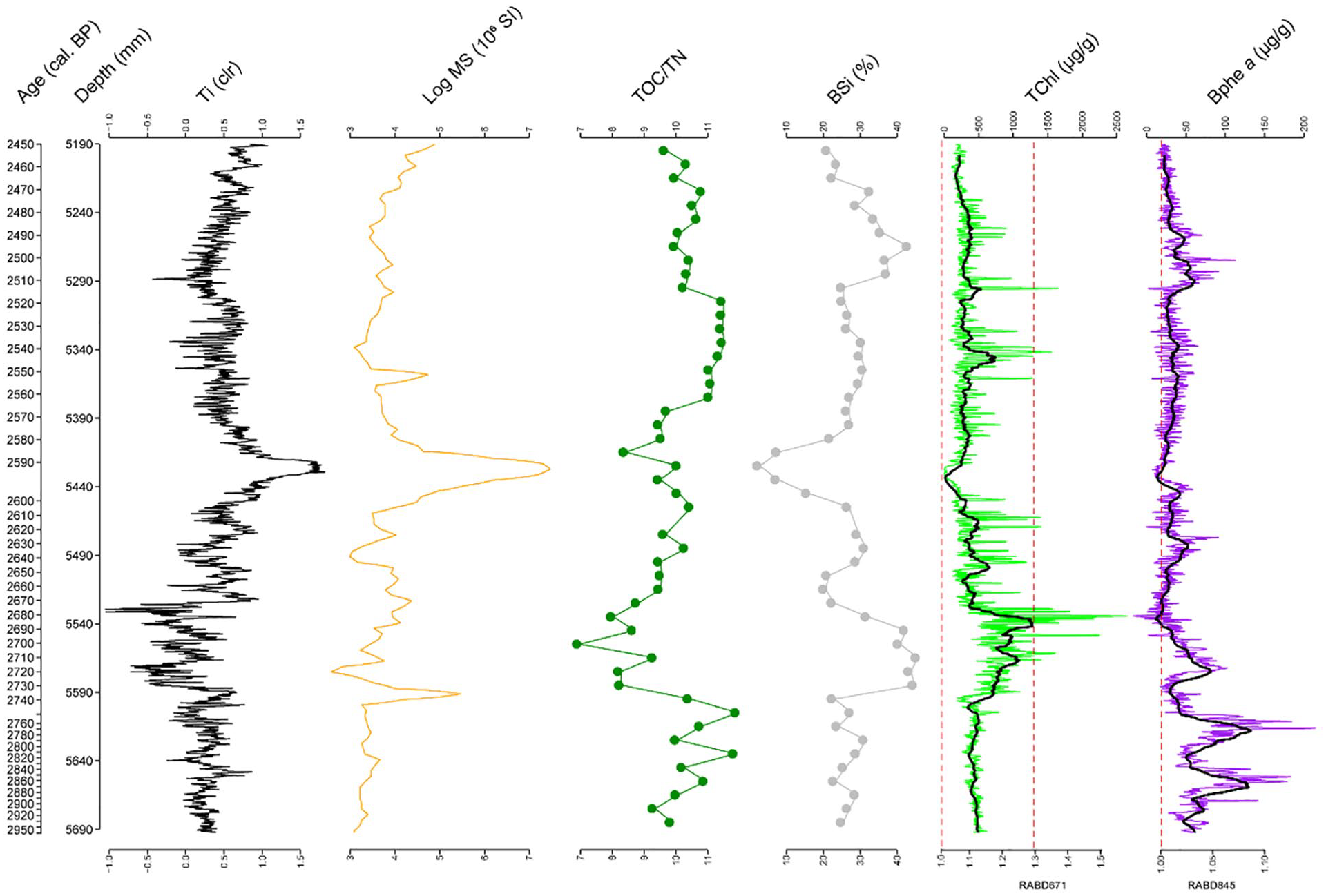
Selected biogeochemical proxies for the Homerian Climate Anomaly: titanium (Ti), magnetic susceptibility (MS), TOC/TN ratio, biogenic silica (BSi), HSI index and sedimentary pigment concentration of total chlorophyll (TChl) and bacteriopheophytin a (Bphe a), black lines are 100-pt. moving averages).

The TOC/TN ratio increases to a maximum at 2750 cal. BP from where it decreases towards ca. 2700 cal. BP; from then onwards, it shows an increasing trend again. BSi displays maximum values between ca. 2730 and ca. 2680 cal. BP and intermediate to low values from 2700 to 2600 cal. BP with a minimum at 2600 cal. BP from where it increases to intermediate and high values until the top of our record.

The HSI records show a maximum of TChl between 2740 and 2680 cal. BP and a minimum around 2600 cal. BP; Bphe a presents higher values before 2750 cal. BP (two maxima at ca. 2760 and 2850 cal. BP), a smaller peak at ca. 2700 cal. BP and subsequently decreases significantly and remains almost absent towards the top.

Around 2600 cal. BP, we observe an event layer (Figure 2, Supplemental Figure S3, available online) with responses recorded by almost all proxies: Ti and MS increase to maximum values, while organic parameters such as BSi, TOC/TN, and all measured pigments decrease to minima (Figure 3, Supplemental Figure S3, available online).

The fitted GAMs for Ti, BSi, TChl and Bphe a explain more than 76% of the total deviance for each model (Supplemental Table S1 and Figure S1, available online). Thus, the discrepancy between observations and fitted values is low. First derivatives of the fitted trends for all variables indicate one significant period of change from 2750 to 2700 cal. BP (Figure 4). Before 2750 cal. BP, Ti presents some minor and short-lived local maxima, which could be related to increased run-off. However, this is not supported by MS values. Bphe a also has large variability with some local maxima suggesting extended – if not permanent – anoxia. Ti, BSi and TChl have significant changes around 2600 cal. BP (Ti maximum, BSi and TChl minima, cf. Figure 3, Supplemental Figure S3, available online). These are related to the event layer at this depth. Afterwards all variables present short periods of change until the top of our record.

Figure 4.

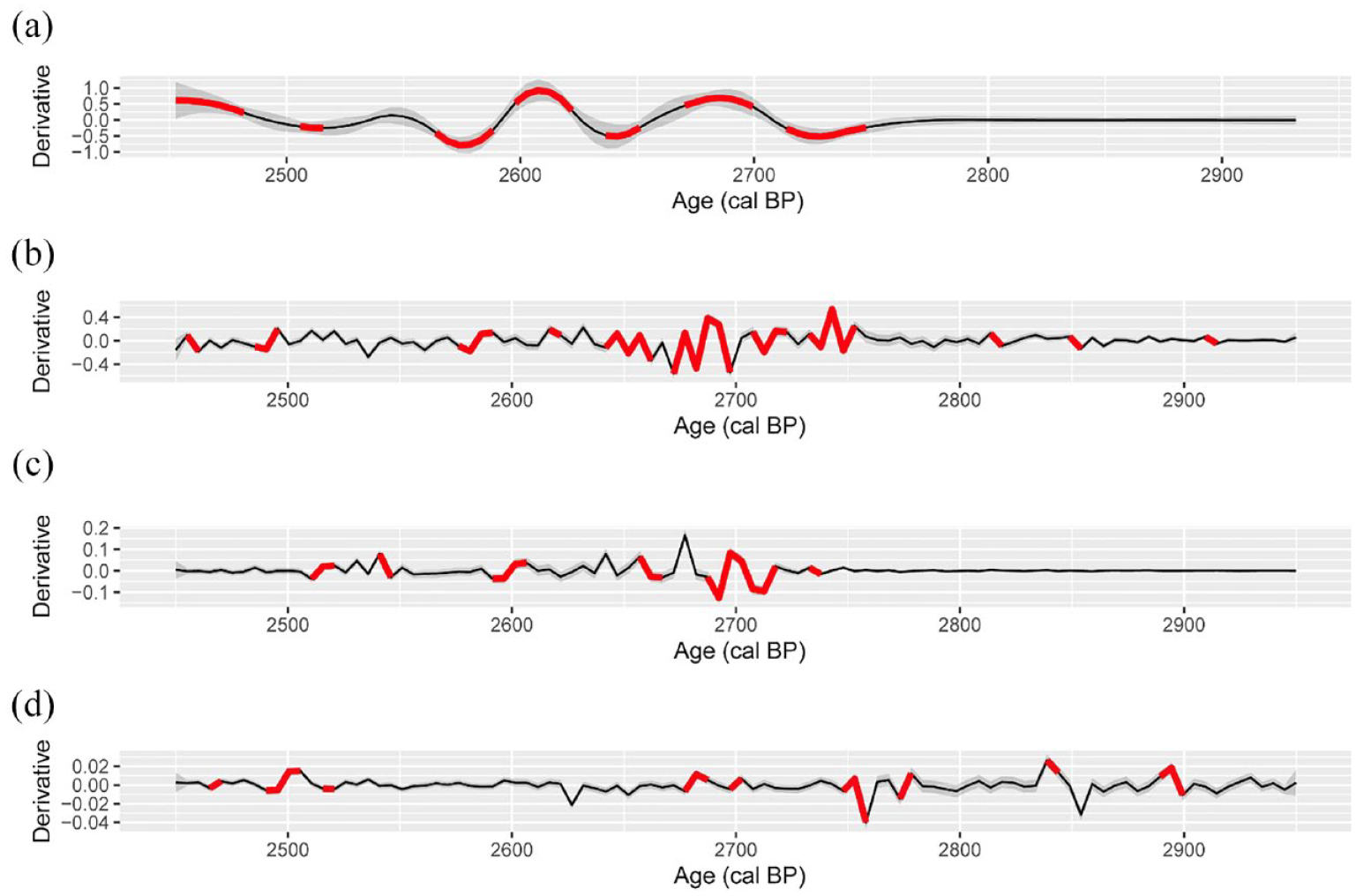
First derivatives of fitted GAMs for (a) biogenic silica (BSi), (b) titanium (Ti), (c) total chlorophyll (TChl) and (d) bacteriopheophytin a (Bphe a) versus age (VT22). Thick red lines identify periods of significant change for each variable, grey areas represent 95% confidence intervals.

Diatom stratigraphy

A total of 89 taxa within 49 genera have been identified for the studied time window (2950–2450 cal. BP). The data set is available online (García et al., 2024g). Only nine taxa are presented with >5% (diatom values are given in relative abundances) in at least two samples. Of these taxa, seven are planktonic and three are benthic species. The total abundance of diatoms is supported by measurements of BSi. The diatom stratigraphy (Figure 5, Supplemental Figure S6, available online) is divided into four statistically significant diatom zones (DZ) based on the broken stick model (Supplemental Figure S7, available online) with one of them being divided into two subzones. Moreover, to detect patterns of diatom assemblages we performed a PCA on the data set (Supplemental Figure S5, available online) that is also coloured to distinguish between the DZs (Supplemental Figure S5, available online).

Figure 5.

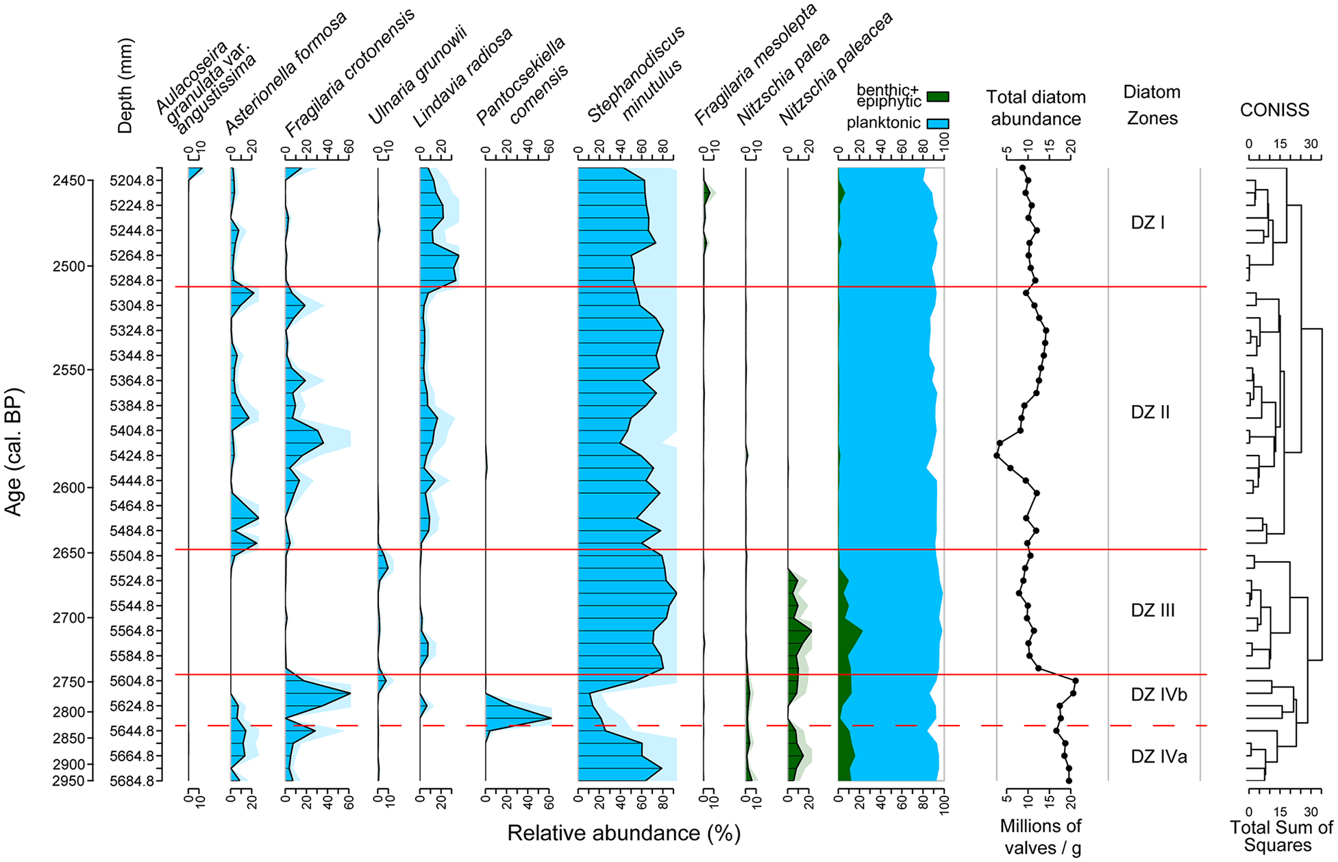
Diatom stratigraphy of HZM19 versus time for the studied period with the CONISS cluster analysis results to the right. Only taxa with a relative abundance >5% in at least two samples are shown. Taxa are divided into planktonic (blue) as well as into epiphytic and benthic diatoms (green). Diatom total abundance is shown as millions of valves/g of dry sediment. Exaggerated curves are shaded in light blue and light green. Red horizontal lines indicate the diatom zones according to CONISS, the dashed red line marks the diatom subzone.

DZ IV (2950–2750 cal. BP) consists of two subzones with the subdivision based on variations of Stephanodiscus minutulus. The lower DZ IVa (2950–2860 cal. BP) shows mid to low values of total diatom abundance and the dominant species is planktonic S. minutulus (60%–80%). The benthic species Nitzschia paleacea and N. palea appear in low percentages (<20%), as well as planktonic Asterionella formosa and Fragilaria crotonensis (ca. 20%). The upper DZ IVb (2860–2750 cal. BP) has a similar total diatom abundance. However, there is a marked decrease in S. minutulus to ca. 10%–20% and benthic species almost disappear. The two dominant planktonic species are now Pantocsekiella comensis and Fragilaria crotonensis (ca. 50%–60%). Lindavia radiosa and Ulnaria grunowii are present with very low values (5%–10%). Benthic species partially disappear and reappear at ca. 2760 cal. BP.

DZ III (2750–2650 cal. BP) shows an increase of total diatom abundance. Pantocsekiella comensis and Fragilaria crotonensis disappear completely during DZ III. Lindavia radiosa and Ulnaria grunowii remain present only with low values (ca. 5%–10%). Stephanodiscus minutulus reappears and becomes the dominant species with highest values of the record (80%–90%). The benthic species Nitzschia paleacea and N. palea also reappear with slightly higher values than before and a small peak shortly before 2700 cal. BP (20%).

During DZ II (2650–2510 cal. BP), the total diatom abundance has similar average values like for DZ III although with a minimum at ca. 2600 cal. BP. Stephanodiscus minutulus remains dominant during this zone but with slightly lower percentages than in DZ III. Asterionella formosa and Fragilaria crotonensis reappear with values between 20% and 40%. Lindavia radiosa remains present with slightly higher percentages (ca. 20%), while Ulnaria grunowii and benthic species disappear completely.

Finally, during DZ I (2510–2450 cal. BP) the total diatom abundance decreases compared to DZ II. Stephanodiscus minutulus remains dominant but with lower percentages. Asterionella formosa and Fragilaria crotonensis are present but with very low values (<10%). There is a marked increase in percentages of Lindavia radiosa reaching 30%. The benthic species Fragilaria mesolepta and the planktonic Aulacoseira granulata var. angustissima appear for the first time with very low values (<10%).

Paleoenvironmental interpretation

Variations in diatom assemblages, physical and geochemical proxies during the studied time window (2950–2450 cal. BP) are related to explanatory climatic and anthropogenic forcing factors. To streamline our interpretation, we label the TSI-defined time window of 2750–2680 cal. BP as full HCA, the two centuries prior to the HCA as pre-HCA (2950–2750 cal. BP) and the 230 years after the HCA as post-HCA (2680–2450 cal. BP). These three periods almost coincide with the most prominent changes in the diatom record characterised by their respective diatom zones: 2950–2750 cal. BP (DZ IV), 2750–2650 cal. BP (DZ III) and 2650–2450 cal. BP (DZ I and II).

The pre-HCA (2950–2750 cal. BP, DZ IV)

This period is divided into two diatom subzones (Figure 5), which are closely link and unrelated to the rest of the diatom record (Supplemental Figure S5, available online). Both subzones are interpreted as a transition from a more eutrophic state with dominance of S. minutulus (DZ IVa, 2950–2825 cal. BP) to a mesotrophic state (DZ IVb, 2825–2750 cal. BP) with strong thermal stratification and dominance of Pantocsekiella comensis and Fragilaria crotonensis. We previously interpreted S. minutulus as being associated with higher nutrient availability and a well-mixed water column (weak thermal stability), whereas Pantocsekiella comensis and Fragilaria crotonensis both tend to form chain colonies suggesting strong thermal stratification. As these species need more resistance against sinking to remain in the photic zone, they require less mixing of the water column (García et al., 2022b; Jaworski et al., 1988; Padisák et al., 2003). Additionally, there are two peaks of Bphe a (Figure 3) at 2860 cal. BP (last part of DZ IVa) and at 2760 cal. BP (last part of DZ IV b) that can be related to anoxic events supporting our hypothesis. These peaks are also linked to minor maxima of the benthic species N. paleacea (Figure 5). This eutrophic taxon, which may be related to higher summer temperatures and possibly less wind-stimulated mixing, is also compatible with the hypothesised anoxia (Baier et al., 2004). An increasing trend of the TOC/TN ratio during DZ IV is indicative of aquatic organic matter with higher proportions of macrophytes, which increases the N input to the lake system and, as a consequence, is beneficial for the development of Fragilaria crotonensis.

The HCA (2750–2680 cal. BP, DZ III)

There are nutrient-rich conditions with weak thermal stratification, possibly related to windier conditions (Moreno-Ostos et al., 2009; Reynolds, 1993), which are supported by dominance of S. minutulus. The presence of Ulnaria grunowii also supports a weaker thermal stratification. Even though the latter species is another species from the ‘thin and long Fragilaria/Ulnaria group’, it requires different ecological conditions than Fragilaria crotonensis because it does not form colonies and is more silicified. Thus, it needs more turbulence to remain in the photic zone. A well-mixed water column is also supported by a peak in TChl, possibly due to blooms of S. minutulus. The decreasing TOC/TN ratio is suggesting a more autochthonous source of organic matter, that is, higher lacustrine productivity. Furthermore, Bphe a disappears almost completely after 2750 cal. BP, except for a small and short anoxic event around 2700 cal. BP, also reflecting well-mixed conditions. Furthermore, this is supported by the most distinct periods of ecosystem change documented by the first derivative of GAMs around 2750 cal. BP (Figure 4).

As an indicator for solar forcing variability we use the ¹⁴C production rate of the IntCal20 calibration curve (Harding et al., 2023; Reimer, 2020; Muscheler et al., 2014) and total solar irradiance (TSI) (Steinhilber et al., 2009). Both records are proportionally inverse (Kromer et al., 2001). The ¹⁴C production rate and TSI show high values for the period 2750–2680 cal. BP, that is, for the HCA (Figure 6). Changes of diatom assemblages and biogeochemical proxies during DZ III are in phase with the HCA and support the signature of this climate anomaly between 2749 and 2680 ± 98 cal. BP (DZ 3, Figures 5 and 6).

Figure 6.

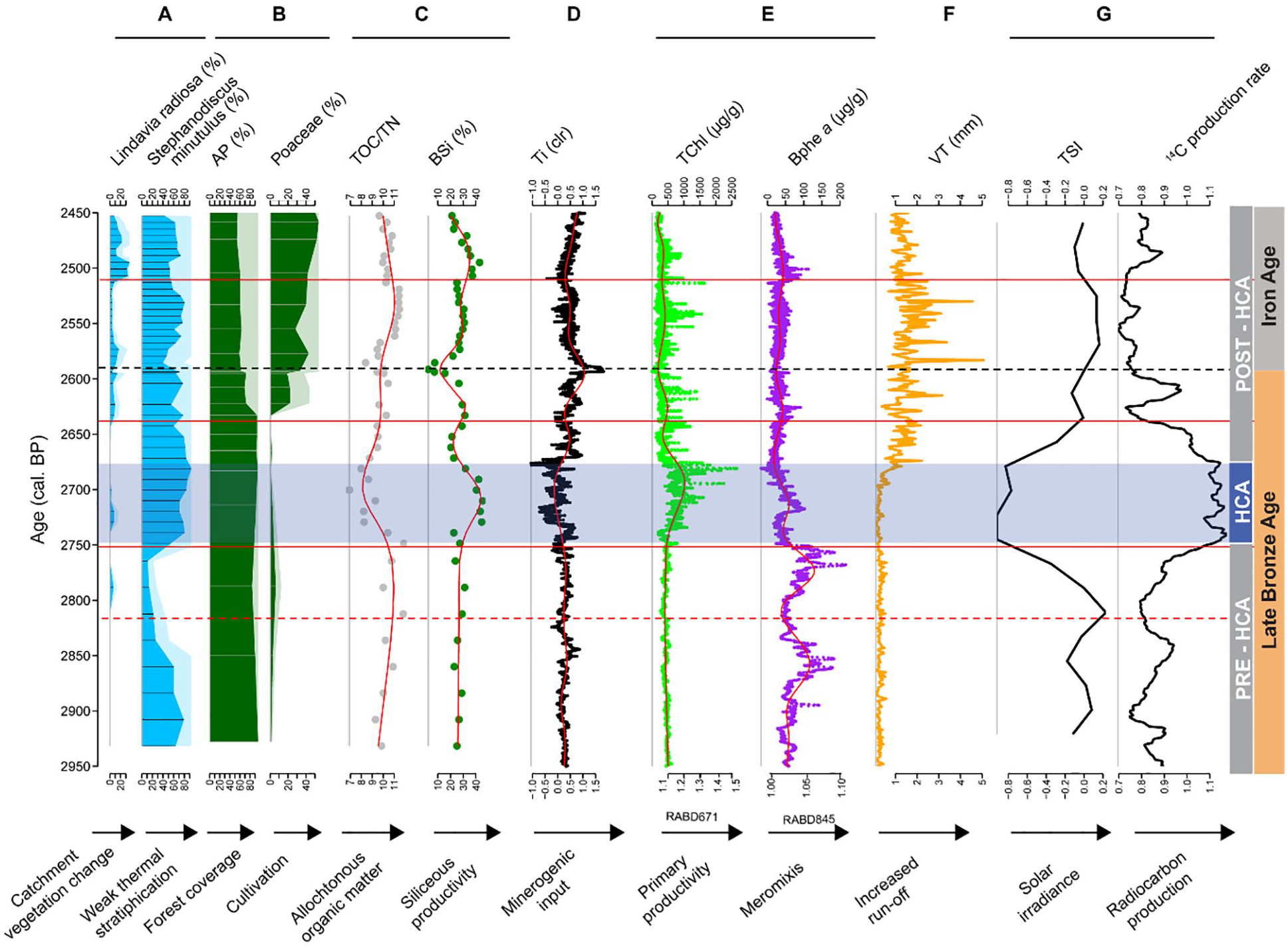
Summary of relevant proxies for the Homerian Climate Anomaly (HCA) at Holzmaar with environmental and climatic interpretations. (a) Key diatom species, (b) Arboreal pollen (AP) and Poaceae (Usinger and Wolf, unpublished data), (c) proxies for allochthonous organic matter (TOC/TN) and autochthonous lacustrine productivity (BSi), (d) Titanium (Ti) as proxy for minerogenic input or soil erosion, (e) HSI record for lacustrine productivity (TChl) and anoxic conditions (Bphe a), (f) varve thickness (VT) (Zolitschka et al., 2000), (g) total solar irradiance (TSI) (Steinhilber et al., 2009) and radiocarbon production rate as proxies of solar activity (Muscheler et al., 2014; Reimer, 2020). Blue shading delimits the HCA based on the TSI data, the black dotted line separates the Late Bronze Age from the Iron Age (Litt et al., 2009), and red horizontal lines indicate diatom (sub)zones boundaries (cf., Figure 5).

Even though the climatic mechanisms controlling the HCA environmental variability are only vaguely understood, there is evidence for colder conditions in Central Europe (Affolter et al., 2019; Wanner et al., 2011, 2015). Some proxies document a climatic deterioration at 2600 cal. BP: speleothems in Spain (Cruz et al., 2015) and peatlands in Ireland (Swindles et al., 2007). However, high-resolution investigation of varved lake sediments from Meerfelder Maar (West Eifel Volcanic Field, Germany), provides insights into atmospheric circulation patterns. These patterns shifted abruptly and in phase with the HCA documenting an increase of windiness as recorded by Stephanodiscus sp. blooms and wind-sensitive varve thickness variations between 2759 ± 39 and 2560 ± 48 cal. BP. These responses were caused by slightly cooler conditions and an increase in precipitation (Harding et al., 2023; Martin-Puertas et al., 2012). The dominance of Stephanodiscus spp. in both Meerfelder Maar and Holzmaar can thus be linked to colder conditions. As diatom assemblages are not a direct proxy to estimate temperature changes of the past, they might be influenced by temperature-dependant catchment weathering causing changes in lake-water chemistry. Together, this is reflected in their ecological ranges and thus in diatom assemblages (Anderson, 2000; Sommaruga-Wögrath et al., 1997). Stronger winds during the HCA were also reported from Diss Mere, England (Harding et al., 2023) between 2767 ± 29 and 2638 ± 28 cal. BP. While observations of diatom blooms for Meerfelder Maar are based on microfacies analysis of thin section, for Diss Mere detailed diatom studies were carried out supporting windy (stormy) conditions during the HCA (Harding et al., 2023).

Durations of the HCA obtained for the three compared varved lakes are different (Meerfelder Maar: 199 ± 9 years, Diss Mere: 149 ± 8 years (both (Harding et al., 2023) and Holzmaar: 69 ± 4 years. Considering the uncertainties of all three applied age-depth models, the duration of the HCA at Holzmaar overlaps with the age ranges considered for both Meerfelder Maar and Diss Mere supporting the regional response to solar forcing. Despite of this, defining the response of a lacustrine system to an event such as the HCA is always problematic since their impacts probably are regionally very different.

The post-HCA (2680–2450 cal. BP, DZ II and I)

The changes that occurred after 2680 cal. BP seem to be the end of the climate deterioration. But also the start of significant cultural change at the transition from the Late Bronze Age to the Iron Age around 2600 cal. BP (Litt et al., 2009). The varve thickness increase observed at Holzmaar (Figure 6, Zolitschka et al., 2000) seems unrelated to the diatom response for the HCA at 2750 cal. BP. Varve thicknesses at Holzmaar start to increase at 2680 cal. BP, which is after the on-set of the HCA and seems to be linked to deforestation as shown by pollen data and later on by diatoms (Figure 6). We cannot relate the varve thickness variability to the HCA signal and link it to wind intensity as proposed for Meerfelder Maar (Martin-Puertas et al., 2012), as Holzmaar was protected by a forest (Figure 6) until 2680 cal. BP. Furthermore, Ti increases after 2680 cal. BP and also indicates increased run-off. Moreover, varve thickness of Holzmaar does not decrease after the HCA as reported for Meerfelder Maar but maintains higher levels, which suggests subsequent changes in the catchment due to anthropogenic impacts, evidenced by the increase of non-arboreal pollen and L. radiosa, that is, increased soil erosion with higher nutrient influx due to agricultural activities, which resulted in higher lacustrine productivity.

From 2650 cal. BP onwards we observe changes in diatom assemblages (Fragilaria crotonenesis, Asterionella formosa and Lindavia radiosa reappear) and increases in TOC/TN, Ti and MS. At this time, late Bronze Age settlements were regionally abandoned, and early Iron Age cultures and technologies started to spread, which coincides with numerous archaeological findings (e.g. Dörfler et al., 1998). The beginning of the Iron Age as defined by Litt et al. (2009) is recognisable in our record by a minerogenic layer (Figure 1 at 5.43 m). This event layer is characterised by peaks in Ti and MS at ca. 2600 cal. BP and probably related to deforestation-enforced higher run-off. Even though this seems to be a local event, there is evidence from other sites, which supports increased run-off and vegetation changes during this period (Dabkowski et al., 2015; Schittek et al., 2021; Zander et al., 2023). During the last period of post-HCA, DZ I (2510-2450 cal. BP), there is a further increase in Ti and MS which is followed by a distinct increase of L. radiosa. This species is related to changes in catchment vegetation (Bitušík et al., 2018; Hickman and Reasoner, 1998) and correlates to increasing non-arboreal pollen in response to intensified forest clearing (Litt et al., 2009, Usinger and Wolf, unpublished data).

According to changes in the ¹⁴C production rate (Muscheler et al., 2014; Reimer, 2020), a secondary solar minimum with a lower amplitude than the HCA occurs from 2625 to 2575 cal. BP with probably less impact on atmospheric processes. For the annually laminated record from Diss Mere, Harding et al. (2023) did not recognise this secondary solar minimum although it was observed for Meerfelder Maar using varve thickness as a wind-proxy (Martin-Puertas et al., 2012). The authors conclude that Diss Mere was not sensitive to this lower amplitude solar forcing because sea-level air pressure centres affected the regional impact of mainly north-easterly circulation at that time (Harding et al., 2023). Such a difference between Diss Mere and Meerfelder Maar seems reasonable because Diss Mere is strongly influenced by climate forcing of the East Atlantic pattern (Sjolte et al., 2018), which is less correlated with long-term solar forcing.

For Holzmaar, a signal of this second solar minimum was also not observed. If present at all, this solar signal is mixed with or overwritten by anthropogenic impacts at the start of the Iron Age. This is supported by a significant change of the pollen record for Holzmaar (Figure 6, Usinger and Wolf, unpublished data), which is also documented by Litt et al. (2009) showing a transition from beech (Fagus) forest to dominance of an open landscape with Poaceae for Meerfelder Maar and Holzmaar. At Holzmaar this is also recorded by diatom assemblages, as increasing L. radiosa indicates changes in catchment vegetation. Assuming a similar climatic forcing for the neighbouring lakes of Meerfelder Maar and Holzmaar, the difference regarding the second minor solar minimum needs to be explained by local factors, that is, influences from the catchment area on the respective lacustrine systems.

In this respect, Meerfelder Maar has a water-surface almost 10x larger with a catchment area almost 3x as large as Holzmaar. However, the ratio between catchment and lake-surface area, an indicator for the potential level of catchment influences on a lacustrine system, is 3x higher for Holzmaar (34.5) compared to Meerfelder Maar (11.5). Therefore, changes in the catchment area are supposed to have a much higher influence on the lake system of Holzmaar. In addition, the crater slopes at Meerfelder Maar reach an elevation of nearly 200 m above lake level, while this elevation difference is only 52 m for Holzmaar providing much less wind protection. In combination, Holzmaar is more sensitive to catchment-related changes, most of all deforestation, which overprints the secondary and lower amplitude solar minimum detected by ¹⁴C production rates (Muscheler et al., 2014; Reimer, 2020).

Conclusions

With this high-resolution multiproxy investigation, we document the responses of the lake system at Holzmaar to one of the most important GSM of the Holocene – the Homerian Climate Anomaly (HCA). We analysed diatom assemblages and physical as well as biogeochemical proxies from varved sediments of Holzmaar to determine if this lake system responded to the HCA and whether it is possible to differentiate between lake responses to climatic and to anthropogenic influences.

We conclude that from 2950 to 2750 cal. BP the responses of the lake system are related to anoxia with maxima around 2860 cal. BP and 2760 cal. BP together with strong thermal stratification. We call this period the pre-HCA scenario. From 2750 to 2680 cal. BP, all proxies changed and indicate colder, more humid and windier conditions, which relate to HCA. The final period from 2680 to 2450 cal. BP marks the ending climate deterioration mixed with evidences of human impact. Anthropogenic influences intensify towards 2600 cal. BP, when diatom assemblages and pollen data indicate forest clearance in the catchment area, a period we call the post-HCA scenario. Similarities between HCA and the pre-HCA scenarios are questionable with regard to diatom assemblages (Figure 6). However, differences shown by the species PCA (Supplemental Figure S5, available online) and knowing that there are differences for other proxies such as Ti and Bphe a, evidences that these two periods belong to different scenarios.

Based on this and other studies, the end of the HCA is unclear and debatable. In accordance with the ¹⁴C production rate, it can be defined to 2575 cal. BP (including the second peak), while with the TSI (lower resolution than ¹⁴C production rate), 2680 cal. BP is more realistic. Moreover, proxy evidences recovered from several sites differ. Even when comparing close by sites, like Holzmaar and Meerfelder Maar, there are dissimilarities as local influences on these small lake basins have larger effects and overwrite regional climate signal.

Our study emphasises the importance of high-resolution analyses for a time window that involves both, short and event-like climate signals as well as anthropogenic influence. Even though we did not manage to disentangle both signatures with the studied proxies with certainty, we provide evidence for the HCA and help to better understand the regional responses to this GSM. We also address the different responses to this event by comparing the varved Holzmaar record with the study of two other varved sites – Meerfelder Maar and Diss Mere.

Building on the topic of this investigation, our current project uses the excellent time control provided by the varved lake record from Holzmaar and others available from different parts of Central Europe. It is our future aim to extend the available multiproxy but local dataset from Holzmaar by capturing regional environmental variability in relation to the unique climatic episode of the HCA by investigating other varved records from Central Europe with a similar analytical approach.

Supplemental Material

sj-docx-1-hol-10.1177_09596836241275008 – Supplemental material for Ecological responses to solar forcing during the Homerian Climate Anomaly recorded by varved sediments from Holzmaar, Germany

Supplemental material, sj-docx-1-hol-10.1177_09596836241275008 for Ecological responses to solar forcing during the Homerian Climate Anomaly recorded by varved sediments from Holzmaar, Germany by María Luján García, Stella Birlo, Petra Zahajská, Giulia Wienhues, Martin Grosjean and Bernd Zolitschka in The Holocene