Sage Journals: Discover world-class research

Abstract

In high northern latitudes, the Middle to Late-Holocene was a time of orbitally-induced atmospheric cooling. This led to increased sea-ice production in the Arctic Ocean and its export southward, a decrease in sea surface temperatures (SST), and glacier advances at least since 5–4 ka BP. However, the response of the ocean-climate system to decreasing insolation was not uniform. Our research shows that the sea-ice cover in the northwestern Barents Sea experienced a late response to Neoglacial cooling. We analyzed dinoflagellate cyst assemblages from a sediment core from Storfjordrenna, south of Svalbard. We found that the area experienced ice-free conditions throughout most of the Mid- and Late-Holocene. It was only after 2.3 ka BP that the study site became covered with winter drift ice and primary productivity decreased subsequently. Other regional data support the decrease in SST, the expansion of the sea-ice cover, and the deterioration of the environmental conditions around that time. Our findings indicate that the sea-ice cover in the northwestern Barents Sea required a significant amount of time to respond to the general cooling trend in the region. These results have important implications for present-day environmental changes. Even if the current warming trend is revoked in the future, the observed sea-ice loss in the Barents Sea may be incredibly challenging to reverse.

Keywords

dinoflagellate cysts Echinidinium karaense Islandinium minutum Late-Holocene Operculodinium centrocarpum s.l.PIP25 Storfjordrenna Svalbard XRF

Introduction

The Middle to Late-Holocene in high northern latitudes was a time of decreasing temperatures (McKay et al., 2018) caused by declining boreal summer insolation (Laskar et al., 2004) and referred to as Neoglacial cooling (Wanner, 2021). Around 5 ka BP the modern sea level was reached and the postglacial flooding of the Laptev Sea shelves was finalized (Bauch et al., 2001), allowing the Arctic sea-ice production, which predominantly takes place on the shallow Arctic shelf areas, to reach its modern magnitude (Werner et al., 2013). This resulted in the onset of modern-like conditions with perennial sea ice in the Arctic Ocean (Cronin et al., 2010). Enhanced Mid-Holocene Siberian river runoff caused an eastward shift of Transpolar Drift and increased sea-ice export through the Fram Strait (Dyke et al., 1997; Prange and Lohmann, 2003). Data from the Greenland Ice Core Project ice core show the onset of atmospheric cooling between 5 and 4 ka BP (Dahl-Jensen et al., 1998). Although in the northern North Atlantic region there is no compelling evidence for any significant and widespread climatic anomaly (Bradley and Bakke, 2019) associated with the 4.2 ka BP event (Renssen, 2022) that marks the onset of the Late-Holocene (Walker et al., 2019), a compilation of glacier records indicates a significant climatic transition referred to as “the Holocene Turnover” occurred ~4 ka BP. It represents a dynamical adjustment that subsequently resulted in the establishment of a new climate regime or mode rather than being a multidecadal or centennial deviation from mean conditions (Paasche et al., 2004; Paasche and Bakke, 2009). On Svalbard, Late-Holocene glacier re-advances started around 4 ka BP (Farnsworth et al., 2020). Tidewater glaciers, which were largely absent in Svalbard during the early and Mid-Holocene, reappeared 3–4 ka BP (Jang et al., 2023; Svendsen and Mangerud, 1997). Similarly, in northern Norway, glaciers reappeared ~4 ka BP (Bakke et al., 2005). This coincides with the onset of sea surface temperature (SST) decrease in the northwestern Barents Sea continental slope (Rigual-Hernández et al., 2017; Risebrobakken et al., 2010). In the subpolar North Atlantic, pronounced SST cooling was observed between 4 and 2 ka BP (Orme et al., 2018). A significant sea-ice advance accompanied by distinct sea-ice fluctuations occurred in the eastern Fram Strait after 3 ka BP (Müller et al., 2012). By 2 ka BP, the SST in the Norwegian Sea had already decreased to its Holocene low (Andersen et al., 2004). However, the response of the ocean environment to decreasing boreal summer insolation was not uniform (Andersen et al., 2004, 2004; Wanner, 2021). Around 2 ka BP, the North Atlantic Oscillation, the dominant mode of atmospheric variability at mid-latitudes in the North Atlantic region, changed from variable, intermittently negative to generally positive conditions (Olsen et al., 2012), indicating stronger westerlies. This caused increased Atlantic Water (AW) advection into the Nordic Seas (e.g. Giraudeau et al., 2010; Spielhagen et al., 2011; Telesiński et al., 2014, 2015; Werner et al., 2013). As a result, ocean (e.g. Andersen et al., 2004; Sarnthein et al., 2003), as well as atmospheric (e.g. Johnsen et al., 2001; McDermott et al., 2001) warming, occurred. In Europe and the North Atlantic region, it is recognized as the Roman Warm Period (e.g. Bianchi and McCave, 1999; Matul et al., 2018; Wang et al., 2012).

Here we reconstruct paleoenvironmental changes in the northwestern Barents Sea during the Late-Holocene to estimate how fast the sea-ice cover reacted to changes in the atmosphere and the ocean. We analyze proxy data from a marine sediment core from Storfjordrenna, south of Svalbard, including dinoflagellate cyst (dinocyst) assemblages, as well as previously published XRF data, stable isotope, and alkenone-based SST records. Based on the abundance of indicator species of dinocysts, we reconstruct the reappearance of winter drift ice, as well as the changing influence of AW on the study site. We also compare our data with biomarker-based reconstruction of sea ice from a core from the Olga Basin, northern Barents Sea (Berben et al., 2017).

Oceanographic setting

The Barents Sea is an Arctic shelf sea between the Nansen Basin of the Arctic Ocean to the north, Novaya Zemlya to the east, Scandinavia to the south, the Norwegian Sea to the west, and the Svalbard archipelago to the north-west (Figure 1). The Barents Sea is influenced by several water masses. For this reason, strong environmental gradients can be observed here, making it a great area for studying paleoceanographic changes (e.g. Berben et al., 2017; Knies et al., 2017; Łącka et al., 2015, 2019).

Figure 1.

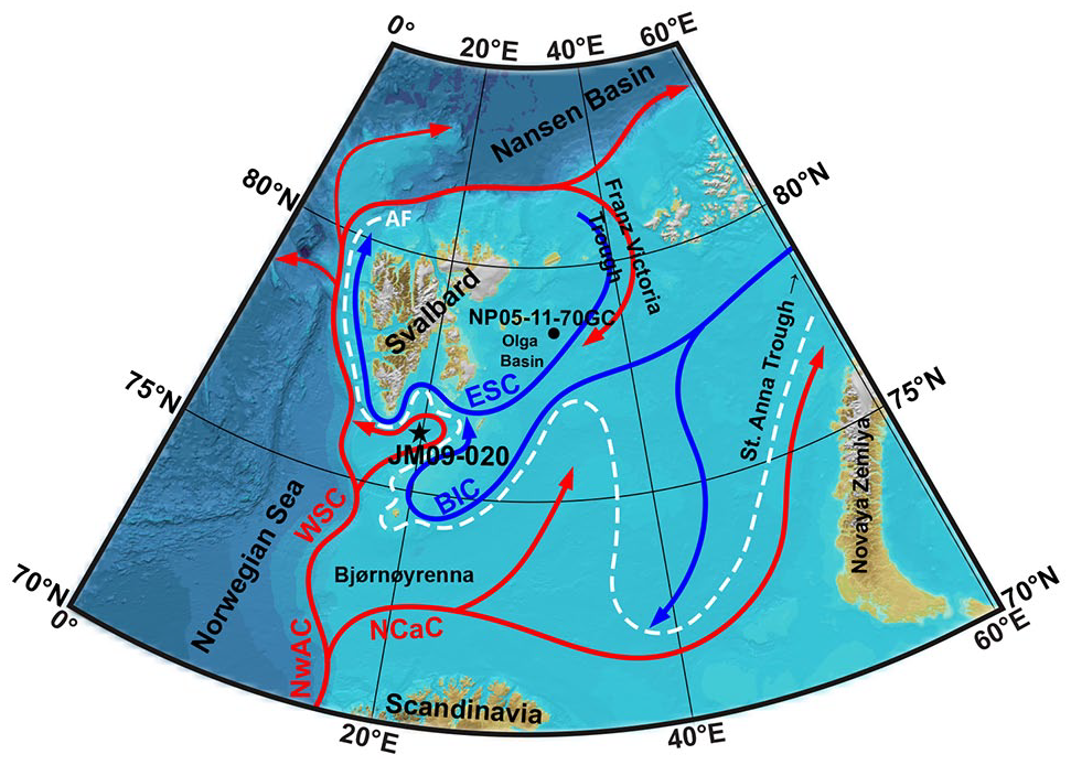
Schematic map showing present-day surface water circulation in the Barents Sea. Red arrows indicate Atlantic Water, light blue arrows – Polar/Arctic Water, and white dashed line – Arctic Front (AF). The location of core JM09-020 is marked with an asterisk. The location of core NP05-11-70GC (Berben et al., 2017) also discussed in the paper is marked with a dot. BIC – Bear Island Current, ESC – East Spitsbergen Current, NCaC – North Cape Current, NwAC – Norwegian Atlantic Current, WSC – West Spitsbergen Current.

The relatively warm and saline AW (T > 3°C, S > 35.0; Loeng, 1991) is carried northward by the Norwegian Atlantic Current (Hopkins, 1991). The current is divided into the West Spitsbergen Current (WSC) and the North Cape Current. The North Cape Current enters the Barents Sea directly from the south-west, through Bjørnøyrenna, while the WSC continues northward along the shelf break, encircles Svalbard (Manley, 1995), and enters the Barents Sea from the north as a subsurface current, through Franz Victoria Trough (Abrahamsen et al., 2006; Rudels et al., 2015). Subsequently, AW is advected southwestward into the Olga Basin, where it has been observed year-round (Abrahamsen et al., 2006). After mixing and heat loss, AW exits the Barents Sea and reaches the Arctic Ocean via the St. Anna Trough (e.g. Rudels et al., 2015; Schauer et al., 2002).

The Polar Water (PW) is brought from the Arctic Ocean into the Barents Sea through the Franz Victoria and St. Anna Troughs, via the East Spitsbergen Current and the Bear Island Current, respectively. Arctic Water (ArW) is formed when relatively warm AW mixes with cold, less saline, and ice-loaded PW (Hopkins, 1991). Hence, surface water in the north-eastern Barents Sea is dominated by ArW, characterized by reduced temperature and salinity, as well as seasonal sea ice conditions (Hopkins, 1991).

The main oceanographic features of the near-surface waters of the Barents Sea are the oceanic fronts (Pfirman et al., 1994). Defined as sharp gradients in terms of temperature, salinity, and sea ice, the Polar and Arctic fronts are the respective boundaries between PW/ArW and ArW/AW. The positions of the Polar and Arctic fronts are closely related to the overall sea ice conditions and, in particular, align with the average summer and winter sea ice margins, respectively (Vinje, 1977). Although sea ice advection from the Arctic Ocean occurs, sea ice within the Barents Sea is formed mainly locally during autumn and winter (Loeng, 1991). The southward extent of the oceanic fronts and the sea-ice conditions are regulated by the inflow of AW into the western Barents Sea (Årthun et al., 2012), though in the west the PF is topographically controlled and therefore rather stable (Lien et al., 2017). On the contrary, the north-eastern Barents Sea experiences large changes in seasonal sea-ice conditions (Sorteberg and Kvingedal, 2006; Vinje, 2001) with maximum sea-ice conditions during March/April and minimum occurring throughout August/September.

The interplay between water masses determines the position of the marginal ice zone (MIZ) (Divine and Dick, 2006), an area characterized by high surface productivity during the summer season (e.g. Smith and Sakshaug, 1990). Within the Barents Sea, enhanced primary production results from a peak algal bloom along the MIZ as sea ice retreats in late spring (Hebbeln and Wefer, 1991; Ramseier et al., 1999; Sakshaug, 2004). Additionally, AW advection contributes to longer productive seasons, compared to other Arctic areas (Wassmann, 2011). Consequently, the Barents Sea is one of the most productive areas of the Arctic seas (Wassmann, 2011; Wassmann et al., 2006).

Material and methods

Sediment gravity core JM09-020 was retrieved from Storfjordrenna, northwestern Barents Sea (Figure 1, 76°19′N, 19°42′E, 253 m water depth, Łącka et al., 2015) and has been successfully used to reconstruct paleoceanographic conditions in the area over the last 14 kyr (Łącka et al., 2015, 2019, 2020).

For dinocyst analysis, the core was sampled every 4–6 cm. Each 1-cm-thick slab of sediment was collected into a zip bag and stored at a temperature of −20°C. After thawing, 3–4 cm³ of well-mixed sediment was put in a polypropylene test tube, dried at >40°C, and weighed with an analytical balance. Samples were subsequently soaked with distilled water for 12 h, centrifuged at 3600 rpm for 6 min, and then processed using a standard palynological technique (e.g. Pospelova et al., 2005, 2010).

Marker grains of a known number of Lycopodium clavatum spores (e.g. Mertens et al., 2009, 2012b) were added to allow quantitative estimates of the absolute concentrations of dinocysts. At room temperature, about 7 ml of hydrochloric acid (HCl, 10%) was slowly added to samples to dissolve the L. clavatum spore tablets and remove carbonates. After 30 min samples were centrifuged and decanted. Subsequently, ~9 ml of distilled water was added and samples were centrifuged and decanted again. The procedure was repeated until the pH of the supernatant reached a neutral level. Afterward, the samples were wet-sieved through 125 and 15 µm mesh to remove fractions of sediment above and below the maximal and minimal size of dinocysts.

After sieving, centrifuging, and decanting, ~7 ml of room-temperature hydrofluoric acid (HF, 48%) was added to the sediment to remove silicate. Samples were left in a fume hood for 72 h, with regular digestion checking and stirring. After silicate dissolution, samples were once again centrifuged and decanted and ~7 ml of hydrochloric acid (HCl, 10%, at room temperature) was added. Samples were rinsed with distilled water as described above and sieved through a 15 µm mesh. Aliquots of a few drops of sample residue were placed on a glass slide and left for 24 h at room temperature to dry. Glycerine gel was used to mount a cover slide to the glass slide.

Approximately 300 dinocyst specimens (min 201, max 341) were counted from each sample. Dinocysts were identified to the lowest possible taxonomical level. The paleontological taxonomy system used throughout this paper follows Zonneveld (1997), Kunz-Pirrung (1998), Montresor et al. (1999), Rochon et al. (1999), Head et al. (2001), Pospelova and Head (2002), Moestrup et al. (2009), Mertens et al. (2013, 2015, 2012a), and Zonneveld and Pospelova (2015). Cysts with unknown taxonomic affinity were classified into one of four groups: unidentified 1 – round transparent cyst, unidentified 2 – spiny transparent cyst, RBC – round brown cyst, and SBC – spiny brown cyst. Cysts of Biecheleria cf. baltica are mostly very small (~5–10 µm) and were partly lost during sample preparation (sieving). Therefore, we excluded them from the total cyst concentrations statistical analyses. Furthermore, it cannot be excluded that some thin-walled transparent Impagidinium spp. cysts have been missed during the counting (Telesiński et al., 2023). Dinocyst fluxes [cysts cm⁻² yr⁻¹] were calculated using absolute dinocyst abundances [cysts g⁻¹], sedimentation rates [cm yr⁻¹], and dry bulk density [g cm⁻³].

The chronology of core JM09-020 was based on radiocarbon dating (Łącka et al., 2015). We recalibrated the AMS ¹⁴C dates using CALIB ¹⁴C age calibration software (rev 8.1.0; Stuiver and Reimer, 1993) and the Marine20 calibration curve (Heaton et al., 2020). A regional correction of ΔR = −53 ± 36 ¹⁴C years was applied. This value was calculated with the Marine Reservoir Correction database (Reimer and Reimer, 2001) and the Marine20 curve (Heaton et al., 2020, 2022) using the same mollusk samples as those used by Mangerud et al. (2006) for Svalbard. The difference between the resulting and the original age model (Łącka et al., 2015) is less than 50 years within the Holocene, which is insignificant for the present study, allowing for a direct comparison with previous studies of the core (Łącka et al., 2015, 2019).

Results

Here we present only selected parameters of the dinocyst assemblage analysis that are important for the current study. Complete results can be found in the Supplemental Material. Dinocyst flux was low (<100 cysts cm⁻² yr⁻¹) in the earliest Holocene (Figure 2a). It increased to 100–400 cysts cm⁻² yr⁻¹ between 11 and 9 ka BP. Subsequently, the flux decreased again to <100 cysts cm⁻² yr⁻¹. After 4 ka BP, the flux increased gradually to reach a maximum of ~900 cysts cm⁻² yr⁻¹ at 2.2 ka BP and then decreased again to reach ~300 cysts cm⁻² yr⁻¹ at 1.3 ka BP. The dinocyst assemblage was generally dominated by heterotrophic species (Figure 2b). However, the percentage of autotrophic dinocysts gradually increased from <5% in the Early Holocene to a maximum of 51% at 2.3 ka BP. Subsequently, the percentage of autotrophic cysts decreased again to 21% at the end of the record. The abundance of Echinidinium karaense was relatively high in the Early Holocene, though it never exceeded a relative abundance of 5% or a flux of 5 cysts cm⁻² yr⁻¹ (Figure 2c). After 8 ka BP the species disappeared completely from the record and reappeared only around 2.1 ka BP, reaching a flux of around 4 cysts cm⁻² yr⁻¹ at the end of the record, though its relative abundances were lower (up to 1.3%) than in the Early Holocene. The abundance of Operculodinium centrocarpum s.l. was extremely low (<5 cysts cm⁻² yr⁻¹ and <2%, respectively) throughout the Early Holocene (Figure 2d). Starting from 7.5 ka BP, its relative abundance increased gradually to reach a maximum of 44% around 2.3 ka BP. The flux remained low until ~4 ka BP but later also increased to reach a maximum of 356 cysts cm⁻² yr⁻¹ around 2.2 ka BP. Subsequently, both the relative abundance and the flux decreased (to 17% and 58 cysts cm⁻² yr⁻¹, respectively) toward the end of the record. The relative abundance of Islandinium minutum (Figure 2e) in the earliest Holocene was high (10–20%), though its flux remained relatively low (<20 cysts cm⁻² yr⁻¹). Between 11 and 2.1 ka BP, both relative abundance and flux were low. Only around 2.1 ka BP both relative abundance and the flux of this species increased rapidly to approximately 20% and 40–100 cysts cm⁻² yr⁻¹, respectively, and remained high until the end of the record.

Figure 2.

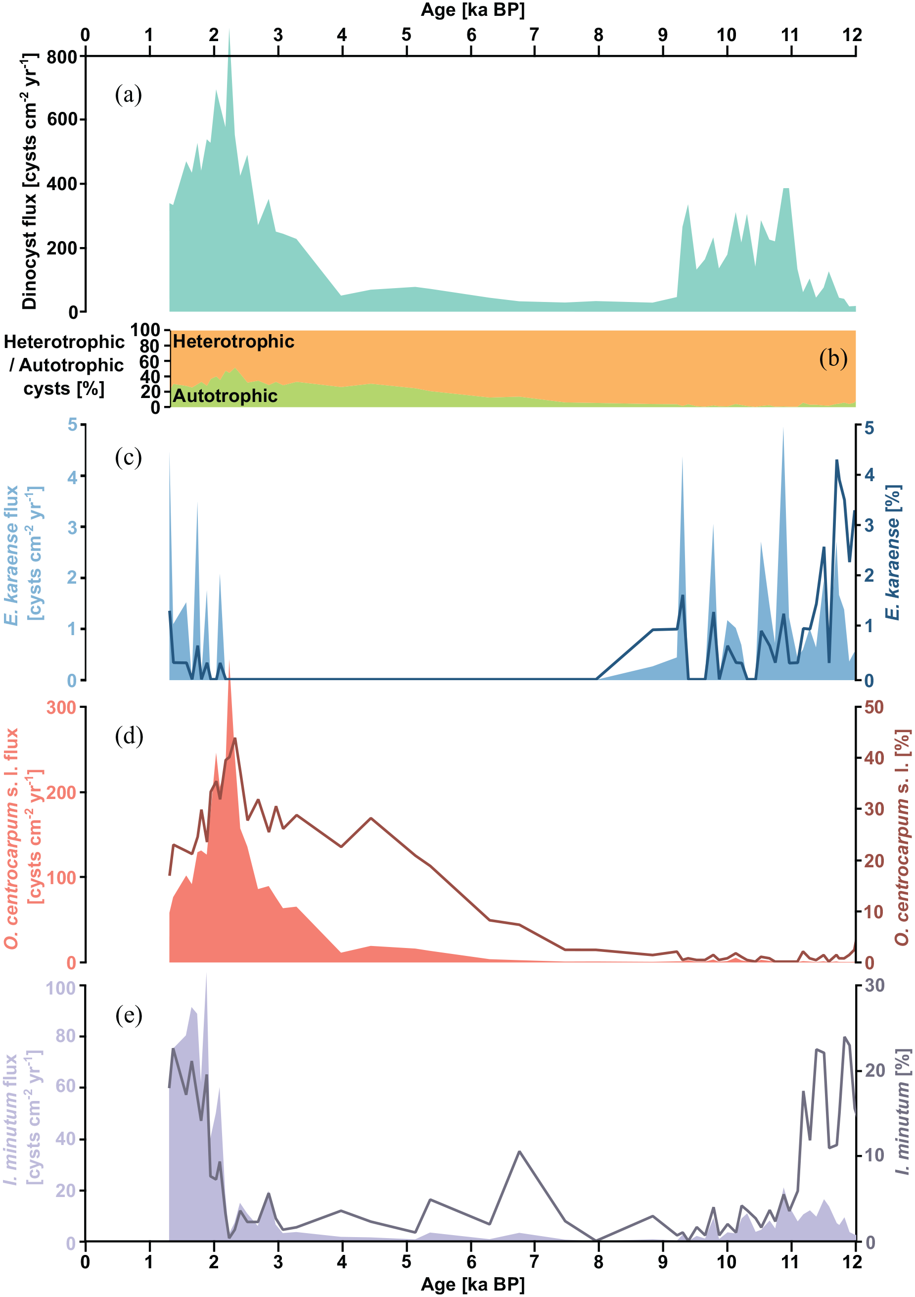
Dinocyst record of core JM09-020. (a) Dinocyst flux [cysts cm⁻² yr⁻¹]. (b) Relative abundance of autotrophic versus heterotrophic species. (c) Flux [cysts cm⁻² yr⁻¹] and relative abundance [%] of Echinidinium karaense. (d) Flux [cysts cm⁻² yr⁻¹] and relative abundance [%] of Operculoidinium centrocarpum s.l. (e) Flux [cysts cm⁻² yr⁻¹] and relative abundance [%] of Islandinium minutum.

Discussion

The dinocyst species Echnidinium karaense, together with cysts of Polarella glacialis, has recently been identified as a winter drift ice indicator in waters around Svalbard (Telesiński et al., 2023). As the latter species is virtually absent in core JM09-020 (Supplemental Material), Echinidinium karaense remains the only available dinocyst sea-ice indicator. It was present in the western Barents Sea over the Early Holocene but it disappeared around 8 ka BP (Figure 2c), indicating ice-free conditions. Its reappearance at around 2.1 ka BP, after almost 6 thousand years of absence, clearly indicates a return of sea-ice conditions comparable to those in the Early Holocene. This is further supported by other dinocyst data from the same core. The peak in autotrophic dinocyst abundance at 2.3 ka BP (Figure 2b), followed by a peak in total dinocyst flux (Figure 2a) shortly thereafter, indicates increased primary productivity, which might suggest that the core site was reached by the MIZ (e.g. Barber et al., 2015; Ramseier et al., 1999; Sakshaug, 2004). After ~2 ka BP the total and autotrophic dinocyst abundance decreased, suggesting deteriorating surface water conditions, possibly due to the thickening of the sea-ice cover. Similarly, the abundance of Operculoidinium centrocarpum s.l., a cosmopolitan species whose high abundances in high northern latitudes are associated with AW dominance (Grøsfjeld et al., 2009; Rochon et al., 1999; Telesiński et al., 2023) reached a maximum around 2.3 ka BP but decreased sharply shortly thereafter, though remained higher than in the first half of the Holocene (Figure 2d). Furthermore, the relative percentage of O. centrocarpum s.l. versus I. minutum, which was relatively high throughout most of the Late-Holocene (Figure 3c), decreased after 2.1 ka BP. The relative percentage of these two species may be used to indicate whether warm AW flows at the surface or as a subsurface water mass (Grøsfjeld et al., 2009). This suggests that until ~2.1 ka BP, AW remained at the surface in the northwestern Barents Sea, while it subducted below ArW thereafter.

Figure 3.

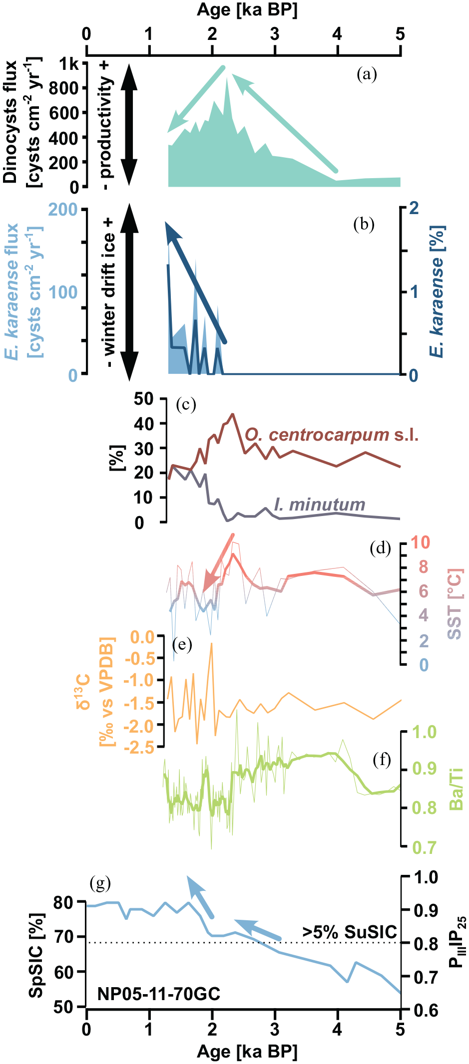
Paleoceanographic proxies of Late-Holocene changes in the northwestern Barents Sea from cores JM09-020 (a–f) and NP05-11-70GC (g). (a) Dinocyst flux [cysts cm⁻² yr⁻¹]. (b) Flux [cysts cm⁻² yr⁻¹] and relative abundance [%] of Echinidinium karaense. (c) Relative [%] abundance of Operculoidinium centrocarpum s.l. and Islandinium minutum. (d) Alkenone-based sea-surface temperature reconstruction (Łącka et al., 2019). Thin line – raw data, thick line – 3 pt moving average. e) Stable carbon isotope ratios [‰ vs VPDB] of benthic foraminifera Elphidium clavatum (Łącka et al., 2015). (f) Ba/Ti elemental ratios obtained from XRF core scanning (Łącka et al., 2015). Thin line – raw data, thick line – 5 pt moving average. (g) P_IIIIP₂₅ index and spring sea-ice concentration (SpSIC) [%] calculated from it (Berben et al., 2017). The horizontal dashed line marks the 0.8 P_IIIIP₂₅ threshold, indicating >5% summer sea-ice concentration.

Additional evidence from core JM09-020 corroborates the dinocyst data. An SST reconstruction based on alkenones (Łącka et al., 2019) shows a clear cooling trend between 2.3 and 2 ka BP (Figure 3d), which could be attributed to the expansion of sea ice. Similarly, the stable carbon isotope values of benthic foraminifera (Łącka et al., 2015) indicate increased variability in environmental conditions after 2 ka BP on the sea bottom (Figure 3e), which could be linked to enhanced sea-ice cover, variable productivity at the sea surface, and the amount of organic matter reaching the sea floor. Further details are provided by XRF data (Łącka et al., 2015). The Ba/Ti ratio exhibits a stepwise decrease around 2.3 ka BP (Figure 3f). Since the Ba/Ti ratio is believed to be broadly proportional to the organic carbon content in sediment (Thomson et al., 2006), such a decrease could indicate declining productivity (Croudace et al., 2006).

Based on the available data, it is evident that the northwestern Barents Sea witnessed a period of maximum productivity around 2.3 ka BP. This was mainly due to the inflow of warm surface AW from the west and the migration of the MIZ from the east. However, after 2.3–2.1 ka BP, the study site was covered with sea ice, and the AW submerged below surface ArW, which resulted in a decrease in SST and productivity.

Our results are further confirmed by data from core NP05-11-70GC from the Olga Basin, east of Svalbard (Berben et al., 2017). The P_IIIIP₂₅ index combines concentrations of tri-unsaturated highly branched isoprenoid (HBI) lipid (HBI III), a phytoplankton-derived biomarker, with IP₂₅, a sea-ice proxy, to investigate past sea-ice conditions more quantitatively (Belt et al., 2007; Berben et al., 2017; Müller et al., 2011). The Olga Basin record indicates a constant increase in sea-ice concentration over the Holocene (Berben et al., 2017). Around 2.8 ka BP, the P_IIIIP₂₅ index crossed the 0.8 threshold (Figure 3g), indicating >5% summer sea-ice concentration (Smik et al., 2016). Around 2.5 ka BP, spring sea-ice concentration in the Olga Basin, derived from the P_IIIIP₂₅ index (Berben et al., 2017), reached 70%. Finally, around 1.9 ka BP, another stepwise increase of the P_IIIIP₂₅ index (approximately equal to eight of the total Holocene increase) occurred. The data from the Olga Basin confirm that a strong environmental gradient characterized the Barents Sea also in the past. While in the northern part of the basin, a dense spring sea-ice concentration was reached already around 2.5 ka BP, in the western part winter drift ice only appeared around 2.1 ka BP (Figure 3b and g). Nevertheless, data from both records confirm that the sea-ice cover reacted slowly to the Neoglacial cooling. Similarly, oxygen isotope data from core NP05-71GC from south of Kvitøya (Klitgaard-Kristensen et al., 2013) suggest that only after c. 2.5 ka BP the northwestern Barents Sea experienced cooling and/or increased brine formation, most probably related to the sea-ice expansion.

All the presented data suggest that the sea-ice expansion in the north-western Barents Sea occurred around 2.5–2.1 ka BP. Such a late response of the sea-ice cover to Neoglacial cooling is surprising. Firstly, the Arctic sea-ice production on the Siberian shelves has reached its modern magnitude already around 5 ka BP (Bauch et al., 2001; Werner et al., 2013) causing perennial sea-ice cover in the Arctic Ocean (Cronin et al., 2010). The fact that the sea-ice cover in the Barents Sea did not respond to this increase can be explained by the minor influence of advected (as opposed to locally formed) sea ice on the basin’s ice budget during the Late-Holocene (Loeng, 1991). On the other hand, terrestrial data indicate that the glacier re-advance in Svalbard began as early as ~4 ka BP (Farnsworth et al., 2020; Jang et al., 2023; Svendsen and Mangerud, 1997), suggesting that the atmospheric cooling in the north-western Barents Sea region required for the glacier growth was already achieved at the beginning of the Late-Holocene.

The approximately 2 kyr delay of the sea-ice expansion relative to the onset of atmospheric cooling and glacier advance in the region indicates that sea-ice cover in the Barents Sea needed significant time to recover, even in favorable climatic conditions. This was probably caused by the strong influence of AW, whose intrusions into the Barents Sea were frequent during the Middle and Late-Holocene (e.g. Pawłowska et al., 2020; Risebrobakken et al., 2010). It is worth noting that in core JM09-020, the abundance of the AW-indicating species Operculoidinium centrocarpum s.l. reached its maximum only ~2.3 ka BP (Figure 3c) and SST as well as productivity remained high until that time (Figure 3d and f), suggesting that in the western Barents Sea, the influence of AW was still increasing well into the Late-Holocene, despite the ongoing expansion of the sea-ice cover in the northern and eastern parts of the basin (Berben et al., 2017).

In the western Barents Sea, the PF is currently mainly topographically controlled (Lien et al., 2017). However, during the warm middle Holocene, the PF most probably decoupled from the bottom topography, allowing AW to reach much farther to the northeast (e.g. Berben et al., 2017). As a result, when orbitally forced Neoglacial cooling began, time was needed to push surface AW out of the central part of the Barents Sea, whereas in the west AW could have even increased its inflow on the surface. Even when atmospheric cooling in the region was advanced enough ~4 ka BP to allow the advance of Svalbard glaciers, another ~2 kyr was needed for the sea surface to cool enough to allow the sea ice to expand into the western Barents Sea. On the other hand, open water in the vicinity of Svalbard must have been an important source of moisture that allowed the growth of the glaciers (e.g. Hebbeln et al., 1994).

Over the last decades, AW intrusions on the Barents Sea shelf have become increasingly common (Kujawa et al., 2021; Telesiński et al., 2023; Walczowski and Piechura, 2011) as a result of enhanced northward heat transfer by the North Atlantic Drift (e.g. Spielhagen et al., 2011; Walczowski and Piechura, 2007), a phenomenon referred to as “Atlantification” of the Barents Sea (e.g. Årthun et al., 2012; Tesi et al., 2021). The delayed response of the sea-ice cover in the Barents Sea to Late-Holocene cooling demonstrated in this study suggests that even if the ongoing global warming is reversed in the future, which in itself is a highly challenging task, many centuries might be required for the sea ice to recover to its preindustrial extent. Taking into account that shrinking sea ice is one of the main drivers of the Arctic amplification (Serreze and Francis, 2006) as it reduces surface albedo, leading to greater surface solar absorption, amplifying warming, and further melt (e.g. Curry et al., 1995; Thackeray and Hall, 2019), the currently observed rapid sea-ice loss (e.g. Overland and Wang, 2013) might be an incredibly slow and long process to reverse.

Summary and conclusions

Reconstructing the paleoceanographic evolution of the northwestern Barents Sea during the Late-Holocene has been made possible by analyzing dinocyst assemblage data from sediment core JM09-020 from Storfjordrenna, south of Svalbard. The dinocyst data has been supplemented by stable carbon isotope, alkenone-based SST, and XRF data that have been previously published (Łącka et al., 2015, 2019). Furthermore, the dinocyst data has been compared with biomarker-based data from core NP05-11-70GC from the Olga Basin, east of Svalbard (Berben et al., 2017).

Based on the data, it appears that despite the ongoing Neoglacial cooling that began around 5 ka BP in high northern latitudes, the northeastern Barents Sea experienced a period of maximum productivity around 2.3 ka BP. This was due to two factors: the dominance of warm AW on the surface, and the proximity of the MIZ. Only after 2.3–2.1 ka BP did winter drift ice begin to cover the northwestern Barents Sea, resulting in a decrease in SST and productivity due to the subduction of AW below ArW.

Our findings have important implications for the current and future environmental changes. The presented data show that the recovery of the sea ice in the Barents Sea is a slow process. Even if the ongoing global warming can be halted or even revoked in the future, the reversing of the present sea-ice loss in the Barents Sea may be an incredibly long process.

Footnotes

Acknowledgements

We would like to express our gratitude to an anonymous reviewer for their helpful feedback and valuable suggestions, which greatly improved the quality of the manuscript.

Funding

The author(s) disclosed receipt of the following financial support for the research, authorship, and/or publication of this article: This study was supported by grant no. 2020/39/B/ST10/01698 funded by the National Science Centre, Poland.

ORCID iD

Maciej M. Telesiński

Supplemental Material

Supplementary Material, containing all the dinocyst data from core JM09-020, is available on Zenodo (https://doi.org/10.5281/zenodo.8322505, Telesiński et al., 2023).

References

Abrahamsen

Østerhus

Gammelsrød

(2006) Ice draft and current measurements from the north-western Barents Sea, 1993–96. Polar Research 25(1): 25–37.

Andersen

Koç

Jennings

, et al. (2004) Nonuniform response of the major surface currents in the Nordic Seas to insolation forcing: Implications for the Holocene climate variability. Paleoceanography 19: A2003.

Andersen

Koç

Moros

(2004) A highly unstable Holocene climate in the subpolar North Atlantic: Evidence from diatoms. Quaternary Science Reviews 23: 2155–2166.

Årthun

Eldevik

Smedsrud

, et al. (2012) Quantifying the influence of Atlantic Heat on Barents Sea ice variability and retreat. Journal of Climate 25(13): 4736–4743.

Bakke

Dahl

Paasche , et al. (2005) Glacier fluctuations, equilibrium-line altitudes and palaeoclimate in Lyngen, northern Norway, during the Lateglacial and Holocene. Holocene 15(4): 518–540.

Barber

Hop

Mundy

, et al. (2015) Selected physical, biological and biogeochemical implications of a rapidly changing Arctic Marginal Ice Zone. Progress in Oceanography 139: 122–150.

Bauch

Mueller-Lupp

Taldenkova

, et al. (2001) Chronology of the Holocene transgression at the North Siberian margin. Global and Planetary Change 31: 125–139.

Belt

Massé

Rowland

, et al. (2007) A novel chemical fossil of palaeo sea ice: IP25. Organic Geochemistry 38: 16–27.

Berben

SMP

Husum

Navarro-Rodriguez

, et al. (2017) Semi-quantitative reconstruction of early to late Holocene spring and summer sea ice conditions in the northern Barents Sea. Journal of Quaternary Science 32(5): 587–603.

10.

Bianchi

McCave

(1999) Holocene periodicity in North Atlantic climate and deep-ocean flow south of Iceland. Nature 397: 515–517.

11.

Bradley

Bakke

(2019) Is there evidence for a 4.2 ka BP event in the northern North Atlantic region? Climate of the Past 15: 1665–1676.

12.

Cronin

Gemery

Briggs

, et al. (2010) Quaternary sea-ice history in the Arctic Ocean based on a new ostracode sea-ice proxy. Quaternary Science Reviews 29(25-26): 3415–3429.

13.

Croudace

Rindby

Rothwell

(2006) ITRAX: Description and evaluation of a new multi-function X-ray core scanner. Geological Society Special Publication 267: 51–63.

14.

Curry

Schramm

Ebert

(1995) Sea Ice-Albedo climate feedback mechanism. Journal of Climate 8(2): 240–247.

15.

Dahl-Jensen

Mosegaard

Gundestrup

, et al. (1998) Past temperatures directly from the Greenland Ice Sheet. Science 282(5387): 268–271.

16.

Divine

Dick

(2006) Historical variability of sea ice edge position in the Nordic Seas. Journal of Geophysical Research Oceans 111(C1): 1–14.

17.

Dyke

England

Reimnitz

, et al. (1997) Changes in driftwood delivery to the Canadian Arctic Archipelago: The hypothesis of postglacial oscillations of the transpolar drift. Arctic 50(1): 1–16.

18.

Farnsworth

Allaart

Ingólfsson , et al. (2020) Holocene glacial history of Svalbard: Status, perspectives and challenges. Earth-Science Reviews 208: 103249.

19.

Giraudeau

Grelaud

Solignac

, et al. (2010) Millennial-scale variability in Atlantic water advection to the Nordic seas derived from Holocene coccolith concentration records. Quaternary Science Reviews 29(9-10): 1276–1287.

20.

Grøsfjeld

Harland

Howe

(2009) Dinoflagellate cyst assemblages inshore and offshore Svalbard reflecting their modern hydrography and climate. Norwegian Journal of Geology 89(1–2): 121–134.

21.

Head

Harland

Matthiessen

(2001) Cold marine indicators of the late Quaternary: The new dinoflagellate cyst genus Islandinium and related morphotypes. Journal of Quaternary Science 16(7): 621–636.

22.

Heaton

Bard

Bronk Ramsey

, et al. (2022) A response to community questions on the marine20 radiocarbon age calibration curve: Marine reservoir ages and the calibration of 14 C samples from the oceans. Radiocarbon 00(1): 00–27.

23.

Heaton

Köhler

Butzin

, et al. (2020) Marine20 — the Marine Radiocarbon Age Calibration Curve (0 – 55,000 Cal Bp). Radiocarbon 62(4): 779–820.

24.

Hebbeln

Dokken

Andersen

, et al. (1994) Moisture supply for northern ice-sheet growth during the Last Glacial Maximum. Nature 370: 357–360.

25.

Hebbeln

Wefer

(1991) Effects of ice coverage and ice-rafted material on sedimentation in the Fram Strait. Nature 350: 409–411.

26.

Hopkins

(1991) The GIN Sea—A synthesis of its physical oceanography and literature review 1972–1985. Earth-Science Reviews 30(3-4): 175–318.

27.

Jang

Bayon

Vogt

, et al. (2023) Non-linear response of glacier melting to Holocene warming in Svalbard recorded by sedimentary iron (oxyhydr)oxides. Earth and Planetary Science Letters 607: 118054.

28.

Johnsen

Dahl-Jensen

Gundestrup

, et al. (2001) Oxygen isotope and palaeotemperature records from six Greenland ice-core stations: camp Century, dye-3, GRIP, GISP2, Renland and NorthGRIP. Journal of Quaternary Science 16(4): 299–307.

29.

Klitgaard-Kristensen

Rasmussen

Koç

(2013) Palaeoceanographic changes in the northern Barents Sea during the last 16 000 years – New constraints on the last deglaciation of the Svalbard–Barents Sea Ice Sheet. Boreas 42(3): 798–813.

30.

Knies

Pathirana

Cabedo-Sanz

, et al. (2017) Sea-ice dynamics in an Arctic coastal polynya during the past 6500 years. Arktos 3(1): 1.

31.

Kujawa

Łącka

Szymańska

, et al. (2021) Could Norwegian fjords serve as an analogue for the future of the Svalbard fjords? State and fate of high latitude fjords in the face of progressive “atlantification.” Polar Biology 44(12): 2217–2233.

32.

Kunz-Pirrung

(1998) Rekonstruktion der Oberflächenwassermassen der östlichen Laptevsee im Holozän anhand von aquatischen Palynomorphen. Berichte zur Polarforschung 281: 1–117.

33.

Łącka

Cao

Rosell-Melé

, et al. (2019) Postglacial paleoceanography of the western Barents Sea: Implications for alkenone-based sea surface temperatures and primary productivity. Quaternary Science Reviews 224: 105973. DOI: 10.1016/j.quascirev.2019.105973

34.

Łącka

Michalska

Pawłowska

, et al. (2020) Multiproxy paleoceanographic study from the western Barents Sea reveals dramatic Younger Dryas onset followed by oscillatory warming trend. Scientific Reports 10(1): 15667.

35.

Łącka

Zajączkowski

Forwick

, et al. (2015) Late Weichselian and Holocene palaeoceanography of Storfjordrenna, southern Svalbard. Climate of the Past 11: 587–603.

36.

Laskar

Robutel

Joutel

, et al. (2004) A long-term numerical solution for the insolation quantities of the Earth. Astronomy and Astrophysics 428(1): 261–285.

37.

Lien

Schlichtholz

Skagseth , et al. (2017) Wind-driven Atlantic water flow as a direct mode for reduced Barents Sea ice cover. Journal of Climate 30(2): 803–812.

38.

Loeng

(1991) Features of the physical oceanographic conditions of the Barents Sea. Polar Research 10(1): 5–18.

39.

Mangerud

Bondevik

Gulliksen

, et al. (2006) Marine 14C reservoir ages for 19th century whales and molluscs from the North Atlantic. Quaternary Science Reviews 25(23-24): 3228–3245.

40.

Manley

(1995) Branching of Atlantic water within the Greenland-Spitsbergen Passage: An estimate of recirculation. Journal of Geophysical Research 100(C10): 20,627–20,634.

41.

Matul

Spielhagen

Kazarina

, et al. (2018) Warm-water events in the eastern Fram Strait during the last 2000 years as revealed by different microfossil groups. Polar Research 37(1): 1540243. DOI: 10.1080/17518369.2018.1540243

42.

McDermott

Mattey

Hawkesworth

(2001) Centennial-scale Holocene climate variability revealed by a high-resolution speleothem delta 18O record from SW Ireland. Science 294: 1328–1331.

43.

McKay

Kaufman

Routson

, et al. (2018) The onset and rate of Holocene neoglacial cooling in the Arctic. Geophysical Research Letters 45(22): 12,487–12,496.

44.

Mertens

Price

Pospelova

(2012b) Determining the absolute abundance of dinoflagellate cysts in recent marine sediments II: Further tests of the Lycopodium marker-grain method. Review of Palaeobotany and Palynology 184: 74–81.

45.

Mertens

Rengefors

Moestrup

, et al. (2012a) A review of recent freshwater dinoflagellate cysts: Taxonomy, phylogeny, ecology and palaeocology. Phycologia 51(6): 612–619.

46.

Mertens

Takano

, et al. (2015) Cyst-theca relationship of a new dinoflagellate with a spiny round brown cyst, Protoperidinium lewisiae sp. Nov., and its comparison to the cyst of Oblea acanthocysta. Phycological Research 63(2): 110–124.

47.

Mertens

Verhoeven

Verleye

, et al. (2009) Determining the absolute abundance of dinoflagellate cysts in recent marine sediments: The Lycopodium marker-grain method put to the test. Review of Palaeobotany and Palynology 157(3-4): 238–252.

48.

Mertens

Yamaguchi

Takano

, et al. (2013) A new heterotrophic dinoflagellate from the north-eastern Pacific, Protoperidinium fukuyoi: Cyst-theca relationship, phylogeny, distribution and ecology. Journal of Eukaryotic Microbiology 60(6): 545–563.

49.

Moestrup Lindberg

Daugbjerg

(2009) Studies on woloszynskioid dinoflagellates IV: The genus Biecheleria gen. nov. Phycological Research 57(3): 203–220.

50.

Montresor

Procaccini

Stoecker

(1999) Polarella glacialis, gen. nov., sp. nov. (Dinophyceae): Suessiaceae are still alive! Journal of Phycology 35: 186–197.

51.

Müller

Wagner

Fahl

, et al. (2011) Towards quantitative sea ice reconstructions in the northern North Atlantic: A combined biomarker and numerical modelling approach. Earth and Planetary Science Letters 306(3-4): 137–148.

52.

Müller

Werner

Stein

, et al. (2012) Holocene cooling culminates in sea ice oscillations in Fram Strait. Quaternary Science Reviews 47: 1–14.

53.

Olsen

Anderson

Knudsen

(2012) Variability of the North Atlantic oscillation over the past 5,200 years. Nature Geoscience 5(11): 808–812.

54.

Orme

Miettinen

Divine

, et al. (2018) Subpolar North Atlantic sea surface temperature since 6 ka BP: Indications of anomalous ocean-atmosphere interactions at 4-2 ka BP. Quaternary Science Reviews 194: 128–142.

55.

Overland

Wang

(2013) When will the summer Arctic be nearly sea ice free? Geophysical Research Letters 40(10): 2097–2101.

56.

Paasche Bakke

(2009) The Holocene turnover - A global climatic shift at ~4 Ka. Geophysical Research Abstracts 11: EGU2009-14017. Available at: https://meetings.copernicus.org/egu2009/

57.

Paasche Løvlie

Dahl

, et al. (2004) Bacterial magnetite in lake sediments: Late glacial to Holocene climate and sedimentary changes in northern Norway. Earth and Planetary Science Letters 223(3-4): 319–333.

58.

Pawłowska

Łącka

Kucharska

, et al. (2020) Multiproxy evidence of the neoglacial expansion of Atlantic Water to eastern Svalbard. Climate of the Past 16(2): 487–501.

59.

Pfirman

Bauch

Gammelsrød

(1994) The Northern Barents Sea: Water mass distribution and modification. In: Johannessen

Muench

Overland

(eds) The Polar Oceans and Their Role in Shaping the Global Environment, vol. 85. Geophysica: American Geophysical Union, pp.77–94.

60.

Pospelova

Chmura

Boothman

, et al. (2005) Spatial distribution of modern dinoflagellate cysts in polluted estuarine sediments from Buzzards Bay (Massachusetts, USA) embayments. Marine Ecology Progress Series 292(Taylor 1987): 23–40.

61.

Pospelova

Esenkulova

Johannessen

, et al. (2010) Organic-walled dinoflagellate cyst production, composition and flux from 1996 to 1998 in the central Strait of Georgia (BC, Canada): A sediment trap study. Marine Micropaleontology 75(1-4): 17–37.

62.

Pospelova

Head

(2002) Islandinium brevispinosum sp. nov. (Dinoflagellata), a new organic-walled dinoflagellate cyst from modern estuarine sediments of new England (USA). Journal of Phycology 38(3): 593–601.

63.

Prange

Lohmann

(2003) Effects of Mid-Holocene river runoff on the Arctic ocean/sea-ice system: A numerical model study. Holocene 13(3): 335–342.

64.

Ramseier

Garrity

Bauerfeind

, et al. (1999) Sea-ice impact on long-term particle flux in the Greenland Sea’s is Odden-Nordbukta region, 1985–1996. Journal of Geophysical Research 104(C3): 5329–5343.

65.

Reimer

(2001) A marine reservoir correction database and on-line interface. Radiocarbon 43(2A): 461–463.

66.

Renssen

(2022) Climate model experiments on the 4.2 ka event: The impact of tropical sea-surface temperature anomalies and desertification. Holocene 32(5): 378–389.

67.

Rigual-Hernández

Colmenero-Hidalgo

Martrat

, et al. (2017) Svalbard ice-sheet decay after the Last Glacial Maximum: New insights from micropalaeontological and organic biomarker paleoceanographical reconstructions. Palaeogeography Palaeoclimatology Palaeoecology 465: 225–236.

68.

Risebrobakken

Moros

Ivanova

, et al. (2010) Climate and oceanographic variability in the SW Barents Sea during the Holocene. Holocene 20(4): 609–621.

69.

Rochon

de Vernal

Turon

, et al. (1999) Distribution of recent dinoflagellate cysts in surface sediments from the North Atlantic Ocean and adjacent seas in relation to sea-surface parameters. American Association of Stratigraphic Palynologists Contribution Series 35: 1–146.

70.

Rudels

Korhonen

Schauer

, et al. (2015) Circulation and transformation of Atlantic water in the Eurasian Basin and the contribution of the Fram Strait inflow branch to the Arctic Ocean heat budget. Progress in Oceanography 132: 128–152.

71.

Sakshaug

(2004) Primary and secondary production in the Arctic Seas. In: Stein

Macdonald

(eds) The Organic Carbon Cycle in the Arctic Ocean. Berlin, Heidelberg: Springer, pp.57–81.

72.

Sarnthein

van Kreveld

Erlenkeuser

(2003) Centennial-to-millennial-scale periodicities of Holocene climate and sediment injections off the western Barents shelf, 75°N. Boreas 32: 447–461.

73.

Schauer

Loeng

Rudels

, et al. (2002) Atlantic water flow through the Barents and Kara Seas. Deep-Sea Research Part I: Oceanographic Research Papers 49(12): 2281–2298.

74.

Serreze

Francis

(2006) The Arctic amplification debate. Climatic Change 76(3-4): 241–264.

75.

Smik

Cabedo-Sanz

Belt

(2016) Semi-quantitative estimates of paleo Arctic sea ice concentration based on source-specific highly branched isoprenoid alkenes: A further development of the PIP25 index. Organic Geochemistry 92: 63–69.

76.

Smith

Jr Sakshaug

(1990) Polar phytoplankton. In: Smith

Jr (ed.) Polar Oceanography. New York: Academic Press, pp.477–525.

77.

Sorteberg

Kvingedal

(2006) Atmospheric forcing on the Barents Sea winter ice extent. Journal of Climate 19(19): 4772–4784.

78.

Spielhagen

Werner

Sørensen

, et al. (2011) Enhanced modern heat transfer to the Arctic by warm Atlantic Water. Science 331: 450–453.

79.

Stuiver

Reimer

(1993) Radiocarbon calibration program. Radiocarbon 35: 215–230.

80.

Svendsen

Mangerud

(1997) Holocene glacial and climatic variations on Spitsbergen, Svalbard. Holocene 7(1): 45–57.

81.

Telesiński

Bauch

Spielhagen

, et al. (2015) Evolution of the central Nordic Seas over the last 20 thousand years. Quaternary Science Reviews 121: 98–109.

82.

Telesiński

Pospelova

Mertens

, et al. (2023) Dinoflagellate cysts and benthic foraminifera from surface sediments of Svalbard fjords and shelves as paleoenvironmental indicators. Oceanologia 65(4): 571–594.

83.

Telesiński

Spielhagen

Bauch

(2014) Water mass evolution of the Greenland Sea since late glacial times. Climate of the Past 10: 123–136.

84.

Tesi

Muschitiello

Mollenhauer

, et al. (2021) Rapid Atlantification along the Fram Strait at the beginning of the 20th century. Science Advances 7(48): eabj2946.

85.

Thackeray

Hall

(2019) An emergent constraint on future Arctic sea-ice albedo feedback. Nature Climate Change 9(12): 972–978.

86.

Thomson

Croudace

Rothwell

(2006) A geochemical application of the ITRAX scanner to a sediment core containing eastern Mediterranean sapropel units. Geological Society Special Publication 267: 65–77.

87.

Vinje

(1977) Sea ice conditions in the European sector of the marginal seas of the Arctic, 1966-1975. Norsk Polarinstitut Årbok 1975: 163–174.

88.

Vinje

(2001) Anomalies and trends of sea-ice extent and atmospheric circulation in the Nordic Seas during the period 1864–1998. Journal of Climate 14(3): 255–267.

89.

Walczowski

Piechura

(2007) Pathways of the Greenland Sea warming. Geophysical Research Letters 34(10): 5.

90.

Walczowski

Piechura

(2011) Influence of the West Spitsbergen current on the local climate. International Journal of Climatology 31(7): 1088–1093.

91.

Walker

Head

Lowe

, et al. (2019) Subdividing the Holocene Series/Epoch: Formalization of stages/ages and subseries/subepochs, and designation of GSSPs and auxiliary stratotypes. Journal of Quaternary Science 34(3): 173–186.

92.

Wang

Surge

Mithen

(2012) Seasonal temperature variability of the neoglacial (3300–2500BP) and Roman warm period (2500–1600BP) reconstructed from oxygen isotope ratios of limpet shells (Patella vulgata), Northwest Scotland. Palaeogeography Palaeoclimatology Palaeoecology 317-318: 104–113.

93.

Wanner

(2021) Late-Holocene: Cooler or warmer? Holocene 31(9): 1501–1506.

94.

Wassmann

(2011) Arctic marine ecosystems in an era of rapid climate change. Progress in Oceanography 90(1-4): 1–17.

95.

Wassmann

Reigstad

Haug

, et al. (2006) Food webs and carbon flux in the Barents Sea. Progress in Oceanography 71(2-4): 232–287.

96.

Werner

Spielhagen

Bauch

, et al. (2013) Atlantic water advection versus sea-ice advances in the eastern Fram Strait during the last 9 ka: Multiproxy evidence for a two-phase Holocene. Paleoceanography 28: 283–295.

97.

Zonneveld

KAF

(1997) New species of organic walled dinoflagellate cysts from modern sediments of the Arabian Sea (Indian Ocean). Review of Palaeobotany and Palynology 97(3-4): 319–337.

98.

Zonneveld

KAF

Pospelova

(2015) A determination key for modern dinoflagellate cysts. Palynology 39(3): 387–409.

A late response of the sea-ice cover to Neoglacial cooling in the western Barents Sea

Abstract

Keywords

Introduction

Oceanographic setting

Material and methods

Results

Discussion

Summary and conclusions

Footnotes

Acknowledgements

Funding

ORCID iD

Supplemental Material

References