Sage Journals: Discover world-class research

Abstract

The late-Quaternary relative sea-level (RSL) history of Ireland is complex, positioned at the margins of the former British-Irish Ice Sheet, and subject to the influence of ice unloading and forebulge collapse. Geophysical models of post-glacial isostatic adjustment (GIA) provide estimates of the pattern of RSL change since deglaciation which may be tested and validated with empirical data from proxy records. For the region of northwest Ireland, there is a paucity of high-quality RSL data and, therefore, equivocal evidence to support the GIA models that predict a mid to Late-Holocene RSL highstand of between +0.5 and +2 m above present. This study aims to investigate this model-data discrepancy by reconstructing RSL change from a near continuous salt-marsh sequence at Bracky Bridge, Donegal, spanning the last ca. 2500 years. We develop a transfer function model to reconstruct the vertical position of sea level using a regional diatom training set to quantify the indicative meaning and predict the palaeomarsh elevation of the core samples. A chronology is provided by a combination of ¹⁴C and ²¹⁰Pb data, with sample specific ages derived from an age-depth model using a Bayesian framework. Our reconstruction shows ca. 2 m of relative sea-level rise in the past 2500 years. This is not compatible with some previously published sea-level index points from the region, which we re-interpret as freshwater/terrestrial limiting data. These results do not provide any evidence to support a Mid-Holocene RSL highstand above present sea level. Whilst none of the available GIA models replicate the timing and magnitude of the Late-Holocene RSL rise in our reconstruction, those which incorporate a thick and extensive British-Irish Sea Ice Sheet provide the best fit.

Keywords

diatom foraminifera microfossil relative sea level transfer function

Introduction

Regional patterns of Holocene relative sea-level (RSL) change around the British Isles are strongly controlled by glacial isostatic adjustment (GIA). The magnitude of the GIA signal is related to the growth and retreat of former ice sheets and, as such, is spatially and temporally variable. Lying at the periphery of two former ice sheets (i.e. the British-Irish and the larger Fennoscandian ice sheets) and subject to the influence of proglacial forebulge collapse, the British Isles occupies a complex and isostatically transitional area between uplift and subsidence, providing a key testing ground for GIA models. Holocene relative sea-level data from geological archives in regions which straddle the boundaries between uplift and subsidence arguably provide the most sensitive tests for these models (Rushby et al., 2019).

In contrast to Britain, where a high-quality and widely distributed database of Holocene RSL observations has been compiled (Shennan et al., 2018), there remains a paucity of RSL data for Ireland, with the available record fragmentary, both in terms of geographical spread and temporal range. In particular, sites in western Ireland are rare and most constraints on sea level are currently of low resolution, with large uncertainties or limited quantification of the relationship between the sea-level indicator and contemporaneous tidal levels (i.e. the indicative meaning) (Brooks et al., 2008). Studies by Shaw and Carter (1994) and Carter et al. (1989) allow broad patterns of Holocene RSL and coastal evolution to be constrained, and have more recently been supplemented by further RSL data (Edwards et al., 2017). Nevertheless, significant gaps between the field data and GIA modelling persist.

To address the scarcity and poor resolution of existing RSL data from northwest Ireland, in this paper we seek to derive a new high-resolution proxy-based RSL reconstruction from a salt marsh in western Donegal. For the first time at any site in Ireland, we reconstruct sea-level changes from a continuous salt-marsh sequence dating back 2500 years using a quantitative transfer function approach. This contrasts with previous studies that have, to date, only provided discrete estimates of the position of relative sea levels at particular points in time, rather than a near-continuous reconstruction from which both the patterns and rates of RSL changes may be discerned. Our reconstruction and an updated interpretation of existing sea-level data from the region together provide a robust dataset against which GIA models can be tested and validated. We undertake an initial assessment of the performance of several published GIA models and highlight the implications for understanding the extent and thickness of the last British-Irish Ice Sheet.

Study area

Sedimentary environments along the west coast of Ireland are typically sandy, dynamic and storm dominated due to their exposed aspect (Delaney and Devoy, 1995; Duffy and Devoy, 1998). Nevertheless, low energy embayments are present in sheltered locations, providing suitable conditions for the formation of salt marshes and the accumulation of fine-grained and organic sediments (Curtis and Skeffington, 1998). Based on previous studies (Gallagher et al., 1996; Wheeler et al., 1999), we identified the tidal marsh at Bracky Bridge (54.756°–8.433°, Figure 1) as having a suitable sedimentary record for developing relative sea-level reconstructions using a quantitative biostratigraphic approach. Bracky Bridge is located near to the village of Ardara in County Donegal, around 50 km north of Donegal town. The site is situated at the head of Loughros Beg estuary, within the Slieve Tooey/Tomore Island/Loughros Beg Bay special area of conservation.

Figure 1.

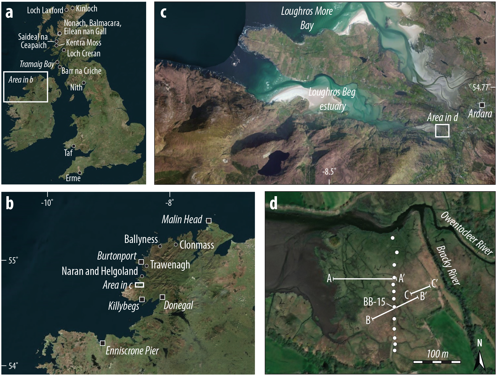
Location of Bracky Bridge, County Donegal, northwest Ireland. (a) Locations of published modern diatom samples used to develop a regional training set; (b) Location of Donegal town, tide gauges (squares, italics), and sites with published sea-level data (dots); (c) Loughros Beg estuary; (d) the salt marsh at Bracky Bridge with surface sample transects A-A’, B-B’ and C-C’ and the coring transect (white dots) marked.

The head of Loughros Beg estuary is framed by quartzite, schist and diamictite of the Loughros and Port Askaig formations, with till mantling the bedrock to the north and south of the Bracky Bridge marsh (Geological Survey of Ireland, 2022). The estuary is sand-filled and characterised by extensive intertidal flats with low-tide ebb channels (Burningham and Cooper, 2004). These channels are dynamic in their behaviour in the lower estuary, but stable in the upper reaches over centennial timescales (Burningham, 2008). A small area of salt marsh, covering approximately 0.1 km² (Figure 1d), occupies the head of the estuary. The Bracky River borders the marsh on its eastern side, before merging with the Owentocleer River and flowing across the northern margin of the site. Grazed fields occupy elevations above the reach of tides to the south of the marsh.

The mean annual rainfall in the catchment is approximately 1600 mm yr⁻¹ (Met Éireann, 2022) and the catchment is approximately 48 km² in area (Burningham and Cooper, 2004). The wet climate is reflected in the salt-marsh vegetation, which does not display particularly distinct halophytic zonation and is dominated by Juncus maritimus (Sheehy Skeffington and Wymer, 1991; Wheeler et al., 1999). Grasses, including Puccinellia maritima, are encountered at lower elevations of the marsh, while the transition to the freshwater zone is marked by the dominance of bryophytes. Human impacts are limited at present, although cows infrequently graze the marsh (Wheeler et al., 1999).

The Donegal coast is mesotidal. While the closest permanent tide gauges to Bracky Bridge are located 100 km to the northeast (Malin Head) and 75 km to the southwest (Enniscrone Pier), the UK Admiralty provides predictions for Loughros More Bay, less than 10 km to the northwest of Bracky Bridge (United Kingdom Hydrographic Office, 2016). Mean high water of spring tides (MHWST), a key datum for comparison of modern microfossil assemblages between sites (Barlow et al., 2013; Zong and Horton, 1999), lies 4.0 m above chart datum. While no data are available for the elevation of Mean Tide Level (MTL) with respect to chart datum, interpolation between Admiralty predictions for Burtonport and Killybegs (locations in Figure 1b) indicates MTL is around 2.13 m, giving a MTL to MHWST range of 1.87 m. As MTL is within ±0.03 m of 0 m Ordnance Datum Malin (ODM) at both Burtonport and Killybegs (Neill, 2020), no adjustment is required to convert from ODM to m MTL.

We do not currently have data to establish whether up-estuary tidal amplification or dampening occurs. Such modification to the tidal range in the present day would influence the calculation of standardised elevations during the development of regional transfer functions (see Statistical analysis and transfer function development section), but would not influence rates of reconstructed RSL change. Nevertheless, changes in tidal range over time would introduce additional uncertainties into reconstructions and are evaluated in the discussion section.

Gallagher et al. (1996) and Wheeler et al. (1999) previously investigated the stratigraphic record of the site. While the Bracky River crosses the northern margin of the site at present, these stratigraphic investigations suggest the position of the river channel has changed over time and previously occupied a position at the south of the marsh. While the seaward edge of the tidal marsh is formed by a cliff approximately 0.7 m high, the location of the marsh edge has remained relatively unchanged since at least 1835 CE (Gallagher et al., 1996).

Methods

Modern microfossil distributions

To characterise the distributions of foraminifera and diatoms in the contemporary environment and develop approaches for reconstructing relative sea level from fossil sequences (see Statistical analysis and transfer function development section), we investigate a training set of samples from the modern marsh surface. The 1 cm-thick modern samples were taken from stations arranged along three transects ranging from the lowest vegetated marsh to the freshwater zone above the limit of tides (Figure 1). Levelling to a temporary benchmark, which was later surveyed using a differential Global Positioning System, provided the elevation of each sample. We express all elevations relative to Ordnance Datum Malin (ODM), the mean sea level at Malin Head between 1960 and 1969.

We prepared samples for the identification and quantification of foraminifera following the methods of Scott and Medioli (1980). We added rose Bengal at the time of sampling to differentiate between live and dead foraminifera (Walton, 1955), sieved samples to between 63 and 500 μm, split samples using a wet splitter (Scott and Hermelin, 1993), and picked specimens under water. Species identifications follow Murray (1971, 1979). Where densities were sufficient, we counted a minimum of 200 specimens. Where this total could not be achieved in a single 1/8 split, we counted further splits or the entire sample. Kemp et al. (2020) conclude that transfer function performance stabilises at lower total count sizes; therefore, we focus our presentation of results on samples with dead counts exceeding 30 specimens.

We analysed diatom assemblages following the preparation and analysis methods of Palmer and Abbott (1986) and Battarbee et al. (2001). Species identifications were made with reference to Krammer and Lange-Bertalot (1991, 1997) as a primary source, supplemented by Van der Werff and Huls (1958) and Hartley (1996). Nomenclature conforms with the World Register of Marine Species (WoRMS Editorial Board, 2022). Total counts exceeded 300 for all samples and we include all species’ relative abundances in subsequent statistical analyses, with no transformation. Salinity classifications follow Denys (1991) and Vos and de Wolf (1993).

Stratigraphy and biostratigraphy

Tidal marshes have the potential to preserve long and continuous records of relative sea-level change in their stratigraphy (Barlow et al., 2013; Shennan, 1982). We conducted reconnaissance coring of the Bracky Bridge marsh using a closely spaced transect of hand-driven gouge cores (Figure 1), with sediments logged using the Troels-Smith system of sediment classification (Troels-Smith, 1955). Levelling to the benchmark provided the elevation of the top of each core. We recovered a representative core and selected basal samples for subsequent laboratory analyses using a 5 cm-diameter Russian-type corer. All core sections and basal samples were stored in flexible non-PVC plastic wrap, with rigid plastic tubing to provide protection, and refrigerated in the dark at 4°C before further analyses.

We prepared and analysed core and basal samples for foraminifera and diatoms following the same methods as applied to the modern samples (see Modern microfossil distributions section). Each core subsample was 1 cm thick, with a resolution increasing from one sample every 4 cm at the base of the core to contiguous samples in the uppermost 20 cm.

Statistical analysis and transfer function development

We investigate clustering in the modern microfossil datasets using the Partitioning Around Medoids (PAM) algorithm (Kaufman and Rousseeuw, 1990; Rousseeuw and Kaufman, 1987) in Matlab v.2019b, testing for 2–10 clusters and accepting the optimum number that provides the highest average silhouette width. Detrended Correspondence Analysis (DCA; Hill and Gauch, 1980) provides a complementary approach for visualising clustering; we conduct this in the CANOCO software package v.4.54 (Ter Braak and Smilauer, 2002). Detrended Canonical Correspondence Analysis (DCCA; Ter Braak, 1986) in CANOCO quantifies the variance in the assemblage data explained by elevation and indicates the rate of species turnover along the elevation gradient.

Transfer functions relate the distribution of a selected microfossil group to an explanatory environmental variable, with the subsequent calibration step providing predictions of the environmental variable from fossil assemblage data along with sample-specific uncertainties (Imbrie and Kipp, 1971; Kemp et al., 2015). We relate the distribution of microfossil assemblages to marsh-surface elevation, seeking models that can then predict the elevation at which a fossil assemblage was most likely deposited, known as the palaeomarsh-surface elevation. The length of the first DCCA axis guides the selection of suitable model types for transfer function development, with lengths >2 σ favouring the use of unimodal rather than linear approaches (Birks, 1995).

The appropriate spatial scale of modern training sets has been widely debated (Gehrels et al., 2001; Hocking et al., 2017; Horton and Edwards, 2005; Watcham et al., 2013; Woodroffe and Long, 2010). Local training sets containing a smaller number of samples from a single site typically provide smaller uncertainties, while larger ‘regional’ training sets incorporating samples from multiple sites characterise a broader range of environments and, therefore, potentially provide better analogues for fossil assemblages. We assess whether our local training set provides an appropriate range of analogues for fossil samples by calculating minimum dissimilarity coefficients (MinDC) using the squared chord distance metric (Birks, 1995) in the Rioja R package (Juggins, 2015). The 20th percentile of the minimum dissimilarities between the modern samples provides the boundary between fossil samples classed as having ‘poor’ analogues and those with fair analogues, while the fifth percentile is the boundary between those with ‘fair’ and ‘good’ analogues (Watcham et al., 2013).

To increase the potential availability of good modern analogues for fossil samples, we combine the Bracky Bridge surface samples with published diatom assemblages from sites in western Scotland (Barlow et al., 2013; Shennan et al., 1995; Innes et al., 1996; Zong and Horton, 1999), south Wales (Gehrels et al., 2001) and southwestern England (Gehrels et al., 2001). Together, this regional diatom training set consists of 323 samples from 13 sites (Figure 1) and forms part of a larger UK diatom training set that also includes samples from the east coast of England (Woodroffe et al., submitted). To account for differences in tidal range and, therefore, the vertical distribution of diatom assemblages between sites, we use a standardised water level index (SWLI) as the environmental variable, scaled to the vertical range between mean tide level (MTL) and mean high water of spring tides (MHWST) at each site (Zong and Horton, 1999). Increasing the number and diversity of samples within a training set moves the modern MinDC percentile boundaries, leading to a higher likelihood of finding analogues that would be classed as ‘good’. We therefore also look for an absolute decrease in MinDC values and identify the location of the closest analogues for each fossil sample to ensure that the regional training set does indeed offer an improvement over the local training set.

We develop transfer functions from the Bracky Bridge and Regional training sets using Weighted Averaging (WA; Ter Braak, 1987) and Weighted Averaging Partial Least Squares (WAPLS; Ter Braak and Juggins, 1993) in the Rioja R package. Transfer functions based on regional training sets often provide lower levels of precision (i.e. larger cross-validated errors) due to increased variability in assemblages unrelated to elevation. To address this, we develop locally weighted (LW) transfer functions that dynamically select the most similar modern samples to each fossil sample and generate a series of unique transfer functions using WAPLS (i.e. LW-WAPLS). The modern samples are selected using their minimum dissimilarity coefficients (chord squared distance metric) and we specify that each successive model contains the 50 closest modern samples, following Birks (2012). We develop the locally weighted model using the R code of Rush et al. (2021). For all models, we use a 1000-cycle bootstrapping approach for cross validation.

We select the final transfer function model for calibrating fossil assemblages based on the cross-validated correlation between observed and predicted elevations (r²_boot), the root mean squared error of prediction (RMSEP), and the distribution of residual differences between observed and predicted elevations. We do not remove any samples based on their bootstrapped residuals. For WAPLS models, we accept the minimum adequate model, only considering the addition of a further component when it offers a decrease in RMSEP exceeding 5% (Barlow et al., 2013; Birks et al., 1998).

Bayesian approaches offer an alternative to classical transfer function models, alleviating the need to decide between linear and unimodal representations of species’ distributions (Cahill et al., 2016). While Bayesian models are beginning to be used for proxy-based sea-level reconstruction, all studies to date have focussed on foraminiferal training sets with species’ diversities often two orders of magnitude lower than the diatom dataset presented here. Due to the computational expense associated with such a large dataset, we do not investigate Bayesian approaches.

Chronology

We develop an age-depth model for the Bracky Bridge core by combining accelerator mass spectrometry (AMS) radiocarbon dating and radionuclide analyses. Radiocarbon samples consisted of horizontally bedded detrital terrestrial plant material that were dated at the Aarhus AMS Dating Centre, Aarhus University, Denmark. We report dates as conventional radiocarbon ages (¹⁴C years before present) and calibrate to calendar years using the IntCal20 calibration curve (Reimer et al., 2020). In addition to the radiocarbon dates from the core, we dated three further basal samples, including one bulk sample.

Supplementing the radiocarbon data in the upper part of the core, we use the short-lived radionuclide ²¹⁰Pb to refine the age model. We determined the activities of ²¹⁰Pb and its parent isotope ²²⁶Ra in contiguous 1 cm samples from the uppermost 30 cm. After freeze drying and homogenisation, radio-isotopes were measured by gamma spectroscopy using a Canberra low-energy Germanium detector at the Dunstaffnage Laboratory of the Scottish Marine Association in Oban, UK. We also ascertained activities of ¹³⁷Cs, which can be used as a marker of the early 1950s onset and 1963 CE peak in atmospheric nuclear weapons testing, alongside other fallout peaks including the 1986 CE Chernobyl nuclear disaster (Foucher et al., 2021).

To derive an age-depth model for the core, we incorporate radiocarbon and ²¹⁰Pb data in a Bayesian framework in the rplum package (Blaauw et al., 2022) in R. This approach enables the seamless integration of ²¹⁰Pb data with other chronological information and removes the need to remodel outputs from traditional ²¹⁰Pb depositional models (Aquino-López et al., 2018, 2020). From this age-depth model, we derive age estimates and 2σ uncertainties in calibrated years before present (cal yr BP, where present is 1950 CE) for depths corresponding to each of the microfossil samples.

Relative sea level

Subtracting the palaeomarsh-surface elevation from the field elevation of each sample provides reconstructions of the vertical position of past sea level. We combine these with the modelled age of each sample to reconstruct RSL change over time. To graphically represent the sea-level reconstruction, we plot boxes with widths determined by the modelled 2σ age uncertainties and heights determined by the transfer function-derived indicative ranges. We use an errors-in-variables integrated Gaussian process (EIV-IGP) model to infer the mean and 95% credible interval of the rate of change over time (Cahill et al., 2015).

Results

Modern microfossil distributions

We analysed 25 surface samples from marsh-surface elevations between 0.93 to 2.16 m ODM, providing a vertical range of 1.23 m and an average spacing of 0.05 m. The highest sample lies approximately 0.28 m above MHWST, while the lowest lies midway between MTL and MHWST.

Diatoms

The 25 surface samples contained a total of 142 species of diatoms, including 14 species that exceeded 10% in at least one sample (Figure 2a, Supplemental Information S1, available online). Total counts for all samples exceeded 300 valves. The PAM algorithm indicates that the diatom assemblages are optimally divided into two clusters of samples (Figure 2b and c). The elevations of the samples in these clusters do not overlap, with cluster 1 containing all of the samples from above 1.6 m ODM and cluster 2 containing those from below this elevation. A DCA sample plot indicates further division of cluster 2 into two subclusters, 2a and 2b (Figure 2d). Again, the elevations of the samples within these subclusters do not overlap, with a boundary around 1.15 m ODM.

Figure 2.

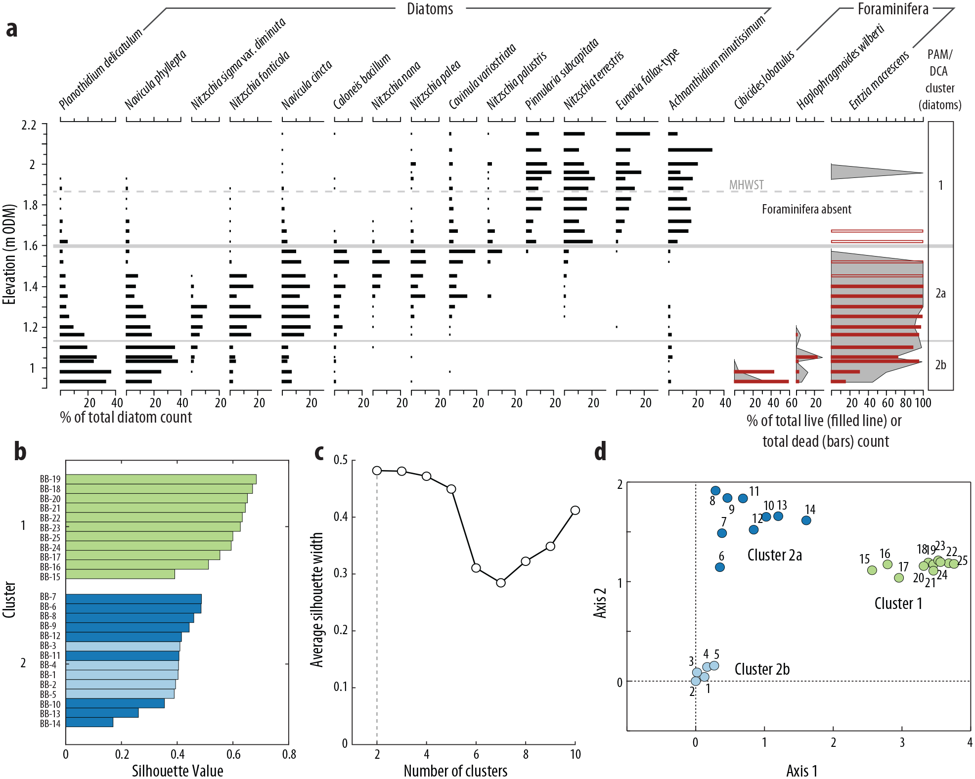
Modern microfossil assemblages from Bracky Bridge. (a) Vertical distribution of diatoms and foraminifera in the surface samples. Only common species exceeding 10% in one or more sample are shown. Dead foraminifera are shown as bars; living are shown with a filled line. Sample numbers increase from BB-1 at the lowest elevation to BB-25 at the highest. (b) Partitioning Around Medoids (PAM) algorithm silhouette plot showing the division of the diatom samples into two clusters; the two shades of blue in cluster 2 indicate the division observed in a Detrended Correspondence Analysis (DCA) sample plot (panel d). (c) Average PAM silhouette width with increasing number of clusters, demonstrating the optimum division into two. (d) DCA sample plot indicating division of the surface samples into three distinct clusters.

Pinnularia subcapitata, Nitzschia terrestris, Eunotia fallax-type and Achnanthidium minutissimum characterise cluster 1. A larger number of species exceed 10% in at least one sample in cluster 2a, with Navicula cincta and Nitzschia fonticola notably both exceeding 20%. Towards the lower elevations of this cluster, Planothidium delicatulum and Navicula phyllepta increase in abundance. These two species are dominant in the low marsh samples of cluster 2b, both exceeding 30% of the total assemblage. DCCA indicates that elevation explains 34% of the variance in the diatom data (Table 1).

Table 1.

Summary of the performance of the local Bracky Bridge and regional transfer functions.

Training set	No. of samples	% variance explained by elevation	Length of environmental gradient (DCCA, σ units)	Model type	Component/Deshrinking	Bootstrapped r²	RMSEP (SWLI)
Bracky Bridge	25	33.9	4.64	WA	Inverse	0.94	5.3
					Classical	0.94	5.2
				WA-TD	Inverse	0.94	5.6
					Classical	0.94	5.5
				WAPLS	1	0.94	5.6
					2	0.96	4.3
					3	0.96	4.1
Regional	323	2.6	4.07	WA	Inverse	0.73	16.9
					Classical	0.73	18.0
				WA-TD	Inverse	0.74	17.4
					Classical	0.74	17.8
				WAPLS	1	0.73	16.9
					2	0.78	15.9
					3	0.80	17.0
				LW-WAPLS	1	0.77	14.9
				LW-WAPLS	2*	0.84	12.6
					3	0.85	12.2

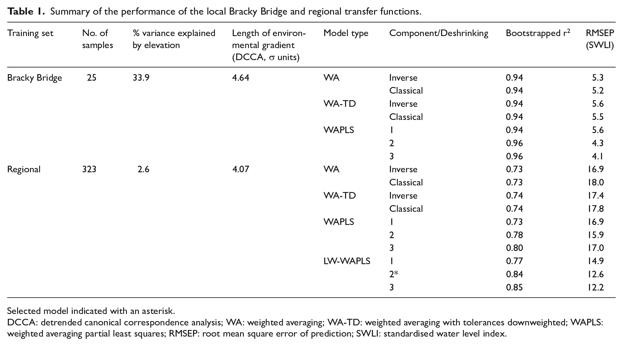
Selected model indicated with an asterisk.

DCCA: detrended canonical correspondence analysis; WA: weighted averaging; WA-TD: weighted averaging with tolerances downweighted; WAPLS: weighted averaging partial least squares; RMSEP: root mean square error of prediction; SWLI: standardised water level index.

Foraminifera

Of the 25 surface samples, 15 contained foraminifera, with only 11 providing dead counts in excess of 30 (Figure 2a; Supplemental Information S2, available online). We encountered a total of 17 different species in the dead assemblage, of which only three exceeded 10% in any one sample (Entzia macrescens, Cibicides lobatulus and Haplophragmoides wilberti). Apart from the lowermost two samples, the dead assemblages are dominated by E. macrescens (70–100%), with five monospecific samples. The two lowest elevation samples are more diverse, with C. lobatulus dominant (40–60%) alongside E. macrescens (15–30%), Elphidium williamsoni (7–9%) and 10 other rare species (0–5%).

Stained (assumed living) foraminifera occur in 14 samples, including an isolated individual at 1.96 m ODM, over 0.4 m higher than the next highest living specimen. The living assemblage includes 13 different species, of which only three – the same as those in the dead assemblage – exceed 10% of the total stained count in any one sample. The distribution of living foraminifera closely follows the dead distribution (Figure 2a).

Due to the small number of samples with sufficient total dead counts and the dominance of E. macrescens in most samples, we do not investigate clustering in the data and it is clear that the dataset is not suitable for the development of transfer functions to reconstruct palaeomarsh-surface elevations. Nevertheless, the modern data indicate that E. macrescens characterises vegetated tidal-marsh environments and this observation may be helpful for distinguishing such sediments.

Stratigraphy

A transect of 12 gouge cores maps the stratigraphy of the Bracky Bridge marsh (Figure 3). In the centre of the transect, we encountered a grey-brown peaty clay with Phragmites fragments overlying an impenetrable sand, gravel or rock substrate. A mid-brown herbaceous peat containing Phragmites, silty-clay, and occasionally sand overlies the peaty clay and is the uppermost layer in every core. At the northern end of the transect, the impenetrable substrate rises towards the surface and is overlain by ~0.3–0.5 m of organic sand and a thin surficial peat layer. The organic sand also extends as far south as core BB14 in a discrete layer approximately 0.1 m thick. Towards the southern end of the transect, around core BB13, sand and clay underlie ~1 m of surficial peat. At the base of the southernmost cores, BB10 to BB12, we recognise a layer of dark-brown to black well-humified peat overlying the basal substrate with an abrupt transition to uppermost unit of salt-marsh peat recorded elsewhere across the site. Here, the impenetrable substrate also rises towards the surface, with the overlying peat units reducing in thickness to less than 0.5 m.

Figure 3.

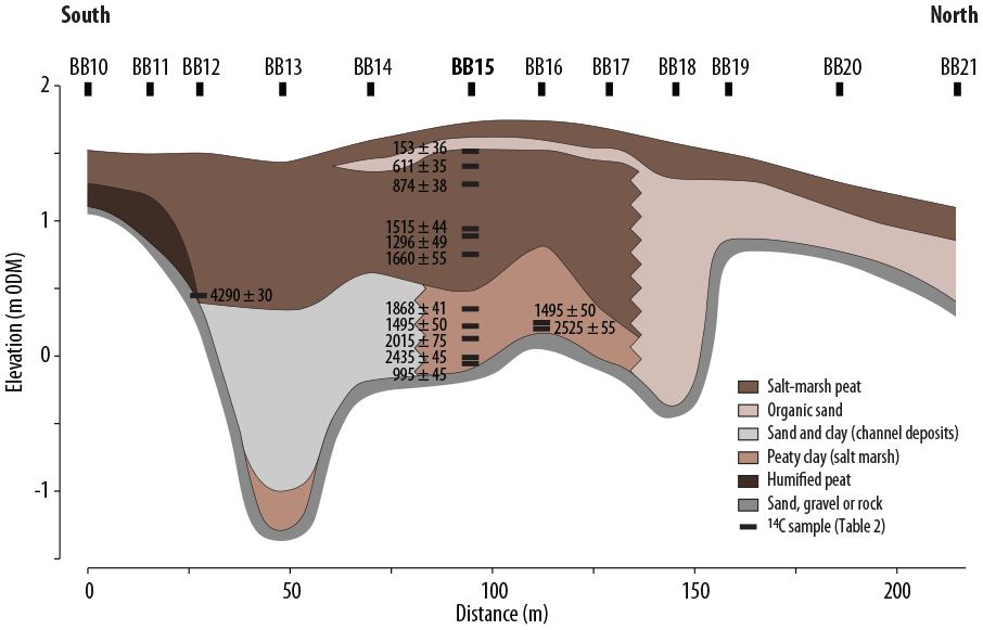
Stratigraphy of the Bracky Bridge coring transect. Core numbers are labelled, with the core chosen for detailed analysis in bold. Uncalibrated radiocarbon dates (Table 2) are indicated.

Table 2.

Radiocarbon samples from Bracky Bridge.

Core	Laboratory code	Core depth (cm)	Material	Radiocarbon age (years ± 1σ)	Calibrated age (years BP, 2σ, unmodelled)
BB15	AAR-8893	23	Detrital plant fragments	153 ± 36	0–285
	AAR-8894	33	Detrital plant fragments	611 ± 35	545–652
	AAR-8023	48	Detrital plant fragments	874 ± 38	688–905
	AAR-8024	80	Detrital plant fragments	1517 ± 44	1309–1516
	AAR-8025	84	Detrital plant fragments	1296 ± 49	1076–1300
	AAR-8026	99	Detrital plant fragments	1660 ± 55	1405–1698
	AAR-8027	139	Woody horizontal rootlet	1868 ± 41	1643–1884
	AAR-8028	153	Two pieces of detrital woody (bark) material	2265 ± 30	2156–2344
	AAR-8029	161	Yellow rootlet	2015 ± 75	1743–2283
	AAR-6865	175	Plant fragment	2435 ± 45	2353–2703
	AAR-6866	176	Plant fragment	995 ± 45	786–972
BB16	AAR-8061	149	Detrital plant fragments	1495 ± 50	1299–1515
BB16	AAR-8062	150	Bulk sediment	2525 ± 55	2374–2752
BB12	AAR-8063	110	Detrital Phragmites (?)	4290 ± 30	4825–4959

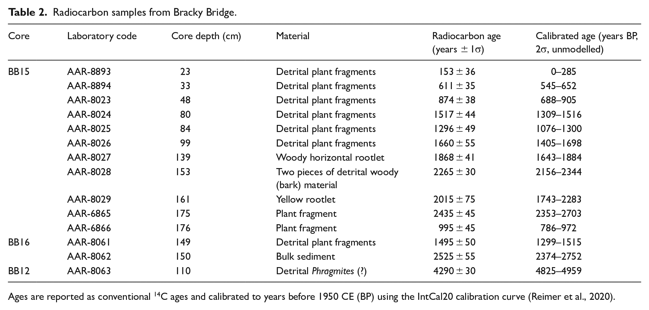
Ages are reported as conventional ¹⁴C ages and calibrated to years before 1950 CE (BP) using the IntCal20 calibration curve (Reimer et al., 2020).

We recovered a 1.82 m-long core from the centre of the transect, core BB15 (Figures 1d and 3). The surface elevation of this coring location is 1.77 m ODM. The core consists of 0.58 m of grey-brown peaty clay overlain by 1.24 m of mid-brown herbaceous peat. The upper peat layer includes a 0.10 m-thick organic sand layer at a depth of 0.10–0.20 m. We also recovered basal samples from locations BB12 and BB16 for radiocarbon dating and microfossil analyses. Core BB12 reached the impenetrable substrate at 1.16 m below the marsh surface (0.42 m ODM) and core BB16 at 1.50 m (0.26 m ODM). The basal sediments are dark-brown humified peat and peaty clay in BB12 and BB16 respectively.

Biostratigraphy

The 66 fossil samples from core BB15 yielded a total of 157 species of diatoms, including 14 that exceed 10% in at least one sample (Figure 4; Supplemental Information S3, available online). Of these 14 species, only N. cincta, A. minutissimum, C. bacillum, C. variostriata, Nitzschia palustris and N. terrestris also exceed 10% in the Bracky Bridge surface samples. Below 1.3 m core depth, diatom assemblages are dominated by the polyhalobian species Paralia sulcata (30–50%), alongside mesohalobian species including Navicula peregrina (4–25%) and Navicula digitoradiata (1–15%). From 1.30 m depth, Cosmioneis pusilla increases in abundance (10–35%) alongside P. sulcata (10–30%) and, from around 1.15 m depth, Diploneis interrupta (5–30%). After peaking at around 0.6 m depth, C. pusilla declines, with the interval between 0.5 m and 0.2 m depth seeing an increase in oligohalobian Pinnularia spp., predominantly an unknown species (5–60%). The uppermost 0.2 m are characterised by a diverse range of oligohalobian species, principally C. variostriata (1–50%) and C. bacillum (5–15%).

Figure 4.

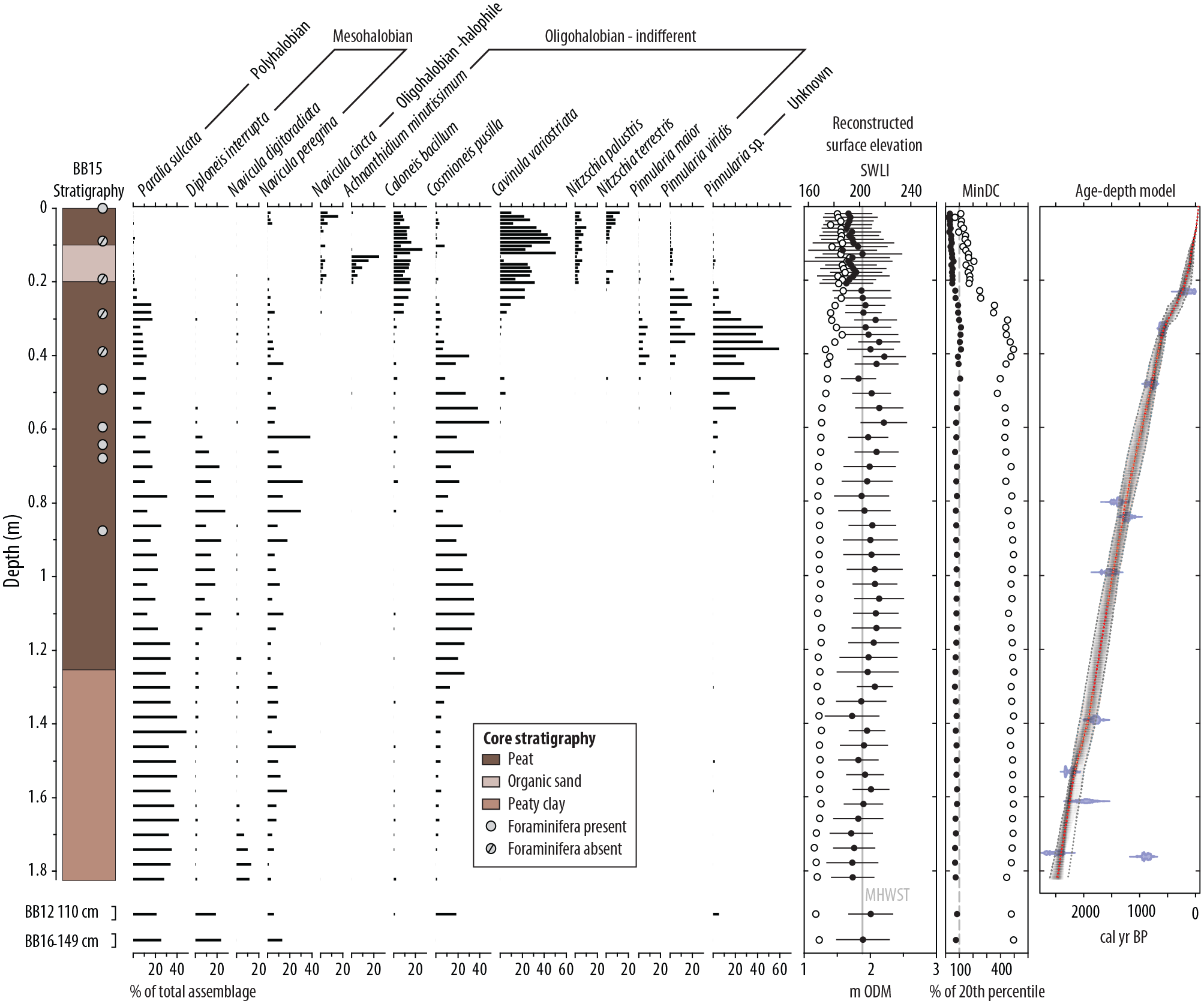
Fossil diatom assemblages (species exceeding 10% in at least one sample), palaeomarsh-surface elevation reconstructions, modern analogue technique minimum dissimilarity coefficients (MinDC), and age-depth model for core BB15. Surface elevation reconstructions are derived using the local Bracky Bridge transfer function (white circles, error bars not shown) and the regional transfer function (black circles, 2σ uncertainties). The distance to the closest modern analogue in the Bracky Bridge (white circles) and regional (black circles) training sets are shown as the percentage of the 20th percentile of the dissimilarities between the samples in the respective modern training sets, that is, a percentage of less than 100 (left of the dashed line) indicates a good or fair modern analogue. Age-depth model developed from ¹⁴C ages (blue probability distributions, Table 2) and ²¹⁰Pb data (Supplemental Information S5, available online) in the rplum package (Blaauw et al., 2022). Diatom assemblages from basal samples in cores BB12 and BB16 are also shown alongside corresponding surface elevation reconstructions and MinDC percentages.

Basal samples from 1.14 and 1.16 m core depth in BB12 yielded single specimens of D. interrupta, while a sample from 1.10 m provided 64 diatom valves, with D. interrupta, P. sulcata and Navicula pusilla the most common species. In core BB16, a sample at 1.49 m provided a full count, with P. sulcata, D. interrupta and N. peregrina the most common species.

Of the 10 samples analysed for foraminifera from the uppermost 0.90 m of core BB15, only samples from 0.59, 0.68 and 0.88 m depth contained greater than single-figure occurrences (Supplemental Information S4, available online). These samples contained up to 230 specimens of E. macrescens, the only species encountered in any of the fossil material. The basal samples from cores BB12 and BB16 were devoid of foraminifera.

Chronology

Eleven radiocarbon dates (Table 2) and 28 ²¹⁰Pb samples from the uppermost 0.3 m provide the chronology for core BB15 (Figure 4, Supplemental Information S5, available online). Additional ¹³⁷Cs data lack clear peaks that can be correlated with events of known ages and these data are, therefore, not used in age model development. The lack of ¹³⁷Cs peaks may reflect mobility in the profile (Foster et al., 2006), multiple possible sources (Foucher et al., 2021), or an insufficient sampling interval with respect to the sedimentation rate. The ²¹⁰Pb and ¹⁴C-based rplum age-depth model constrains the deposition of the sediments in core BB15 to the last ~2500 years, with age uncertainties (95% interval) for depths below 0.3 m averaging 230 years. The uppermost section of the core is better constrained due to the ²¹⁰Pb data, with age uncertainties decreasing from 160 years at 0.2 m (101–261 cal yr BP) to the known coring date at the surface. Modelled sedimentation rates average 0.07 cm yr⁻¹.

Three further radiocarbon dates constrain the timing of the deposition of the lowermost sediments in cores BB12 and BB16 (Table 2). In core BB16, plant macrofossils from 1.49 m depth give an age of 1299–1515 cal a BP, approximately 1000 years younger than a bulk sediment sample from 1.50 m depth. The younger age, coinciding with the diatom sample depth and relating to a sample type that is less susceptible to contamination by old carbon, is preferred. A plant macrofossil sample, likely a Phragmites fragment, from 6 cm above the base of core BB12 provides an age of 4825–4959 cal a BP.

Transfer function development and sea-level reconstruction

The dominance of one species and lack of zonation in the modern Bracky Bridge foraminiferal assemblages precludes their use as high-resolution sea-level indicators. The widespread distribution of E. macrescens mirrors the dominance of the sea rush J. maritimus and may similarly reflect low salinity conditions across the marsh resulting from the high annual rainfall and other unique characteristics of Irish salt-marshes (see Cott et al., 2012). The absence of foraminifera in many fossil samples further limits their utility at this site. Nevertheless, diatoms show excellent elevation-dependant zonation and sufficient fossil counts and are, therefore, highly suitable for quantitative RSL reconstructions.

Diatom transfer function performance

The 25 Bracky Bridge diatom samples provide the foundation for a local transfer function (Figure 5; Table 1). There is a strong relationship between observed and predicted elevations (r²_boot = 0.96 for the two component WAPLS model); however, underprediction of the elevations of the three uppermost samples results in a slight trend between observed and residual elevations (r² = 0.15).

Figure 5.

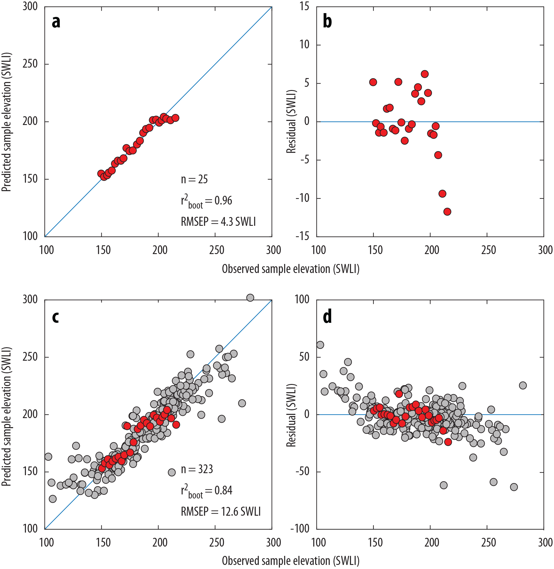
Performance of the local Bracky Bridge (panels (a and b)) and the regional (panels (c and d)) transfer function models. Panels (a and c) show observed elevation against transfer function-predicted elevation; panels (b and d) show residuals (predicted minus observed). Samples from Bracky Bridge are in red; samples from other sites are in grey.

While the local training set could be used to predict the elevation at which each fossil sample was deposited, we first assess whether the modern training set provides a sufficient range of assemblages to adequately represent the fossil material. Minimum dissimilarity coefficients indicate that the local training set fails to provide good or fair modern analogues for almost all of the fossil samples (Figure 4). Just two samples, both from within the uppermost 6 cm of core BB15, have fair modern analogues. The disparity between modern and fossil assemblages indicates that, despite the excellent performance, the local transfer function model may not provide accurate palaeomarsh-surface elevation reconstructions.

To address the lack of modern analogues, we combine the Bracky Bridge training set with published diatom distributions from 13 sites in western Scotland (Barlow et al., 2013; Shennan et al., 1995; Innes et al., 1996; Zong and Horton, 1999), south Wales (Gehrels et al., 2001) and southwestern England (Gehrels et al., 2001). The 323 samples in the combined ‘regional’ training set cover an elevation range of 102–281 SWLI, equivalent to 0.05–3.38 m ODM at Bracky Bridge or 273% of the local training set vertical range. This training set provides good analogues for 30% of the fossil samples and fair analogues for a further 63%. Just five samples (7 %), all between 0.32 and 0.47 m depth, continue to be poorly represented by the modern diatom assemblages. The change in the percentage of good and fair analogues between the local and combined models is the result of two factors. Between the surface of core BB15 and 0.25 m depth, surface samples from Bracky Bridge continue to provide the closest modern analogues, but the thresholds for good and fair analogues shift with the move to a larger and more diverse modern training set. In contrast, below 0.25 m, samples from other sites, principally the Erme (Figure 1a), provide more similar compositions.

Regional transfer functions based on the combined 14-site training set show a strong relationship between observed and predicted elevations (r²_boot = 0.84 for the two component LW-WAPLS model). Locally weighted models provide enhanced performance, with stronger relationships between observed and predicted elevations and smaller prediction uncertainties (Table 1; Figure 5). Nevertheless, there is a relationship between observed and residual elevations (r² = 0.23), with overprediction of surface elevations below 150 SWLI and underprediction above 225 SWLI. Within the 150–225 SWLI range, there is no relationship between observed and residual SWLI values (r² = 0.01). Caution must therefore be used when applying this transfer function and reconstructions outside of the central 150–225 SWLI range should be further interrogated.

Relative sea-level reconstruction

Calibration of the fossil diatom assemblages provides palaeomarsh-surface elevation reconstructions (Figure 4). Reconstructions using the local Bracky Bridge and the preferred regional transfer functions are within error in the uppermost 0.25 m of core BB15, but diverge below this depth. This divergence is due to the poor representation of the dominant fossil species, P. sulcata, D. interrupta, N. peregrina and Cosmioneis pusilla, in the Bracky Bridge surface samples (Figures 2 and 4). The reconstructions using the regional model are all within the central 150–225 SWLI range, varying between 184 and 218 SWLI, reducing the likelihood of systematic prediction biases.

We subtract the surface-elevation reconstructions from the field elevation of each sample to obtain the vertical position of palaeosea level and combine these with the modelled ages (see Chronology section) to reconstruct RSL change over time (Figure 6; Supplemental Information S6, available online). The reconstruction includes the basal and intercalated samples from core BB15 and the basal sample from core BB16. The humified peat at the base of core BB12 lacks diatom assemblages that would allow confident identification of intertidal deposition. While the sample from 1.10 m depth contains a small number of polyhalobian and mesohalobian specimens, we cannot rule out the possibility that these have been incorporated from the overlying salt-marsh peat into the underlying humified peat. As the radiocarbon sample lies at an unclear boundary between the two layers, we consider it a terrestrial limiting point rather than an index point.

Figure 6.

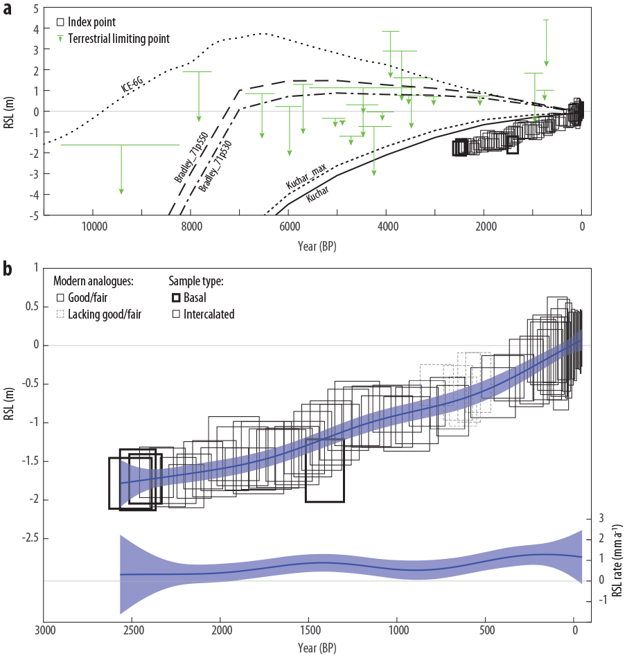
(a) The Bracky Bridge relative sea-level (RSL) reconstruction in the context of existing sea-level data (Shennan et al., 2018 and references therein), reinterpreted in the Discussion section. We plot relative sea-level predictions from five glacial isostatic adjustment models, two based on British-Irish Ice Sheet geomorphic extent data: Bradley_71p550 and Bradley_71p530 (Bradley et al., 2011, 2016; Shennan et al., 2018) and two based on a numerical ice-flow model: Kuchar and Kuchar_max (Kuchar et al., 2012), alongside the global ICE-6G(VM5a) model (Peltier et al., 2015). (b) Enlargement of the Late-Holocene Bracky Bridge reconstruction, with rates derived from an errors-in-variables integrated Gaussian process model (Cahill et al., 2016).

The earliest RSL constraint, a terrestrial limiting point derived from the basal sample from core BB12, places sea level below −0.5 m ODM at 4825–4959 cal yr BP (Figure 6). The basal and intercalated samples from core BB15 and the basal sample from core BB16 attest to continuously rising RSL from around −1.8 m ODM at 2500 cal yr BP to +0.1 m ODM at the end of the last millennium. The EIV-IGP model indicates the rate of RSL rise over the last 2500 years averaged 0.72 mm a⁻¹. Modest fluctuations reached maxima of 0.88 mm a⁻¹ (95% range 0.46–1.31 mm a⁻¹) in 1410 cal yr BP (540 CE) and 1.29 mm a⁻¹ (0.72–1.85 mm a⁻¹) in 150 cal yr BP (1800 CE) and a minimum of 0.52 mm a⁻¹ (0.05–0.99 mm a⁻¹) in 900 cal yr BP (1050 CE). As the core was collected in 2002, the Bracky Bridge reconstruction does not include any 21st century data points.

Discussion

The accumulation of a continuous near 2 -m-thick sequence of salt-marsh peat at Bracky Bridge necessitates a period of rising sea levels. Our reconstruction of continual RSL rise over the last 2500 years is consistent with this stratigraphy. Nevertheless, this reconstruction appears incompatible with previously published sea-level index points and proposed sea-level histories for the Donegal coastline that include a sea-level highstand and subsequent fall. In this section we attempt to reconcile this apparent contradiction through reinterpreting older sea-level data from the region and also consider possible sources of uncertainty in the Bracky Bridge record. Finally, we use the new RSL reconstruction as an empirical test for published GIA models.

Comparison with existing RSL data

Figure 6a displays the Bracky Bridge RSL reconstruction alongside sea-level data from the West Donegal region of the UK and Ireland sea-level database (Shennan et al., 2018). We assume that no correction is required to compare datasets tied to ODM (this study) and local mean sea level (Shennan et al., 2018). Shennan et al. (2018) interpret eight dates from Shaw (1985) and Shaw and Carter (1994) as index points, providing a sea-level history characterised by sea level reaching its present elevation around 4000 cal yr BP. Nevertheless, we note that none of these samples is accompanied by unequivocal evidence of intertidal deposition (e.g. intertidal microfossils such as foraminifera or diatoms in the dated units) and the samples could be alternatively and more conservatively interpreted as terrestrial limiting points, as we have in Figure 6a. While three samples from Ballyness and Clonmass do contain some pollen from salt-marsh plants (Shaw and Carter, 1994), indicating close proximity to salt-marsh environments, wind dispersal of key taxa such as Plantago maritima means a supratidal depositional elevation cannot be ruled out. Twelve further terrestrial limiting points from the West Donegal region relate to freshwater peats (Gaulin, 1983; Pearson, 1979; Shaw, 1985; Shaw and Carter, 1994; Smith and Pilcher, 1973; Telford, 1978).

Together, the 67 reconstructed positions of sea-level from Bracky Bridge and the 21 terrestrial limiting points (including the sample from core BB12), attest to sea levels rising to present, with no evidence for a Mid-Holocene highstand either close to or above present levels. Our reconstruction cannot rule out the possibility of a highstand; the distribution of limiting points could allow for sea level reaching present levels before 5000 cal yr BP. Nevertheless, the lack of index points before 2500 cal yr BP, combined with the limiting points constraining RSL to below −1 m ODM shortly after 5000 cal yr BP, and the subsequent rise from around −1.8 m ODM to present render a highstand of this elevation improbable and without a plausible driving mechanism.

The time periods covered by existing datasets and the main part of the reconstruction presented here are largely non-overlapping, with little previously published data from after 2500 cal yr BP. Two radiocarbon dates from Naran and Helgoland, approximately 10 km north of Bracky Bridge, do lie within this period (Shaw, 1985; Shaw and Carter, 1994). While the index points derived from these dates by Shennan et al. (2018) suggest higher sea levels than at Bracky Bridge, this inconsistency is resolved through our reinterpretation of the dated herbaceous peat layers as potentially freshwater rather than intertidal due to the lack of identified in situ salt-marsh microfossils in the samples (Figure 6a).

Compaction and tidal range as sources of uncertainty

Sediment compaction may result in post-depositional lowering of sea-level data (Brain, 2015; Brain et al., 2012). While the majority of the Bracky Bridge reconstruction is based on intercalated samples, which are more likely to be influenced by compaction, comparison of basal and intercalated samples suggests this process is unlikely to exert a major influence. Indeed, the basal sample from core BB16 suggests a sea-level position slightly lower than the contemporaneous intercalated samples from core BB15 (Figure 6b). Whilst not accounting for the magnitude of the reconstructed sea-level rise over the last 2500 years, differential compaction could, nevertheless, account for fluctuations in the modelled rates.

Changes in tidal range over time constitute another source of uncertainty in RSL reconstructions (Gehrels et al., 1995; Shennan and Horton, 2002). As our reconstruction relies on knowledge of the height of MHWST above MTL, an unrecognised increase in this range over time could be misinterpreted as a sea-level rise, even with no change in the mean level. Nevertheless, modelling studies suggest spring tidal ranges have remained consistent over the Late-Holocene in northwest Ireland (Neill et al., 2010), indicating that the Bracky Bridge reconstruction is unlikely to be strongly influenced by tidal-range changes.

Comparison with GIA models

The relative sea-level history from West Donegal presented here – in particular the lack of a Mid-Holocene highstand – provides an important empirical test for current and future GIA models. In Figure 6a, we compare the Bracky Bridge reconstruction and other published sea-level data with the change in RSL predicted by five published GIA models. As these models do not incorporate 20th and 21st century sea-level rise, we align the model predictions with the Bracky Bridge reconstruction for 1900 CE, ~−0.05 m OD. Two models (prefaced ‘Bradley’ in Figure 6a) with the same BIIS history, based on geomorphic extent data, but with different Earth rheologies, predict RSL reached 0.8–1.4 m above present between 6000 and 4000 cal yr BP (Bradley et al., 2011, 2016; Shennan et al., 2018). These models fail to plot below the terrestrial limiting points in the Mid-Holocene and predict a fall rather than a rise in the Late-Holocene. Predictions from ICE-6G(VM5a) (Peltier et al., 2015) indicate a higher and earlier highstand, reaching 3.75 m at 6500 cal yr BP, and an overall pattern that is again inconsistent with RSL constraints from West Donegal throughout the Holocene. Based on a numerical ice-flow model without the incorporation of geomorphic extent data, two models with varying ice thickness and extent, ‘Kuchar’ and ‘Kuchar_max’ in Figure 6a, provide contrasting predictions, with RSL rising monotonically from 11,000 cal yr BP to present (Kuchar et al., 2012). While none of the models fully predicts the timing and magnitude of the Late-Holocene relative sea-level rise reconstructed from Bracky Bridge, the Kuchar models most closely reflect the lack of an observed highstand and the continual rise to present.

Whilst sharing the same global ice-melt history, the glaciological model underpinning the Kuchar model predictions (Hubbard et al., 2009) suggests a thicker but less laterally extensive ice sheet than implied by the geomorphic extent data that are the foundation for the Bradley models (Brooks et al., 2008). Correspondingly greater isostatic uplift following deglaciation consequently results in subsequent barystatic rises not lifting RSL above present during the Holocene. Edwards et al. (2017) highlight that the Kuchar and Kuchar_max models are capable of predicting high Lateglacial sea levels in northern and western Ireland, while still adequately fitting Holocene sea-level data. Recently, extensive chronological data compiled through the BRITICE-CHRONO project has supported a thicker and also a more extensive ice sheet (Clark et al., 2022; Wilson et al., 2019). Whether the development of GIA models based on the BRITICE-CHRONO ice-sheet reconstruction improves the data-model misfit in West Donegal and other critical regions around the former BIIS (e.g. North Wales, Rushby et al., 2019) remains to be tested.

Conclusion

Holocene relative sea-level records from the coasts of northwestern Ireland and, in particular, western Donegal have the potential to provide a sensitive and discerning test for glacial isostatic adjustment models. Existing sea-level data from the region are, nevertheless, spatially and temporally limited, with uncertainties regarding the precise relationship between some indicators and contemporaneous sea levels. This paper has addressed this gap by providing – for the first time in Ireland – a sub-centennially resolved sea-level reconstruction from a continuous salt-marsh sediment sequence. Our reconstruction from Bracky Bridge is based on a quantitative microfossil proxy approach that first involves relating modern diatom assemblages to their preferred elevations with respect to tidal levels. We find that modern diatom assemblages from Bracky Bridge can provide transfer functions with excellent performance statistics, but dissimilarities between modern and fossil assemblages necessitate the development of a regional training set. A transfer function incorporating a total of 323 samples from 14 sites in western Scotland, southern Wales, southwestern England, and the study site in northwestern Ireland also performs well and provides a more suitable range of analogues for fossil samples.

The Bracky Bridge stratigraphy attests to relative sea-level rise over the last 2500 years and the combination of transfer function calibration and Bayesian age modelling reveals rates averaged 0.72 mm a⁻¹ over this period. A comparison of basal and intercalated samples indicates that this rise is unlikely to be related to sediment compaction. An apparent discrepancy with existing sea-level data from the region is resolved through a conservative reassessment of these discrete samples as terrestrial limiting rather than sea-level index points. The continual rise in relative sea level over the Late-Holocene and further constraints provided the terrestrial limiting points are likely incompatible with a Mid-Holocene sea-level highstand. The Late-Holocene sea-level rise is consistent with existing GIA models that incorporate a thick and extensive British-Irish Ice Sheet and provides a ready test for future modelling efforts.

Supplemental Material

sj-xlsx-1-hol-10.1177_09596836231169992 – Supplemental material for Holocene relative sea-level changes in northwest Ireland: An empirical test for glacial isostatic adjustment models

Supplemental material, sj-xlsx-1-hol-10.1177_09596836231169992 for Holocene relative sea-level changes in northwest Ireland: An empirical test for glacial isostatic adjustment models by Jason R Kirby, Ed Garrett and W Roland Gehrels in The Holocene

Supplemental Material

sj-xlsx-2-hol-10.1177_09596836231169992 – Supplemental material for Holocene relative sea-level changes in northwest Ireland: An empirical test for glacial isostatic adjustment models

Supplemental material, sj-xlsx-2-hol-10.1177_09596836231169992 for Holocene relative sea-level changes in northwest Ireland: An empirical test for glacial isostatic adjustment models by Jason R Kirby, Ed Garrett and W Roland Gehrels in The Holocene

Supplemental Material

sj-xlsx-3-hol-10.1177_09596836231169992 – Supplemental material for Holocene relative sea-level changes in northwest Ireland: An empirical test for glacial isostatic adjustment models

Supplemental material, sj-xlsx-3-hol-10.1177_09596836231169992 for Holocene relative sea-level changes in northwest Ireland: An empirical test for glacial isostatic adjustment models by Jason R Kirby, Ed Garrett and W Roland Gehrels in The Holocene

Supplemental Material

sj-xlsx-4-hol-10.1177_09596836231169992 – Supplemental material for Holocene relative sea-level changes in northwest Ireland: An empirical test for glacial isostatic adjustment models

Supplemental material, sj-xlsx-4-hol-10.1177_09596836231169992 for Holocene relative sea-level changes in northwest Ireland: An empirical test for glacial isostatic adjustment models by Jason R Kirby, Ed Garrett and W Roland Gehrels in The Holocene

Supplemental Material

sj-xlsx-5-hol-10.1177_09596836231169992 – Supplemental material for Holocene relative sea-level changes in northwest Ireland: An empirical test for glacial isostatic adjustment models

Supplemental material, sj-xlsx-5-hol-10.1177_09596836231169992 for Holocene relative sea-level changes in northwest Ireland: An empirical test for glacial isostatic adjustment models by Jason R Kirby, Ed Garrett and W Roland Gehrels in The Holocene

Supplemental Material

sj-xlsx-6-hol-10.1177_09596836231169992 – Supplemental material for Holocene relative sea-level changes in northwest Ireland: An empirical test for glacial isostatic adjustment models

Supplemental material, sj-xlsx-6-hol-10.1177_09596836231169992 for Holocene relative sea-level changes in northwest Ireland: An empirical test for glacial isostatic adjustment models by Jason R Kirby, Ed Garrett and W Roland Gehrels in The Holocene

Footnotes

Acknowledgements

We are grateful to Simon Newman for his assistance with field data collection and also for undertaking the foraminiferal analyses. We thank Ian Shennan, Sarah Woodroffe, and Natasha Barlow for providing access to diatom assemblage data and Graham Rush for his support with transfer function development. Sarah Bradley and Glenn Milne kindly provided the glacial isostatic adjustment model predictions. We thank Ann Kelly for assistance with laboratory work and the technical support provided in the School of Geography, Earth & Environmental Sciences at the University of Plymouth. Jan Heinemeier (University of Aarhus) and Tracy Shimmield (Dunstaffnage Laboratory, Oban, Scotland) conducted ¹⁴C and ²¹⁰Pb measurements, respectively. This work is a contribution to IGCP Project 725 ‘Forecasting Coastal Change’ and to PALSEA, a working group of the International Union for Quaternary Sciences (INQUA) and Past Global Changes (PAGES).

Funding

The author(s) disclosed receipt of the following financial support for the research, authorship, and/or publication of this article: This work was undertaken as part of HOLSMEER (Late-Holocene Shallow Marine Environments of EuRope), a European project funded by the ‘Energy, Environment and Sustainable Development’ programme of the Fifth Framework (contract EVK2-CT-2000-00060).

ORCID iDs

Jason R Kirby

Ed Garrett

Supplemental material

Supplemental material for this article is available online.

References

Aquino-López

Blaauw

Christen

, et al. (2018) Bayesian analysis of ²¹⁰ Pb dating. Journal of Agricultural Biological and Environmental Statistics 23(3): 317–333.

Aquino-López

Ruiz-Fernández

Blaauw

, et al. (2020) Comparing classical and Bayesian ²¹⁰Pb dating models in human-impacted aquatic environments. Quaternary Geochronology 60: 101106.

Barlow

NLM

Shennan

Long

, et al. (2013) Salt marshes as late Holocene tide gauges. Global and Planetary Change 106: 90–110.

Battarbee

Juggins

Gasse

, et al. (2001) European Diatom Database (EDDI). An Information System for Palaeoenvironmental Reconstruction. London: UCL Environmental Change Research Centre.

Birks

HJB

(1995) Quantitative palaeoenvironmental reconstructions. Quaternary. In: Maddy

Brew

(eds) Statistical Modelling of Quaternary Science Data. Cambridge: Quaternary Research Association, pp.161–254.

Birks

HJB

(2012) Overview of numerical methods in palaeolimnology. In: Birks

Lotter

Juggins

, et al. (eds) Tracking Environmental Change Using Lake Sediments. Dordrecht, Springer, pp.19–92.

Birks

HJB

Frey

Deevey

(1998) Numerical tools in palaeolimnology – Progress, potentialities, and problems. Journal of Paleolimnology 20: 307–332.

Blaauw

Christen

Aquino-Lopez

, et al. (2022) R Package rplum Version 0.2.2. https://CRAN.R-project.org/package=rplum

Bradley

Milne

Horton

, et al. (2016) Modelling sea level data from China and Malay-Thailand to estimate holocene ice-volume equivalent sea level change. Quaternary Science Reviews 137: 54–68.

10.

Bradley

Milne

Shennan

, et al. (2011) An improved glacial isostatic adjustment model for the British Isles. Journal of Quaternary Science 26(5): 541–552.

11.

Brain

(2015) Compaction. In: Shennan

Long

Horton

(eds) Handbook of Sea-level Research. Hoboken, NJ: Wiley Online Library, pp.452–469.

12.

Brain

Long

Woodroffe

, et al. (2012) Modelling the effects of sediment compaction on salt marsh reconstructions of recent sea-level rise. Earth and Planetary Science Letters 345-348: 180–193.

13.

Brooks

Bradley

Edwards

, et al. (2008) Postglacial relative sea-level observations from Ireland and their role in glacial rebound modelling. Journal of Quaternary Science 23(2): 175–192.

14.

Burningham

(2008) Contrasting geomorphic response to structural control: The Loughros estuaries, northwest Ireland. Geomorphology 97(3-4): 300–320.

15.

Burningham

Cooper

JAG

(2004) Morphology and historical evolution of north-east Atlantic coastal deposits: The west Donegal estuaries, north-west Ireland. Journal of Coastal Research Special Issue 41, 148–159.

16.

Cahill

Kemp

Horton

, et al. (2015) Modeling sea-level change using errors-in-variables integrated Gaussian processes. The Annals of Applied Statistics 9(2): 547–571.

17.

Cahill

Kemp

Horton

, et al. (2016) A Bayesian hierarchical model for reconstructing relative sea level: From raw data to rates of change. Climate of the Past 12(2): 525–542.

18.

Carter

RWG

Devoy

RJN

Shaw

(1989) Late-Holocene sea levels in Ireland. Journal of Quaternary Science 4(1): 7–24.

19.

Clark

Ely

Hindmarsh

RCA

, et al. (2022) Growth and retreat of the last British–Irish Ice Sheet, 31 000 to 15 000 years ago: the BRITICE-CHRONO reconstruction. Boreas. DOI: 10.1111/bor.12594

20.

Cott

Jansen

MAK

Chapman

(2012) Salt-marshes on peat substrate: Where blanket bogs encounter the marine environment. Journal of Coastal Research 28(3): 700–706.

21.

Curtis

TGF

Skeffington

MJS

(1998) The salt marshes of Ireland: An inventory and account of their geographical variation. Biology & Environment Proceedings of the Royal Irish Academy 98B: 87–104.

22.

Delaney

Devoy

(1995) Evidence from sites in western Ireland of late Holocene changes in coastal environments. Marine Geology 124(1-4): 273–287.

23.

Denys

(1991) A Check-List of the Diatoms in the Holocene Deposits of the Western Belgian Coastal Plain With a Survey of Their Apparent Ecological Requirements. Brussels: Belgian Geological Survey.

24.

Duffy

Devoy

RJN

(1998) Contemporary process controls on the evolution of sedimentary coasts under low to high energy regimes: Western Ireland. Geologie en Mijnbouw 77(3/4): 333–349.

25.

Edwards

Gehrels

Brooks

, et al. (2017) Resolving discrepancies between field and modelled relative sea-level data: Lessons from western Ireland. Journal of Quaternary Science 32(7): 957–975.

26.

Foster

IDL

Mighall

Proffitt

, et al. (2006) Post-depositional 137Cs mobility in the sediments of three shallow coastal lagoons, SW England. Journal of Paleolimnology 35(4): 881–895.

27.

Foucher

Chaboche

P-A

Sabatier

, et al. (2021) A worldwide meta-analysis (1977–2020) of sediment core dating using fallout radionuclides including ¹³⁷Csand ²¹⁰Pb_xs. Earth System Science Data 13(10): 4951–4966.

28.

Gallagher

Wheeler

Orford

(1996) An assessment of the heavy metal pollution of two tidal marshes on the north-west coast of Ireland. Biology & Environment Proceedings of the Royal Irish Academy 96B: 177–188.

29.

Gaulin

(1983) Analyse pollinique et detation par le 14C d’une tourbiere submergée de l’age de bronze dans le nord-Ouest de I’Lande (presqu’île de Termon. Dungloe, Comte Donegal). Comptes Rendus de l’Académie des Sciences Paris 296: 305–307.

30.

Gehrels

Belknap

Pearce

, et al. (1995) Modeling the contribution of M2 tidal amplification to the Holocene rise of mean high water in the Gulf of Maine and the Bay of Fundy. Marine Geology 124(1-4): 71–85.

31.

Gehrels

Roe

Charman

(2001) Foraminifera, testate amoebae and diatoms as sea-level indicators in UK saltmarshes: A quantitative multiproxy approach. Journal of Quaternary Science 16(3): 201–220.

32.

Geological Survey of Ireland (2022) Data and maps - noise. Available at: https://www.gsi.ie/en-ie/data-and-maps/Pages/default.aspx (accessed 21 September 2022).

33.

Hartley

(1996) An Atlas of British Diatoms. Bristol: Balogh Scientific Books.

34.

Hill

Gauch

(1980) Detrended correspondence analysis: An improved ordination technique. In: van der Maarel

(ed.) Classification and Ordination. Advances in Vegetation Science, vol. 2. Dordrecht: Springer, pp.47–58.

35.

Hocking

Garrett

Cisternas

(2017) Modern diatom assemblages from Chilean tidal marshes and their application for quantifying deformation during past great earthquakes. Journal of Quaternary Science 32(3): 396–415.

36.

Horton

Edwards

(2005) The application of local and regional transfer functions to the reconstruction of Holocene sea levels, north Norfolk, England. The Holocene 15(2): 216–228.

37.

Hubbard

Bradwell

Golledge

, et al. (2009) Dynamic cycles, ice streams and their impact on the extent, chronology and deglaciation of the British–Irish ice sheet. Quaternary Science Reviews 28(7-8): 758–776.

38.

Imbrie

Kipp

(1971) A new micropaleontological method for quantitative paleoclimatology: Application to a late Plestocene Caribbean core. In: Turekian

(ed.) Late Cenozoic Glacial Ages. New Haven, CT: Yale University Press, pp.71–181.

39.

Innes

Shennan

Twiddy

, et al. (1996) The contemporary diatom and pollen flora and foraminiferal fauna of Kentra Bay and Moss SSI, Lochaber. Scottish Natural Heritage Research Survey and Monitoring Report No. 31.

40.

Juggins

(2015) Rioja: Analysis of Quaternary Science Data. Newcastle upon Tyne: Newcastle University.

41.

Kaufman

Rousseeuw

(1990) Finding Groups in Data: An Introduction to Cluster Analysis. New York, NY: Wiley, pp.68–125.

42.

Kemp

Telford

Shennan

, et al. (2015) Transfer Functions. Handbook of Sea-Level Research. Chichester: Wiley-Blackwell, pp.470–499.

43.

Kemp

Wright

Cahill

(2020) Enough is enough, or more is more? Testing the influence of foraminiferal count size on reconstructions of paleo-marsh elevation. Journal of Foraminiferal Research 50(3): 266–278.

44.

Krammer

Lange-Bertalot

(1991) Süβwasserflora von Mitteleuropa. Bacillariophyceae. Stuttgart: Gustav Fischer Verlag.

45.

Krammer

Lange-Bertalot

(1997) Bacyllariopyceae: 1. Teil: Naviculaceae. Stuttgart: Gustav Fischer.

46.

Kuchar

Milne

Hubbard

, et al. (2012) Evaluation of a numerical model of the British-Irish ice sheet using relative sea-level data: Implications for the interpretation of trimline observations. Journal of Quaternary Science 27(6): 597–605.

47.

Met Éireann (2022) Rainfall Climate of Ireland. Available at: https://www.met.ie/climate/climate-of-ireland (accessed 21 September 2022).

48.

Murray

(1971) Living foraminiferids of tidal marshes; a review. Journal of Foraminiferal Research 1(4): 153–161.

49.

Murray

(1979) Recent benthic foraminiferids of the Celtic Sea. Journal of Foraminiferal Research 9(3): 193–209.

50.

Neill

(2020) Irish Coastal Wave and Water Level Modelling Study 2018: Phase 4 - Review of Mean Sea Level and OD Malin Relationship for the Coast of Ireland. Available at: https://s3-eu-west-1.amazonaws.com/docs.floodinfo.opw/floodinfo_docs/ICWWS-2018/Phase-4/IBE1505_ICWWS_Ph4_Rp04_F02.pdf (accessed 21 September 2022).

51.

Neill

Scourse

Uehara

(2010) Evolution of bed shear stress distribution over the northwest European shelf seas during the last 12,000 years. Ocean Dynamics 60(5): 1139–1156.

52.

Palmer

AJM

Abbott

(1986) Diatoms as indicators of sea-level change. In: van de Plassche

(ed.) Sea-Level Research. Norwich: Geobooks, pp.457–487.

53.

Pearson

(1979) Belfast radiocarbon dates IX. Radiocarbon 21(2): 274–290.

54.

Peltier

Argus

Drummond

(2015) Space geodesy constrains ice age terminal deglaciation: The global ICE-6G_C (VM5a) model. Journal of Geophysical Research Solid Earth 120(1): 450–487.

55.

Reimer

Austin

WEN

Bard

, et al. (2020) The IntCal20 Northern Hemisphere radiocarbon age calibration curve (0–55 cal kBP). Radiocarbon 62(4): 725–757.

56.

Rousseeuw

Kaufman

(1987) Clustering by means of medoids. In: Proceedings of the statistical data analysis based on the L1 norm conference, Neuchatel, Switzerland.

57.

Rushby

Richards

Gehrels

, et al. (2019) Testing the mid-Holocene relative sea-level highstand hypothesis in North Wales, UK. The Holocene 29(9): 1491–1502.

58.

Rush

McDarby

Edwards

, et al. (2021) Development of an intertidal foraminifera training set for the North Sea and an assessment of its application for Holocene sea-level reconstructions. Marine Micropaleontology 169: 102055.

59.

Scott

Hermelin

JOR

(1993) A device for precision splitting of micropaleontological samples in liquid suspension. Journal of Paleontology 67(1): 151–154.

60.

Scott

Medioli

(1980) Quantitative Studies of Marsh Foraminiferal Distributions in Nova Scotia: Implications for Sea Level Studies. Cushman Special Publications 17: 58.

61.

Shaw

(1985) Holocene coastal evolution, Co. Donegal, Ireland. Unpublished PhD Thesis, New University of Ulster.

62.

Shaw

Carter

RWG

(1994) Coastal peats from northwest Ireland: Implications for late-Holocene relative sea-level change and shoreline evolution. Boreas 23(1): 74–91.

63.

Sheehy Skeffington

Wymer

(1991) Irish Saltmarshes: An Outline Review. A Guide to the Sand Dunes of Ireland. Dublin: European Union for Dune Conservation and Coastal Management, pp.77–91.

64.

Shennan

(1982) Interpretation of Flandrian sea-level data from the Fenland, England. Proceedings of the Geologists Association 93(1): 53–63.

65.

Shennan

Bradley

Edwards

(2018) Relative sea-level changes and crustal movements in Britain and Ireland since the Last Glacial Maximum. Quaternary Science Reviews 188: 143–159.

66.

Shennan

Horton

(2002) Holocene land- and sea-level changes in Great Britain. Journal of Quaternary Science 17(5-6): 511–526.

67.

Shennan

Innés

Long

, et al. (1995) Holocene relative sea-level changes and coastal vegetation history at Kentra Moss, Argyll, northwest Scotland. Marine Geology 124(1-4): 43–59.

68.

Smith

Pilcher

(1973) Radiocarbon dates and vegetational history of the British Isles. New Phytologist 72(4): 903–914.

69.

Telford

(1978) Glenveagh Forest Park: The past and present vegetation. Unpublished PhD Thesis, National University of Ireland.

70.

Ter Braak

CJF

(1986) Canonical correspondence analysis: A new eigenvector technique for multivariate direct gradient analysis. Ecology 67(5): 1167–1179.

71.

Ter Braak

CJF

(1987) Unimodal Models to Relate Species to Environment. Wageningen: Wageningen University and Research.

72.

Ter Braak

CJF

Juggins

(1993) Weighted averaging partial least squares regression (WA-PLS): an improved method for reconstructing environmental variables from species assemblages. In: Twelfth international diatom symposium, pp.485–502. Dordrecht: Springer.

73.

Ter Braak

CJF

Smilauer

(2002) CANOCO Reference Manual and CanoDraw for Windows User’s Guide: Software for Canonical Community Ordination (Version 4.5). Ithaca NY, www.canoco.com (Microcomputer Power).

74.

Troels-Smith

(1955) Karakterisering af løse jordarter. Danmarks Geologiske Undersøgelse 3(10): 1–73.

75.

United Kingdom Hydrographic Office (2016) UK Admiralty Tide Tables. Taunton, United Kingdom Hydrographic Office.

76.

Van der Werff

Huls

(1958–1974) Diatoméenflora van Nederland, 8 parts. De Hoef, The Netherlands.

77.

Vos

de Wolf

(1993) Diatoms as a tool for reconstructing sedimentary environments in coastal wetlands; methodological aspects. Hydrobiologia 269-270(1): 285–296.

78.

Walton

(1955) Ecology of living benthonic foraminifera, Todos Santos bay, Baja California. Journal of Paleontology 29: 952–1018.

79.

Watcham

Shennan

Barlow

NLM

(2013) Scale considerations in using diatoms as indicators of sea-level change: Lessons from Alaska. Journal of Quaternary Science 28(2): 165–179.

80.

Wheeler

Oldfield

Orford

(1999) Depositional and post-depositional controls on magnetic signals from saltmarshes on the north-west coast of Ireland. Sedimentology 46(3): 545–558.

81.

Wilson

Ballantyne

Benetti

, et al. (2019) Deglaciation chronology of the Donegal Ice Centre, north-west Ireland. Journal of Quaternary Science 34(1): 16–28.

82.

Woodroffe

Long

(2010) Reconstructing recent relative sea-level changes in West Greenland: Local diatom-based transfer functions are superior to regional models. Quaternary International 221(1-2): 91–103.

83.

WoRMS Editorial Board (2022) World Register of Marine Species. Available at: https://www.marinespecies.org (accessed 21 September 2022).

84.

Zong

Horton

(1999) Diatom-based tidal-level transfer functions as an aid in reconstructing Quaternary history of sea-level movements in the UK. Journal of Quaternary Science 14(2): 153–167.

Supplementary Material

Please find the following supplemental material available below.

For Open Access articles published under a Creative Commons License, all supplemental material carries the same license as the article it is associated with.

For non-Open Access articles published, all supplemental material carries a non-exclusive license, and permission requests for re-use of supplemental material or any part of supplemental material shall be sent directly to the copyright owner as specified in the copyright notice associated with the article.

0.00 MB

0.12 MB

0.05 MB

0.08 MB

0.03 MB

0.04 MB

0.05 MB