Sage Journals: Discover world-class research

Abstract

Stratigraphic data from salt marshes provide accurate reconstructions of Holocene relative sea-level (RSL) change and necessary constraints to models of glacial isostatic adjustment (GIA), which is the dominant cause of Late-Holocene RSL rise along the U.S. mid-Atlantic coast. Here, we produce a new Mid- to Late-Holocene RSL record from a salt marsh bordering Great Bay in southern New Jersey using basal peats. We use a multi-proxy approach (foraminifera and geochemistry) to identify the indicative meaning of the basal peats and produce sea-level index points (SLIPs) that include a vertical uncertainty for tidal range change and sediment compaction and a temporal uncertainty based on high precision Accelerator Mass Spectrometry radiocarbon dating of salt-marsh plant macrofossils. The 14 basal SLIPs range from 1211 ± 56 years BP to 4414 ± 112 years BP, which we combine with published RSL data from southern New Jersey and use with a spatiotemporal statistical model to show that RSL rose 8.6 m at an average rate of 1.7 ± 0.1 mm/year (1σ) from 5000 years BP to present. We compare the RSL changes with an ensemble of 1D (laterally homogenous) and site-specific 3D (laterally heterogeneous) GIA models, which tend to overestimate the magnitude of RSL rise over the last 5000 years. The continued discrepancy between RSL data and GIA models highlights the importance of using a wide array of ice model and viscosity model parameters to more precisely fit site-specific RSL data along the U.S. mid-Atlantic coast.

Keywords

foraminifera glacial isostatic adjustment salt marsh sea-level change

Introduction

Proxy relative sea-level (RSL) reconstructions are crucial to decipher the processes causing sea-level change over various spatial and temporal scales prior to the instrumental record of sea level of the 19th and 20th centuries (e.g. Gehrels, 2000; Kemp et al., 2011; Kopp et al., 2016; Varekamp et al., 1992; Walker et al., 2021). Along the U.S. mid-Atlantic coast, such RSL reconstructions are provided by salt marsh sediments that accumulate with RSL rise over time, creating an archive of past change as salt marsh flora and fauna remain linked with the tidal frame (Morris et al., 2002; Psuty, 1986; Redfield, 1972). The U.S. mid-Atlantic coast is ideally located to assess the influence of glacial isostatic adjustment (GIA) – the dynamic response of the solid Earth to surface ice and water redistribution during ice age cycles (Clark et al., 1978). GIA is the dominant driver of Late-Holocene RSL rise along the U.S. mid-Atlantic coast, due to its proximity to the former margin of the Laurentide Ice Sheet (e.g. Engelhart et al., 2009; Gornitz and Seeber, 1990; Love et al., 2016; Roy and Peltier, 2015). As the Laurentide Ice Sheet retreated, the peripheral forebulge began to collapse, causing land subsidence, and Late-Holocene RSL rise (e.g. Clark et al., 1978; Davis and Mitrovica, 1996; Engelhart and Horton, 2012; Roy and Peltier, 2015). An accurate estimate of the contribution of GIA to Late-Holocene RSL is important for coastal adaptation, because in many regions subsidence is a principal reason for differences between regional and global-mean sea-level projections (e.g. Kopp et al., 2014; Love et al., 2016; Walker et al., 2021).

Accurate RSL reconstructions that include full consideration of vertical and temporal uncertainties are needed to validate GIA models (Khan et al., 2019). However, salt-marsh based RSL reconstructions can be modified by local processes such as sediment compaction (Horton and Shennan, 2009; Long et al., 2006; Törnqvist et al., 2004) and tidal range change (Gehrels et al., 1995; Hill et al., 2011; Shennan et al., 2003). Salt-marsh sediments are prone to sediment compaction, a process that occurs as sediment accumulates and becomes buried, reducing sediment volume and altering the geometry of the stratigraphic column (Allen, 2000; Horton and Shennan, 2009), resulting in an underestimation of past RSL (Allen, 2000; Edwards, 2006; Long et al., 2006). Changes in tidal range through time from factors such as changing bathymetry, coastlines, and shelf width can also affect RSL reconstructions, creating scatter among sea-level index points (SLIPs) (Gehrels et al., 1995; Hill et al., 2011; Horton et al., 2013; Shennan et al., 2000). Salt-marsh based RSL reconstructions that utilize basal peats (amorphous organic sediment overlying an incompressible substrate), as opposed to continuous cores, can provide valuable RSL data because they experience minimal sediment compaction (Horton and Shennan, 2009; Törnqvist et al., 2008). The benefits of using basal peats become especially significant when reconstructing RSL extending back to the Mid- to Late-Holocene, where the influence of sediment compaction in a long continuous core with thick overburden becomes increasingly pronounced.

Here, we produce a Mid- to Late-Holocene RSL reconstruction from a salt marsh in southern New Jersey. We use basal peat units and a multi-proxy approach of foraminifera and geochemistry (Kemp et al., 2012; Walker et al., 2020) to produce 14 SLIPs. Each SLIP includes an error for sediment compaction and tidal range change. Ages are produced through high precision Accelerator Mass Spectrometry (AMS) radiocarbon dating on salt-marsh plant macrofossils and calibrated using the IntCal20 dataset (Reimer et al., 2020). We combine our RSL data with published SLIPs (Horton et al., 2013) and a continuous 2500-year RSL record (Kemp et al., 2013) from southern New Jersey and use a spatiotemporal statistical RSL model (Ashe et al., 2019; Kopp et al., 2016) to assess magnitudes and rates of past RSL change. We compare the new RSL reconstruction to an ensemble of 1D (laterally homogenous; Peltier et al., 2015; Roy and Peltier, 2017) and site-specific 3D (laterally heterogeneous; Li and Wu, 2019; Li et al., 2018) GIA models, and the combined southern New Jersey dataset is compared to region-specific GIA models that consider the prediction uncertainties associated with 3D structure (Li et al., 2020).

Study area

The southern New Jersey coast is characterized by a barrier island and lagoon system adjacent to the Atlantic Ocean. The barrier island coastline is characteristic of trailing edges of passive continental margins and transgressive barriers (Inman and Nordstrom, 1971), which shelters the lagoon system in front of the geologically older Pleistocene mainland (Psuty, 1986). This region is a tectonically stable, passive continental margin with a coastal plain consisting of Cretaceous to Holocene unconsolidated sands, silts, clays, and gravels (Field and Duane, 1976). These coastal plain sediments have slowly subsided (<1 mm/year) since the Cretaceous due to thermal subsidence, sediment loading offshore, and compaction (Kominz et al., 1998) and have also likely been influenced by Cenozoic mantle dynamic topography (Schmelz et al., 2021).

The salt-marsh field study site is in Edwin B. Forsythe National Wildlife Refuge (referred to hereafter as Forsythe Refuge) on the west side of Great Bay in southern New Jersey (Figure 1a). Forsythe Refuge comprises and protects over 47,000 acres (190 km²) of a network of land and waters of the southern New Jersey coast, including over 35,000 acres (142 km²) of salt marshes (U.S. Fish & Wildlife Service, 2020). The southern New Jersey coast forms extensive gently sloping platforms of modern salt marshes with tidal channels (Ferland, 1990). The salt marsh vegetation comprises Spartina alterniflora (tall form) in low marsh areas along tidal creeks and Spartina patens and Distichlis spicata in high marsh areas, bordered by Phragmites australis adjacent to upland forest. The salt marshes of Forsythe Refuge were previously investigated by Kemp et al. (2013), who produced a RSL reconstruction over the last 2500 years in southern New Jersey using a foraminiferal-based transfer function.

Figure 1.

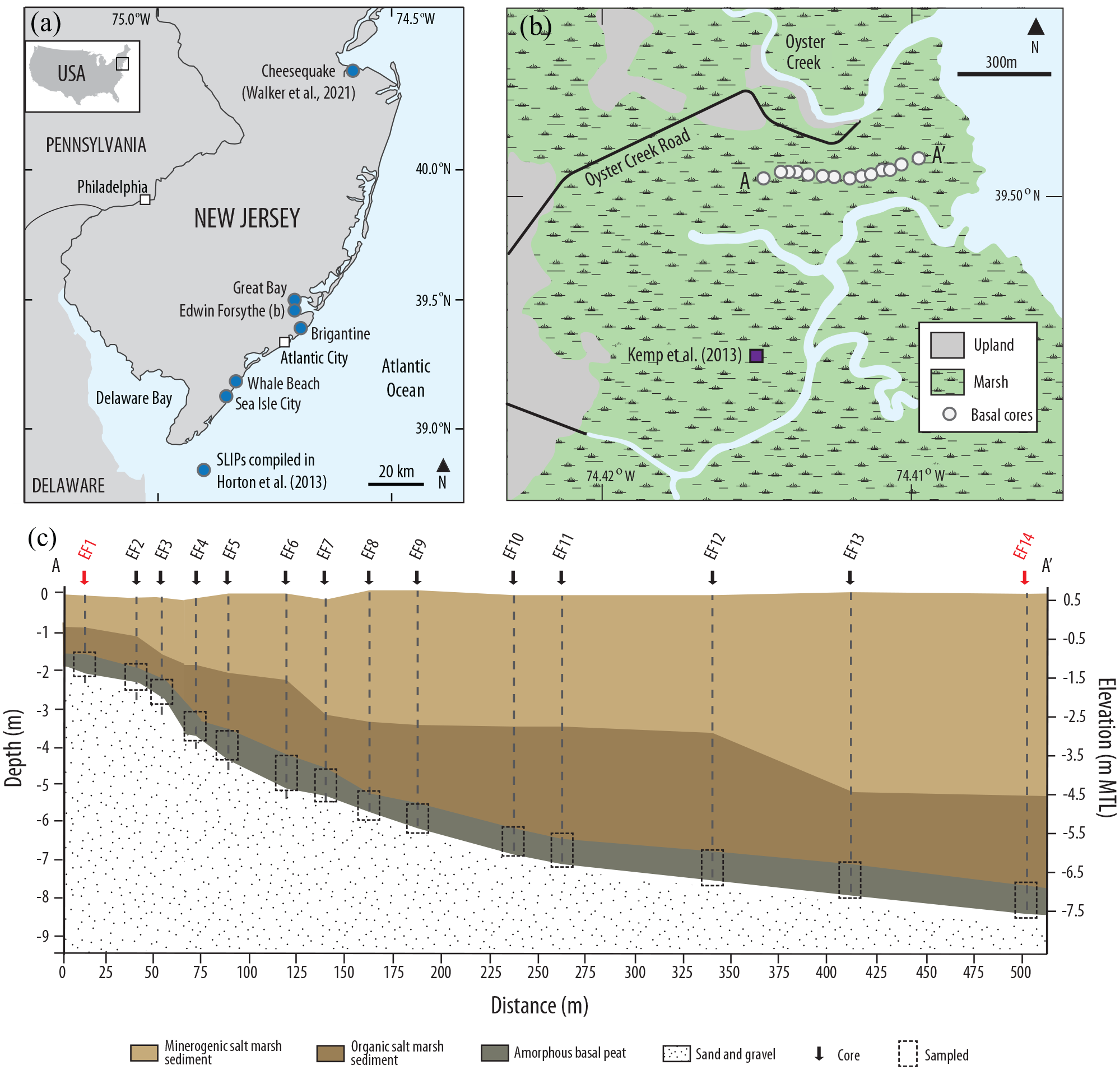
(a) Location of salt-marsh study site at Edwin B. Forsythe National Wildlife Refuge in southern New Jersey off of Great Bay. Also shown are site locations for continuous relative sea-level record from Cheesequake (Walker et al., 2021) and sea-level index points (SLIPs) compiled in Horton et al. (2013). (b) Salt-marsh study site showing basal core locations and core analyzed in Kemp et al. (2013). (c) Stratigraphy at salt-marsh study site with location of sediment cores and sampled basal unit of each core. The shortest (EF1) and longest (EF14) cores are highlighted in red.

The southern New Jersey coast has a semidiurnal, microtidal (range <2 m) regime, but varies between the ocean and lagoon side of the barriers. The tidal range at our field site, estimated by VDatum, is 1 m (Yang et al., 2008). Water exchange primarily occurs between the Atlantic Ocean and Little Egg Inlet leading into Great Bay (Chant et al., 2000).

Methods

Estimating paleomarsh elevation

We investigate the sediment stratigraphy along a transect of 14 core locations at Forsythe Refuge to retrieve basal peat sediments (Figure 1b). We describe the underlying lithostratigraphy according to the Troels-Smith (1955) classification of coastal sediments. The lower ~1 m of each of the 14 cores was collected so that the entire basal peat section is obtained, including the transition into the underlying incompressible substrate (Figure 1c). Each core is collected using a hand-driven Russian-type core to minimize compaction or contamination during sampling. We survey core top elevations using a temporary benchmark with real time kinematic (RTK) satellite navigation and a total station where elevations are referenced to the North American Vertical Datum (NAVD88). We use VDatum (Yang et al., 2008) to convert from orthometric to tidal datums.

We analyze basal cores for foraminifera and bulk-sediment carbon isotope composition (δ¹³C) in 1-cm slices at 5-cm spaced intervals to reconstruct RSL (Kemp et al., 2012, 2017a). Salt-marsh foraminifera are used as a proxy to reconstruct RSL, because their modern distributions exhibit vertical zonation with respect to tidal elevations (Gehrels, 1994; Horton and Edwards, 2006; Scott and Medioli, 1978). Stable carbon isotope geochemistry (reported as δ¹³C relative to VPDB) is used as a proxy for RSL because δ¹³C values in bulk marsh sediment represent the dominant vegetation type, and the transition between C₃ and C₄ dominated salt-marsh plant communities has been shown to act as the boundary for the mean higher high water (MHHW) tidal datum on the U.S. mid-Atlantic coast (Johnson et al., 2007; Kemp et al., 2012; Middelburg et al., 1997). Additional analytical details can be found in the Supplemental Materials.

We reconstruct the paleomarsh elevation (PME) of the samples from the basal cores using a Bayesian transfer function (BTF) (Cahill et al., 2016; Kemp et al., 2017a; Walker et al., 2020). The BTF utilizes a modern foraminiferal training set to quantify species assemblages’ relationship with tidal elevation, which is then applied to fossil assemblages to estimate a PME for each sample with a sample-specific uncertainty (Gehrels, 2000; Horton and Edwards, 2006; Horton et al., 1999). A secondary proxy, δ¹³C, is used to inform the prior distribution that is placed on elevation which can help reduce vertical uncertainty (Cahill et al., 2016; Kemp et al., 2017a). The BTF is developed using a New Jersey modern salt-marsh foraminiferal training set and δ¹³C that comprises 163 samples from 13 sites in southern New Jersey from Kemp et al. (2013) and 32 samples from northern New Jersey (Walker et al., 2021). We formally account for temporal and spatial variability of modern foraminifera distributions in the BTF by informing the prior distribution that describes the random variation of the individual foraminifera species using data from a monitoring study of modern foraminifera in southern New Jersey (Walker et al., 2020).

Due to differences in tidal range among sampling locations, we convert the tidal elevations into a standardized water level index (SWLI), following the approach of Horton et al. (1999), where a value of 100 corresponds to local mean tide level (MTL) and a value of 200 corresponds to local mean higher high water (MHHW).

Compaction

Sea-level reconstructions from basal peats are more resistant to the effects of sediment compaction since basal peats overlie an incompressible substrate (Shennan and Horton, 2002). However, only base of basal peat in direct contact with the incompressible substrate is completely unaffected by compaction (Törnqvist et al., 2008). We therefore use a geotechnical model (Brain et al., 2011, 2012, 2015) to estimate post-depositional lowering (PDL) resulting from sediment compaction within the basal peat cores. This approach has been used previously to correct salt-marsh RSL reconstructions for compaction along the mid-Atlantic coast (Kemp et al., 2017b). We collect modern marsh-surface core samples from Cape May Courthouse and Forsythe Refuge in southern New Jersey for laboratory geotechnical testing (Brain et al., 2015) (Supplemental Table 1). A full summary of the approach is provided in Brain (2015). We determine the compression behavior of the surface samples using automated oedometer testing (Head and Epps, 2011; Rees, 2014). We use the results to estimate parameter values for the Brain et al. (2011, 2012) compression framework that describes changes in volume in response to changes in vertical effective stress.

We measure organic content loss-on-ignition (LOI) and dry density at 2-cm intervals downcore for the entire length of the shortest (247 cm) core (EF1) and longest (863 cm) core (EF14) from the Forsythe Refuge transect. For LOI analysis, we dry the samples in an oven and ignite the samples in a muffle furnace following the methods of Head (2006). Using statistical relationships between compression model parameter values and measured LOI (Supplemental Table 2), we estimate compression properties downcore as model inputs. We then use the decompaction model to predict how the sediment throughout the core has been lowered from its depositional altitude. We compare measured and model-derived estimates of downcore dry density to assess the predictive capacity of the model (r²_adj = 0.75, p < 0.0001).

The model provides depth-specific estimates of PDL (±1 standard deviation) at 2 cm intervals downcore. For samples from the shortest (EF1) and longest (EF14) cores, the PDL estimate at the depth of the sample is included in the overall uncertainty assessments as a compaction error term. Due to the comparable stratigraphy along the basal core transect, for the remaining 12 cores, a compaction error term is added to each SLIP using the PDL estimates from the longest core, EF14, to represent the maximum potential PDL that each basal SLIP could have undergone.

Tidal range change

As tidal amplitudes are used in sea-level reconstructions, tidal changes due to astronomical forcing, ocean depth, density stratification, or coastal configuration (Griffiths and Hill, 2015) must be accounted for through time. For example, if tidal range was greater in the past, the PME would be greater and, consequently RSL would be lower, resulting in an underestimation of past sea-level change. We use a numerical paleotidal model following the methods of Horton et al. (2013) that predicts paleotidal data for New Jersey using a nested modeling approach (Hall et al., 2013; Hill et al., 2011), to include an error in the RSL data to account for changes in tidal amplitudes through time at Forsythe Refuge.

To calculate tidal amplitudes through time, a global tidal model (Griffiths and Peltier, 2008, 2009) is used to compute tidal amplitudes and phases on an 800 × 800 regular grid. A regional model (ADCIRC; Luettich and Westerink, 1991) allows for variable spatial resolution with nearshore resolution of 1–2 km to retain coastal embayment and estuary features. Hill et al. (2011) validated the model with approximately 250 NOAA tide-gages on the U.S. Atlantic and Gulf coasts and showed very good agreement between observations and model predictions. Depth changes from the ICE-5G GIA model of Peltier (2004) are used for paleobathymetries. The implication of choice of GIA model is minimized because of the microtidal ranges in New Jersey and, furthermore, we only include the tidal range change estimates as an error term in the RSL data rather than correcting the data (Hijma et al., 2015). Tidal amplitudes and phases from analysis of the regional model results are converted to tidal data using the harmonic constant datum method of Mofjeld et al. (2004).

An error is included in each SLIP to account for changes in tidal range from the time of sample deposition using the data from the paleotidal model. The model is run at 1000-year intervals, and data are extrapolated for our study site based on nearby model grid points. Following Hill et al. (2011), the percentage change in tidal range between present and the model runs is used to provide absolute values.

Reconstructing relative sea level

We reconstruct RSL from the basal cores of Forsythe Refuge as follows (Shennan and Horton, 2002):

{RSL}_{i} {= A}_{i}_{PME}_{i}

(1)

where A_i and PME_i are the altitude and paleomarsh elevation of the AMS radiocarbon sample i, respectively, and both values are expressed relative to MTL. A_i is established by subtracting the depth of each sample in the core from the surveyed core-top altitude. PME_i is estimated by the BTF with an associated 2σ uncertainty. We convert the PME estimates from the Bayesian transfer function from SWLI units back into meters relative to MTL specific to our study site.

Each sample also has additional errors specific to sea-level research (Engelhart and Horton, 2012; Shennan, 1986), with total error (2σ) for each sample given by (Shennan and Horton, 2002):

E_{i} = {(e_{2}^{1} + e_{2}^{2} + \dots + e_{n}^{2})}^{1 / 2}

(2)

These errors include a ± 0.05 m high precision surveying error (Gehrels, 1999; Shennan, 1986), a sample thickness error of ±half of sample thickness (Shennan, 1986), an angle of borehole error of ±1% overburden (Törnqvist et al., 2008), and a ± 0.01 error for compaction from the Russian hand corer (Shennan, 1986). In addition, we include the sediment compaction error term in our overall uncertainty estimate for each SLIP, which is estimated using the geotechnical model. Similarly, we include the tidal range change error term estimated using the paleotidal model.

We reconstruct RSL using the estimates of PME in combination with a sediment core chronology. For sample ages, we use radiocarbon dating by selecting plant macrofossils (stems and rhizomes) found in growth position from the base of the basal peat sequence in each core where foraminifera were still present. We chose plant macrofossils of stems in horizontal orientation in the core or rhizomes that included the junction to the above-ground stems to obtain reliable ages of paleo-marsh surfaces. The plant macrofossils are cleaned under a microscope to remove contaminant sediment particles and oven dried. The samples are submitted for AMS radiocarbon dating to the National Ocean Science Accelerator Mass Spectrometry (NOSAMS) facility and Beta Analytic. Reported radiocarbon ages and uncertainties (Table 1) are calibrated using the IntCal20 dataset (Reimer et al., 2020). We express the chronology in years before present (BP), so that all ages shown are calibrated years BP.

Table 1.

Reported radiocarbon ages and uncertainties from Forsythe Refuge basal cores with calibrated ages using the IntCal20 dataset (Reimer et al., 2020).

Core	Depth (cm)	Lab sample ID	Radiocarbon age (¹⁴C years)	Radiocarbon error (¹⁴C years)	Calibrated age (cal years. BP; 2 sigma range)
EF1	185	OS-135371	1310	15	1156–1267
EF2	235	OS-138362	1640	25	1436–1609
EF3	269	OS-138253	1770	20	1599–1707
EF4	298	OS-138251	1880	20	1717–1852
EF5	364	OS-137938	2240	20	2134–2313
EF6	411	OS-138074	2360	20	2295–2417
EF7	466	OS-137897	2850	20	2869–3050
EF8	514	OS-137786	2990	20	3053–3295
EF9	544	OS-137789	2960	25	3018–3226
EF10	582	OS-138359	3040	30	3156–3342
EF11	649	OS-135374	3320	25	3450–3607
EF12	732	OS-138164	3860	25	4161–4410
EF13	775	OS-137942	3950	25	4302–4526
EF14	811	Beta-516328	3800	30	4084–4289

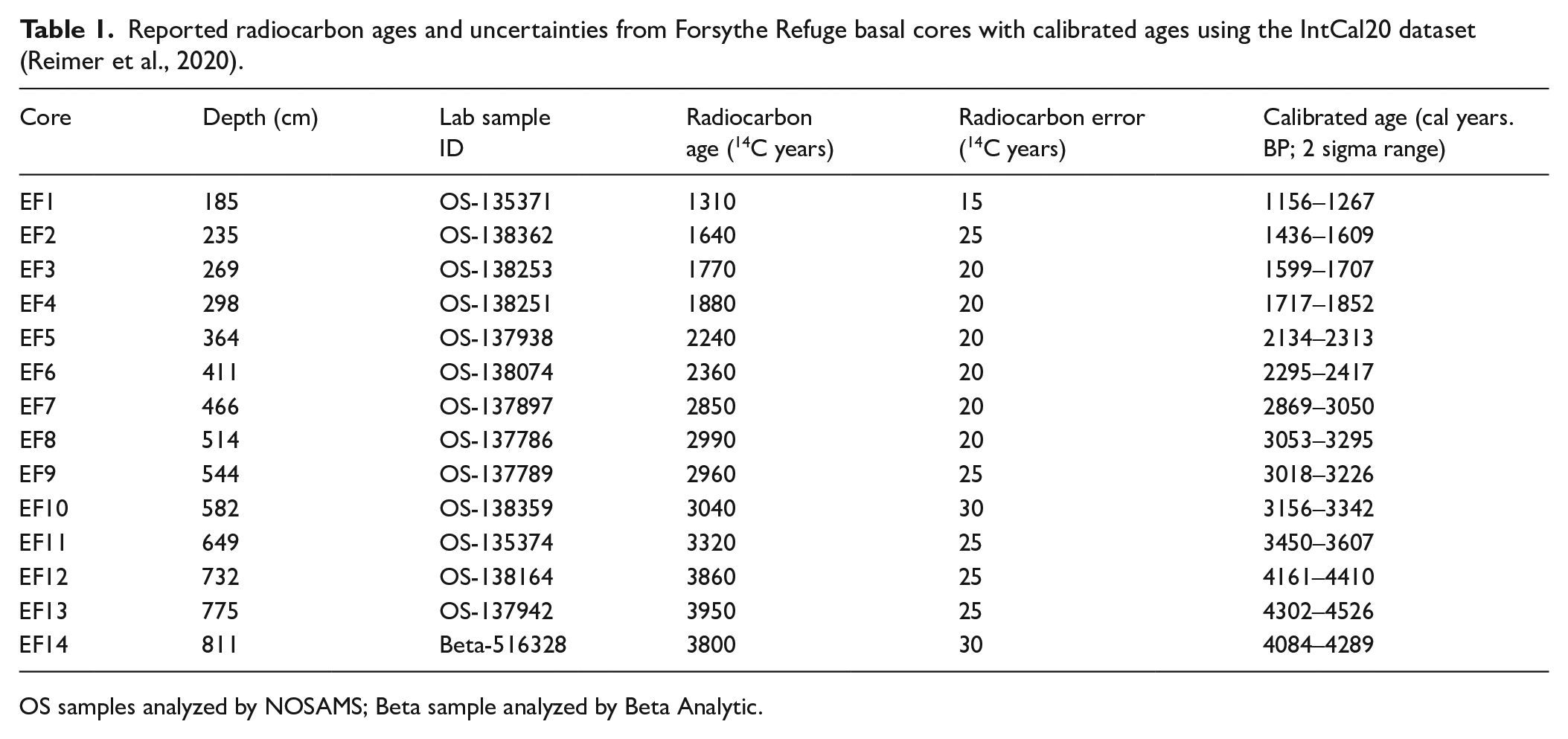
OS samples analyzed by NOSAMS; Beta sample analyzed by Beta Analytic.

We combine the basal peat record with a continuous RSL record from southern New Jersey (Kemp et al., 2013) for analysis of RSL change at Forsythe Refuge. To assess magnitudes and rates of RSL change in all of southern New Jersey, we produce a southern New Jersey sea-level database to use with a spatiotemporal empirical hierarchical model (Ashe et al., 2019; Kopp et al., 2016) (Supplemental Table 3). The southern New Jersey sea-level database includes: the basal peat record at Forsythe Refuge, the continuous RSL record from southern New Jersey (Kemp et al., 2013), and a compilation of published SLIPs from salt-marsh environments throughout New Jersey (Figure 1a) (Engelhart and Horton, 2012; Horton et al., 2013). To facilitate direct comparison with Forsythe Refuge, we include tidal range and sediment compaction effects as error terms rather than applying a correction as in Horton et al. (2013). Additional details of the spatiotemporal statistical model can be found in the Supplemental Materials.

GIA models

We compare the observed RSL changes over the last ~5000 years from the combined basal peat record at Forsythe Refuge and published RSL reconstruction from southern New Jersey (Kemp et al., 2013) with five individual GIA models, which includes two 1D models (ICE-6G_C (VM5a) (Argus et al., 2014; Peltier et al., 2015) and ICE-7G_NA (VM7) (Roy and Peltier, 2017)) and three 3D models from Li et al. (2018) and Li and Wu (2019).

The 3D viscosity models are labeled, for example VM_0.2_0.2_0.6_LHL, where the first digit indicates the background viscosity in the upper mantle (e.g. 0.2 × 10²¹ Pa s), the second digit represents the lateral heterogeneity scaling factor in the upper mantle ranging from 0 to 1 to determine the magnitude of lateral heterogeneity (e.g. 0.2), and the third digit represents the lateral heterogeneity scaling factor in the lower mantle (e.g. 0.6). Note that the background viscosity in the lower mantle is the same as that in VM5a. The final characters “LHL” indicate that the model includes the laterally heterogeneous lithosphere that is tuned in Li and Wu (2019). We only consider the upper mantle background viscosities of 0.2 × 10²¹, and 0.3 × 10²¹ Pa s as they have been shown to provide better fits with RSL data in North America (Kuchar et al., 2019; Li et al., 2018).

We evaluate the performance of each GIA model using a misfit χ-statistic (Li et al., 2018). The misfit χ-statistic compares the five individual GIA models with RSL changes over the last ~5000 years from: (1) the basal peat record at Forsythe Refuge and published RSL reconstruction from southern New Jersey (Kemp et al., 2013) and (2) RSL predictions at Forsythe Refuge from the spatiotemporal model, in which we treat the spatiotemporal model results as a series of data points in 500-year intervals covering the time period in which we have RSL data. The smaller the χ-statistic, the better the GIA predictions fit the Late-Holocene RSL data. The comparisons using the misfit χ-statistic exclude data in the last 200 years and redefine the RSL datum so that RSL is 0 at 150 BP. We do this to avoid bias in the misfit statistics because the GIA models do not account for the recent acceleration in RSL in the last ~200 years (Walker et al., 2022). Additional details of the GIA models and misfit χ-statistic can be found in the Supplemental Materials.

On a more regional scale, we also compare the southern New Jersey sea-level database with GIA models that consider the prediction uncertainties in North America from Li et al. (2020). The GIA model prediction uncertainties were assessed via a selection of models with different mantle viscosities (both 1D and 3D) and lithospheric, sublithospheric, and asthenospheric properties that provide the best fit with the deglacial RSL data, geodetic data, and gravity data in North America simultaneously. The selection of the best-fitting models provides the mean and 2σ uncertainties of RSL predictions (Li et al., 2020).

Relative sea-level reconstruction

Stratigraphy

The transect of 14 sediment cores covers a distance of ~500 m and ranges in depth from ~2 m at the inland end of the transect to ~9 m at the coastal edge of the marsh (Figure 1c). The stratigraphy across the transect has a 0.5 to 1-m basal unit of dark brown amorphous peat that thins away from the coast and overlies a gray incompressible sand and gravel. There is a very uniform gradient in the basal sand contact along the transect. Overlying the basal peat is ~1–3 m of dark brown organic-rich salt-marsh sediment that varies in thickness along the transect. The stratigraphy of the upper portion of the marsh is a brown relatively more minerogenic salt-marsh sediment which increases in thickness toward the coast from ~1 m in core EF1 to ~6 m in core EF14.

Paleomarsh elevation

We chose one basal sample in each of the 14 cores located at a depth where foraminifera counts were declining, before disappearing altogether as the basal incompressible sand was reached (Figure 2, Supplemental Figure 1). Paleomarsh elevation results for the shortest (EF1) and longest (EF14) sediment cores are displayed in Figure 2.

Figure 2.

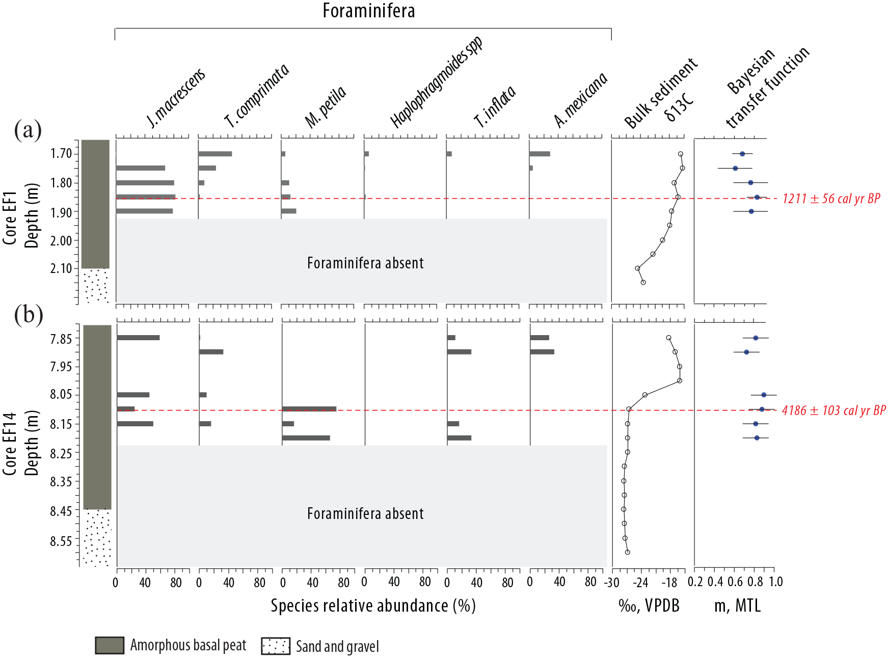
Foraminifera, δ¹³C, and Bayesian transfer function results for the (a) shortest (EF1) and (b) longest (EF14) basal sediment cores. Only the six most abundant foraminifera species are presented (Jadammina macrescens, Tiphotrocha comprimata, Milliammina petila, Haplophragmoides spp, Trochammina inflata, Arenoparella mexicana). Red dashed lines indicate depth of calibrated radiocarbon ages of sea-level index points. Sediment core data for other basal cores available in Supplemental Materials.

In core EF1, the upper portion of the basal peat unit is dominated by Tiphotrocha comprimata and Arenoparella mexicana (~75% of the assemblage together), but transitions to an assemblage dominated by Jadammina macrescens and Miliammina petila (up to 100% of the assemblage together) with depth until the foraminifera become absent altogether below 190 cm (Figure 2a). Our basal sample is at a depth of 185 cm, where J. macrescens and M. petila are the dominant species. The δ¹³C at the top of the basal core is −15.7‰ which becomes steadily more depleted with depth to −23.4‰ at the base.

In core EF14, the upper portion of the basal peat unit has a mixed assemblage of J. macrescens, T. comprimata, Trochammina inflata, and A. mexicana. J. macrescens and M. petila become the dominant species (~70–100% of the assemblage together) with depth until the foraminifera become absent below 820 cm. Our basal sample is at a depth of 811 cm. The δ¹³C in the upper portion of the basal core ranges from −16.0‰ to −18.3‰ before rapidly becoming more depleted, ranging from −23.2‰ to −27.6‰ through the rest of the core.

Similar foraminifera assemblage trends were found in the other basal cores, where the upper portion includes include greater abundances of species such as A. mexicana or T. inflata but are less prevalent with depth. The most consistent trend among the basal cores was that J. macrescens and/or M. petila are dominant species at the lowest depths where foraminifera were present and are also two of the most dominant species in our samples. The dominant foraminifera species in our basal samples are indicative of a high salt marsh environment. In New Jersey, high marsh assemblages have been dominated by J. macrescens and T. comprimata, and Haplophragmoides spp. has been found to be a dominant species in high marsh and transitional high marsh-upland environments, often above MHHW (Kemp et al., 2012, 2013). Kemp et al. (2013) also found high abundances of M. petila in the lower portion of a core from Forsythe Refuge. The δ¹³C values in other basal cores also become more depleted with depth. The δ¹³C values at the depth of each SLIP or the nearest depth where δ¹³C was measured range from −16.2‰ to −26.6‰.

The reconstructed PME estimates from the Bayesian transfer function for all of the basal samples range from 0.55 m MTL to 0.94 m MTL with sample-specific uncertainties (2σ) ranging from 0.21 to 0.61 m (Figure 2, Supplemental Figure 1). For example, in core EF1, the basal sample has a PME of 0.83 ± 0.26 m MTL and in core EF14, the basal sample has a PME of 0.89 ± 0.24 m MTL.

Compaction

Compaction model results for the shortest (EF1) and longest (EF14) sediment cores are displayed in Figure 3. Measured LOI for core EF1 varies from ~50% at the top of the core to ~2% at the base of the core in the basal sand unit (Figure 3a). The mean LOI in the lower ~0.5 m of the core is ~4%, and then increases to an average of 27% in the upper 2 m. Core EF14 has a lower LOI % at the top of the core (~15%), but a slightly higher LOI % at the base of 7% compared to core EF1 (Figure 3b). LOI is variable in the upper ~8.3 m, ranging from 7% to 49%, before decreasing to the base. Measured dry density for core EF1 varies from ~0.2 g/cm³ at the top of the core to ~2.0 g/cm³ at the base of the core (Figure 3a). Similar to LOI, the mean dry density in the lower ~0.5 m of the core is ~1.6 g/cm³, and then markedly decreases to a mean of 0.3 g/cm³ in the upper 2 m of the core. Measured dry density for core EF14 varies from ~0.4 g/cm³ at the top of the core to ~1.4 g/cm³ at the base of the core (Figure 3b). Similar to LOI, the dry density varies in the upper ~8.3 m from 0.2 to 1.0 g/cm³, and then rapidly increases to the base.

Figure 3.

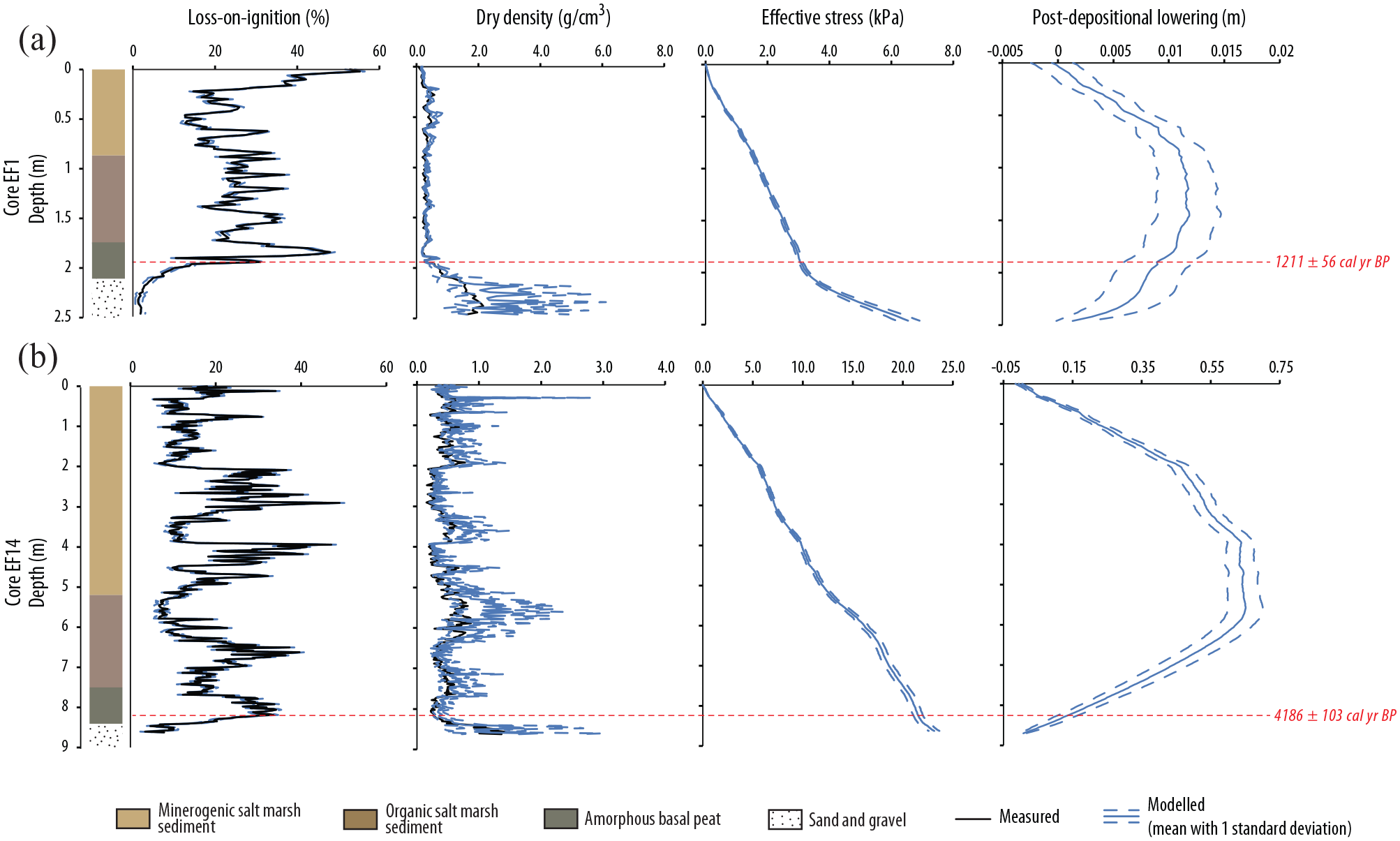
Estimation of post-depositional lowering caused by sediment compaction. Measured and modeled loss-on-ignition and dry density and modeled effective stress and post-depositional lowering predicted by the geotechnical model for the (a) shortest (EF1) and (b) longest (EF14) sediment cores. Red dashed lines indicate depth of calibrated radiocarbon ages of sea-level index points. Note different axis scales between cores.

The effective stress predicted by the geotechnical model in core EF1 increases with depth to 3.3 kPa at 2 m depth before increasing more rapidly with depth in the lower 0.5 m of the core, to 6.5 kPa at the base (Figure 3a). Core EF14 has a continually increasing effective stress depth profile, reaching a maximum of ~23 kPa at the base of the core (Figure 3b). PDL estimated by the model for core EF1 is 0 m at the surface, increases to a maximum PDL of ~0.01 m in the middle of the core around 1.3 m depth, and then decreases back to 0 m at the base of the core. The PDL estimate for core EF14 is also 0 m at the surface, but then increases to a much larger maximum PDL of ~0.65 m in the middle of the core around 5.5 m depth, before decreasing back to 0 m at the base of the core. The greater PDL in core EF14 clearly exhibits the influence of sediment compaction within deep sequences of salt-marsh sediment, which could influence RSL reconstructed from continuous sequences of sediment.

The estimated PDL for the sample at 1.85 m depth in core EF1 is 0.01 ± 0.01 m, compared to the sample in core EF14 at a depth of 8.11 m which has a PDL estimate of 0.16 ± 0.06 m. Each of these PDL estimates is included as a compaction error term in the overall assessment of uncertainty. To account for sediment compaction of the SLIPs in the other 12 cores in which we did not estimate PDL with the geotechnical model, we include the PDL estimate from core EF14 as a compaction error term in each PME estimate, as this value is the largest magnitude PDL we would expect in any shorter core.

Tidal range change

The present-day and modeled tidal range for each SLIP during the Late-Holocene is displayed in Figure 4. The Great Diurnal Range (GT) is the difference between mean higher high water and mean lower low water (NOAA, 2000) and in New Jersey, the GT is microtidal (<2 m). Paleotidal modeling indicates that the GT was 24% greater in the past, reaching ~0.24 m higher at 5000 years BP compared to present (Figure 4). The SLIP from core EF1 has the smallest increase in tidal range of 0.05 m at ~1200 years BP compared to the SLIP in core EF14 which has an increase in tidal range of 0.20 m at ~4200 years BP. An error is included for each of the 14 SLIPs to account for differences in tidal range at the time of sample deposition.

Figure 4.

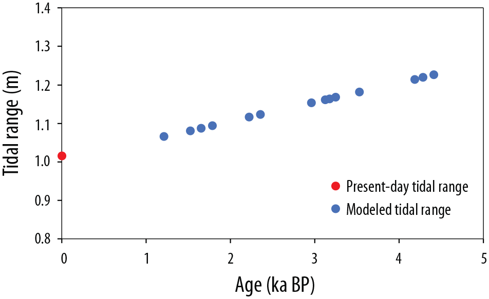
Present-day and modeled tidal range for each sea-level index point during the Late-Holocene predicted from the paleotidal model (Hall et al., 2013; Hill et al., 2011).

Sea-level index points

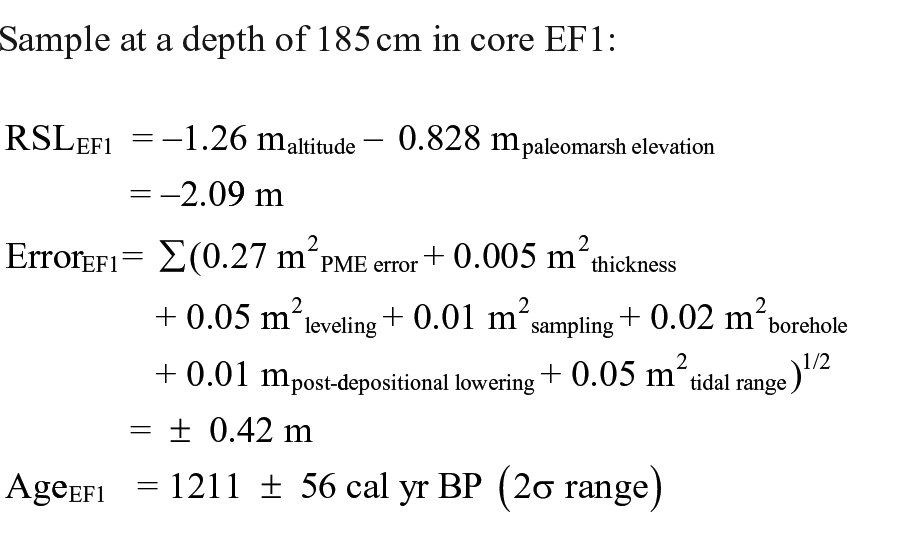
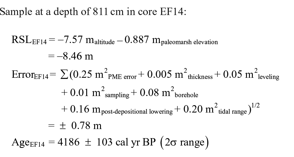
We produce 14 basal SLIPs from Forsythe Refuge over the Mid- to Late-Holocene (Figure 5, Table 1). The basal SLIPs range from 1211 ± 56 years BP at a sample elevation of −1.26 m MTL to 4414 ± 112 years BP at a sample elevation of −7.18 m MTL. The calculation of RSL and age, including errors, was as follows (using examples from cores EF1 and EF14):

Figure 5.

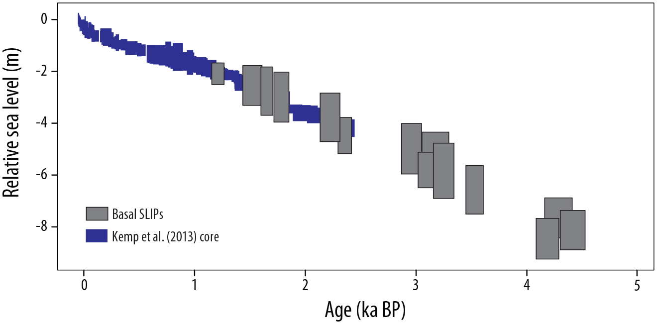
Basal sea-level index points (SLIPs) from Forsythe Refuge site in southern New Jersey plotted as boxes with 2σ vertical and calibrated age errors and continuous relative sea-level record from Kemp et al. (2013).

\begin{array}{l} Sample at a depth of 185 cm in core EF 1 : {RSL}_{EF 1} =_1.26 m_{altitude}_0.828 m_{paleomarsh elevation} \\ =_2.09 m \\ \begin{array}{l} {Error}_{EF 1} = \sum (0.27 m_{PME error}^{2} + 0.005 m_{thickness}^{2} \\ + 0.05 m_{leveling}^{2} + 0.01 m_{sampling}^{2} + 0.02 m_{borehole}^{2} \end{array} \\ + 0.01 m_{post - depositional lowering} + 0.05 m_{tidal range}^{2})^{1 / 2} \\ = \pm 0.42 m \\ {Age}_{EF 1} = 1211 \pm 56 cal yr BP (2 σ range) \end{array}

\begin{array}{l} Sample at a depth of 811 cm in core EF 14 : {RSL}_{EF 14} =_7.57 m_{altitude}_0.887 m_{paleomarsh elevation} \\ =_8.46 m \\ \begin{array}{l} {Error}_{EF 14} = \sum (0.25 m_{PME error}^{2} + 0.005 m_{thickness}^{2} + 0.05 m_{leveling}^{2} \\ + 0.01 m_{sampling}^{2} + 0.08 m_{borehole}^{2} \end{array} \\ + 0.16 m_{post - depositional lowering} + 0.20 m_{tidal range}^{2})^{1 / 2} \\ = \pm 0.78 m \\ {Age}_{EF 14} = 4186 \pm 103 cal yr BP (2 σ range) \end{array}

The basal SLIPs overlap with the continuous cores from Kemp et al. (2013), and the combined RSL record shows continuously rising RSL from 4500 years BP to present (Figure 5). The results from the spatiotemporal model for Forsythe Refuge show that RSL rose by an approximate magnitude of 8.6 m at an average rate of 1.7 ± 0.1 mm/year (1σ) from 5000 years BP to present. RSL was ~7 m below present at 4000 years BP and ~3.5 m below present at 2000 years BP. Over the last 200 years, RSL rose ~0.7 m at a rate of rise of 3.3 ± 0.4 mm/year (Figure 6).

Figure 6.

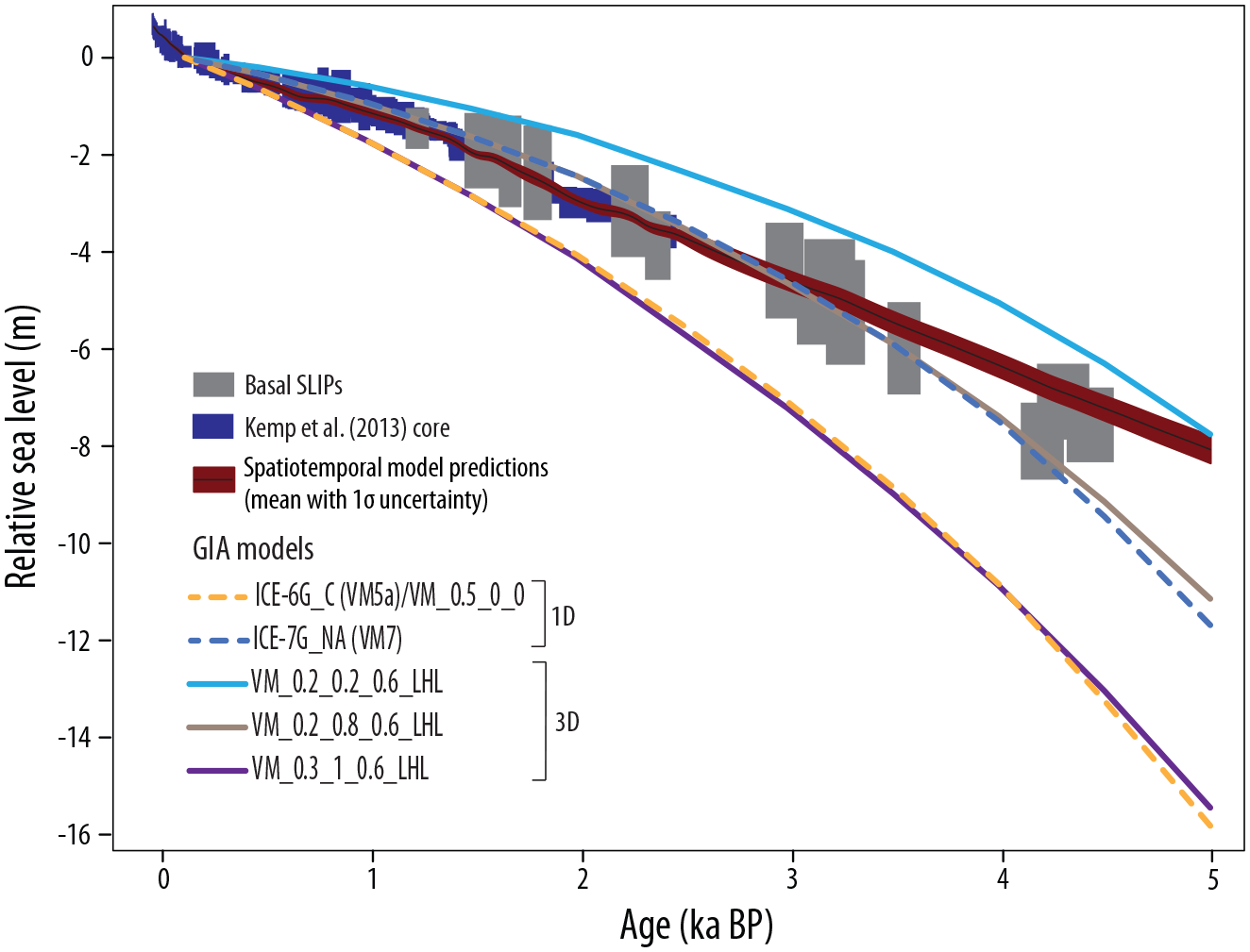
Comparison of basal sea-level index points (SLIPs) from Forsythe Refuge site in southern New Jersey and continuous relative sea-level record from Kemp et al. (2013) with five GIA model predictions (two 1D models and three 3D models) over the last 5000 years BP. Spatiotemporal model predictions are also shown with the mean and 1σ uncertainty. The zero sea-level datum is at 150 years BP.

Discussion

New Jersey relative sea level

RSL has risen along the entire U.S. Atlantic coast during the Late-Holocene at differing rates due to spatially variable GIA-induced subsidence and other regional processes (e.g. oceanographic effects). Late-Holocene RSL rise in New Jersey has been dominated by GIA due to New Jersey’s close proximity to the former Laurentide Ice Sheet margin (Engelhart et al., 2009; Love et al., 2016; Roy and Peltier, 2015). The Forsythe Refuge basal peat record and southern New Jersey database show continuously rising sea level through the Late-Holocene. Previous studies from New Jersey also show continuous RSL rise of similar magnitude (~8 m) during the last 4000 years (Bloom, 1967; Daddario, 1961; Horton et al., 2013; Miller et al., 2009; Psuty, 1986). For example, Psuty (1986) examined sea-level trends using radiocarbon dates from sediment cores around Great Bay and elsewhere in New Jersey and found rising RSL from at least 7700 years BP to present, with a rapid rate of rise beginning before 7000 years BP, followed by a decrease in rates 2500 to 2000 years BP. We found an average rate of rise of 1.7 ± 0.1 mm/year in southern New Jersey over the last 5000 years, which is also comparable to previous findings over the Mid- to Late-Holocene. Miller et al. (2009) reconstructed RSL in New Jersey over the last 5000 years and found a similar relatively constant rise of 1.7–1.9 mm/year from −5000 to 500 years BP, while Miller et al. (2013) found a rise of 1.6 ± 0.1 mm/year from 2200 to 1200 years BP. After accounting for compaction and change in tidal range, Horton et al. (2013) found that RSL in New Jersey rose at an average rate of 4 mm/year from 10,000 to 6000 years BP, 2 mm/year from 6000 to 2000 years BP, and 1.3 ± 0.1 mm/year from 2000 to 50 years BP. Kemp et al. (2013) reconstructed RSL over the last 2500 years in southern New Jersey and, after correcting for land-level change (1.4 mm/year), found four multi-centennial sea-level trends using change point analysis: fall at 0.1 ± 0.1 mm/year from 2450 to 1700 years BP, rise at 0.6 ± 0.2 mm/year from 1700 to 1217 years BP, fall at 0.1 ± 0.1 mm/year from 1217 to 100 years BP, and rise at 3.1 ± 0.3 mm/year since 100 years BP. In northern New Jersey, Walker et al. (2021) found continuously rising RSL from 1000 years BP to present at an average rate of 1.5 ± 0.2 mm/year (2σ).

While using SLIPs from basal peat samples minimizes the potential errors due to processes such as sediment compaction, this method limits analysis of the relative roles of driving processes and changing rates through time due to the lower frequency of data. Methods of sea-level reconstruction using continuous cores and age depth models produce continuous RSL data to enable more detailed analysis of centennial-scale trends and their drivers (Gehrels et al., 2020; Kemp et al., 2018; Walker et al., 2021). However, basal peats are ideal to compare to predictions of GIA (e.g. Gehrels et al., 2004; Yu et al., 2012), which has been the dominant driver of RSL rise in New Jersey during the Late-Holocene.

Comparison with individual GIA models

Models of the GIA process use an array of geophysical data (e.g. geological RSL reconstructions and instrumental RSL observations, space-geodetic measurements of crustal motion, time-dependent gravity measurements) to constrain the glaciation-deglaciation evolution histories (e.g. Lambeck et al., 2017; Peltier et al., 2015) and the geophysical properties of the Earth’s interior, most notably the effective viscosity (e.g. Mitrovica and Forte, 1997; Peltier, 1998). Geological reconstructions of past RSL are of particular importance, since they record the temporal and geographical evolution of coastlines during the last several thousands of years. GIA models have evolved from early versions (Clark et al., 1978) to include developments in regional (Kaufmann et al., 2005; Steffen et al., 2006; Tarasov et al., 2012; Wu, 2005) and global ice model reconstructions (e.g. ICE-6G-C (Peltier et al., 2015); ICE-7G (Roy and Peltier, 2018)), mantle viscosity models (VM5a, b and VM6) where viscosity is depth dependent (Engelhart et al., 2011; Hawkes et al., 2016; Peltier and Drummond, 2008; Roy and Peltier, 2015), and the incorporation of rotational feedback and shoreline migration in GIA modeling (e.g. Milne and Mitrovica, 1998; Peltier, 1994; Wu and Peltier, 1984). However, Engelhart et al. (2011) and Roy and Peltier (2015) still found notable misfits between RSL observations and GIA predictions along the U.S. Atlantic coast. Roy and Peltier (2015) refined the mantle viscosity model from VM5a to VM6 when coupled with ICE-6G_C ice model and improved the fit with RSL data along the U.S. Atlantic coast, but this led to a significant misfit to the totality of the available space-geodetic observations. To eliminate the misfit with the geodetic observations, Roy and Peltier (2017) further tuned the mantle viscosity model, as well as the ice model, and ended up with ICE-7G_NA (VM7). Li et al. (2018) demonstrated the need for 3D laterally heterogeneous mantle viscosity models to examine the misfit between GIA predictions and RSL observational data and found that the introduction of lateral viscosity variations can help resolve some misfits in North American RSL data (Kuchar et al., 2019).

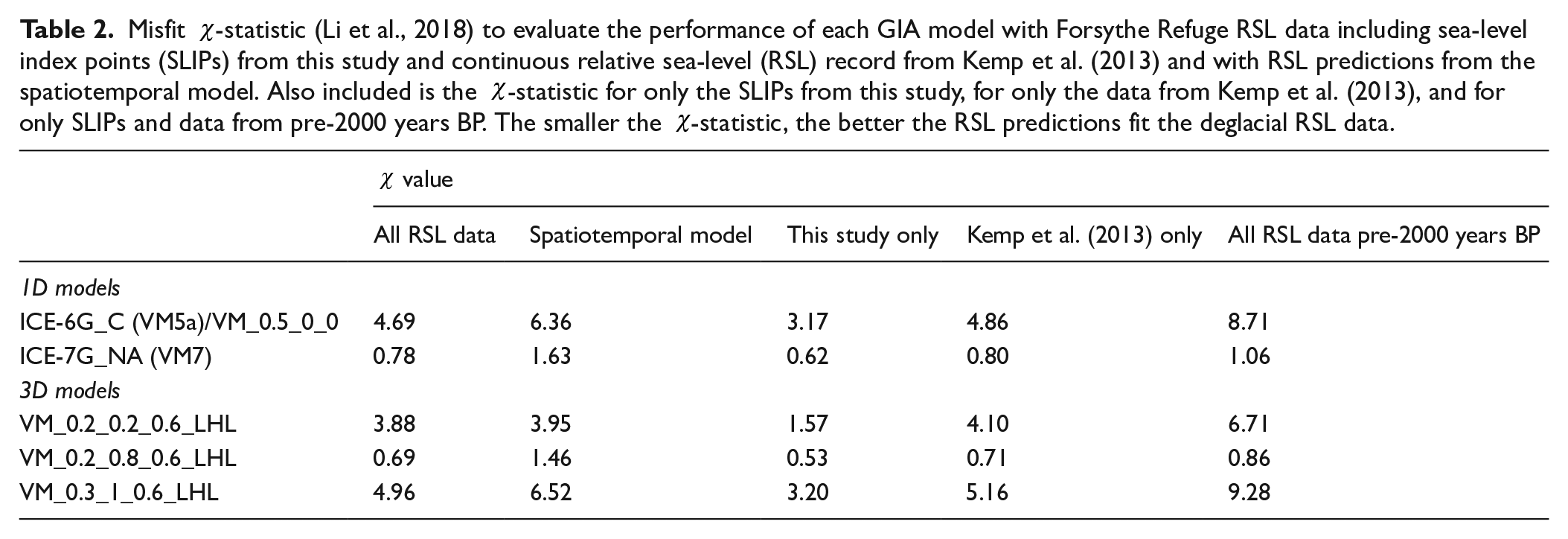
We compare the combined basal peat record at Forsythe Refuge and published RSL reconstruction (Kemp et al., 2013), as well as the RSL predictions at Forsythe Refuge from the spatiotemporal model, with five 1D and 3D GIA models (Figure 6). The 1D model ICE-6G_C (VM5a) performs poorly with the RSL data and has the misfit χ-statistic of 4.69 (6.36 with the spatiotemporal model results) (Table 2), as it overestimates the magnitude of RSL rise over the last 5000 years by ~7 m. The 1D model ICE-7G_NA (VM7) improves the fit and the χ-statistic decreases by 83.3% from 4.69 to 0.78 (74.4% from 6.36 to 1.63 with the spatiotemporal model results). The improvement of the fit is mainly due to viscosity modification in the lower mantle from VM5a to VM7, which focused exclusively on reconciling the model predictions with RSL data along the U.S. Atlantic coast (Roy and Peltier, 2015, 2017). The 3D GIA models show a wide range of predictions from overestimating by ~7 m (e.g. model VM_0.3_1_0.6_LHL) to slightly underestimating by ~1 m (e.g. model VM_0.2_0.2_0.6_LHL) the magnitude of RSL rise inferred from the data (Figure 6). Model VM_0.2_0.8_0.6_LHL provides the best fit with a χ-statistic of 0.69 (1.46 with the spatiotemporal model results) (Table 2). Model VM_0.2_0.8_0.6_LHL has a lower viscosity in the shallow lower mantle and higher viscosity in the deep lower mantle beneath southern New Jersey compared with VM5a (Figure 2 in Li et al. (2018) and is more consistent with viscosity variations in VM7 (Table 2 in Roy and Peltier (2017).

Table 2.

Misfit χ-statistic (Li et al., 2018) to evaluate the performance of each GIA model with Forsythe Refuge RSL data including sea-level index points (SLIPs) from this study and continuous relative sea-level (RSL) record from Kemp et al. (2013) and with RSL predictions from the spatiotemporal model. Also included is the χ-statistic for only the SLIPs from this study, for only the data from Kemp et al. (2013), and for only SLIPs and data from pre-2000 years BP. The smaller the χ-statistic, the better the RSL predictions fit the deglacial RSL data.

	χ value
	All RSL data	Spatiotemporal model	This study only	Kemp et al. (2013) only	All RSL data pre-2000 years BP
1D models
ICE-6G_C (VM5a)/VM_0.5_0_0	4.69	6.36	3.17	4.86	8.71
ICE-7G_NA (VM7)	0.78	1.63	0.62	0.80	1.06
3D models
VM_0.2_0.2_0.6_LHL	3.88	3.95	1.57	4.10	6.71
VM_0.2_0.8_0.6_LHL	0.69	1.46	0.53	0.71	0.86
VM_0.3_1_0.6_LHL	4.96	6.52	3.20	5.16	9.28

A single region does not have the statistical power to fully assess the performance of 3D models relative to 1D models, because of the additional parameters in 3D models. However, other analyses indicate that including 3D structure in the mantle and lateral thickness variation in the lithosphere has the capability to improve the fit with Holocene RSL at the scale of the Cascadia subduction zone to the whole North America continent (Clark et al., 2019; Kuchar et al., 2019; Li and Wu, 2019; Li et al., 2018; Love et al., 2016).

GIA prediction with uncertainties in southern New Jersey

On a broader regional scale, we compare the southern New Jersey sea-level database with the best-fitting GIA models that consider the prediction uncertainties from Li et al. (2020), which include an overall mean RSL prediction and 2σ uncertainties for each location. The sites in southern New Jersey (Forsythe Refuge, Sea Isle City, Brigantine, Whale Beach, Great Bay, Cape May Courthouse) are located within ~50 km of one another and therefore have similar mean predictions over the last 5000 years that vary by 0.1 m at 1000 years BP and up to 0.4 m at 5000 years BP. The 2σ uncertainties range for each southern New Jersey site is also similar, ranging at all sites from ~0.4 m at 1000 years BP to ~3 m at 5000 years BP. Figure 7 shows the average mean prediction for the southern New Jersey sites and the largest 2σ uncertainties, in addition to all of the southern New Jersey data and spatiotemporal model RSL predictions. The uncertainty band for each southern New Jersey site encompasses the RSL data, although the RSL data tend to sit above the mean GIA predictions from 3500 to 5000 years BP. The lack of fit may be due to not considering the uncertainty in the ice model and its interaction with the viscosity model.

Figure 7.

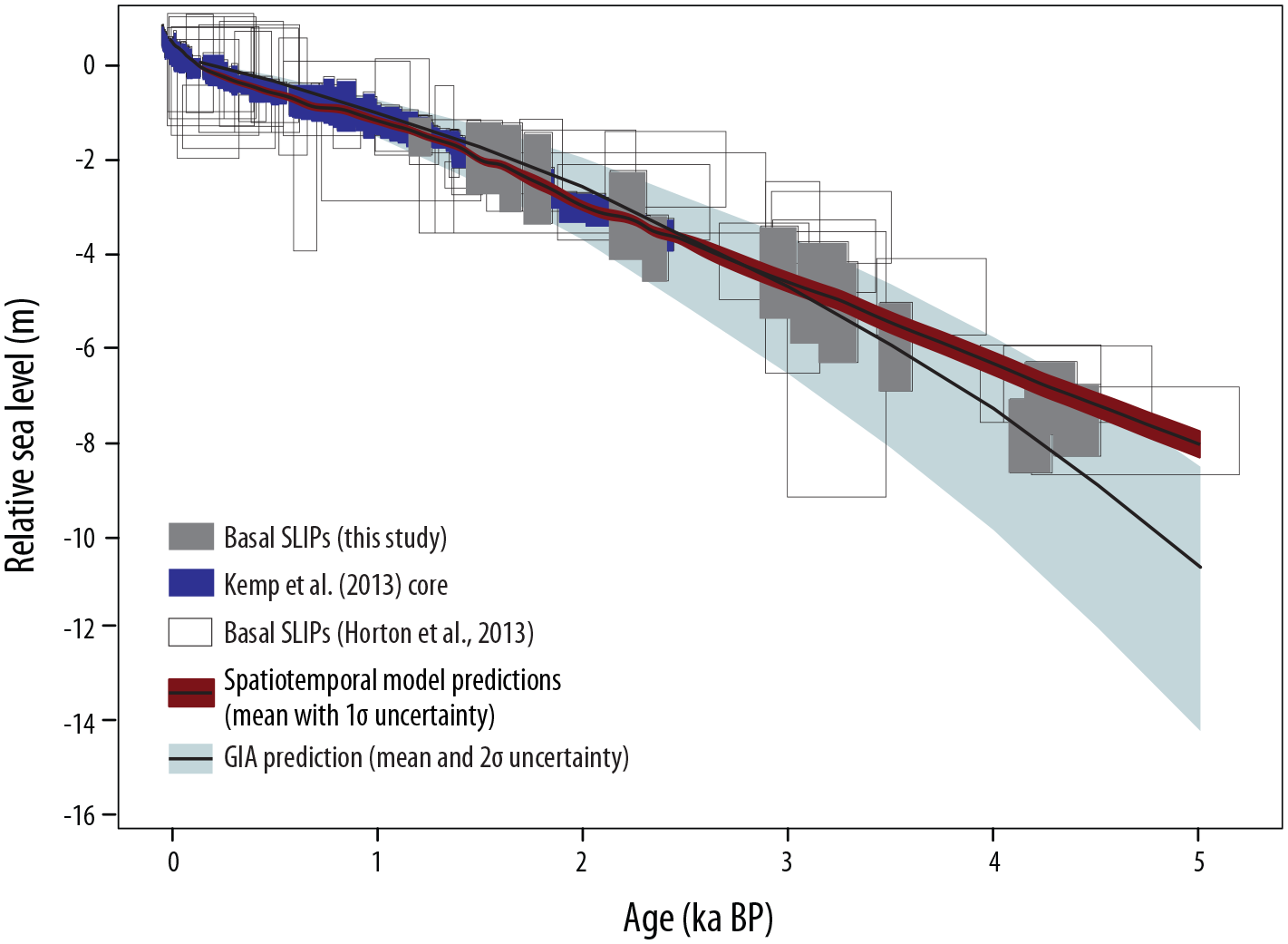
Southern New Jersey RSL dataset including: basal sea-level index points (SLIPs) from Forsythe Refuge (this study), continuous relative sea-level record from Kemp et al. (2013), and basal SLIPs from Horton et al. (2013). Spatiotemporal model predictions are shown with the mean and 1σ uncertainty. GIA model prediction from Li et al. (2020) includes an overall mean RSL prediction and 2σ uncertainties. SLIPs are plotted as boxes with 2σ vertical and calibrated age errors. The zero sea-level datum is at 150 years BP.

Interestingly, all five of the individual GIA models (Figure 6) and the best-fitting mean GIA predictions with uncertainties (Figure 7) exhibit a non-linear trend with decreasing rates of rise over the last 5000 years. For example, the rate of RSL of the mean GIA prediction decreases from 2.8 mm/year from 5000 to 2500 years BP to 1.5 mm/year from 2500 years BP to present. However, 94% of the variance in the RSL data in the southern New Jersey database (98% of the variance in the Forsythe Refuge RSL data in Figure 6) can be explained by a linear fit, suggesting the ice-equivalent component in the ice model may need to be refined (the ice-equivalent sea-level curves for ICE-6G_C and ICE-7G_NA are shown in Supplemental Figure 2). The Late-Holocene ice melt history has not been well resolved (Alley et al., 2010; Gehrels, 2010). The Greenland Ice Sheet (Long et al., 2012; Marcott et al., 2013; Mikkelsen et al., 2008; Sparrenbom et al., 2008) and small glaciers (Jansen et al., 2007) were growing in the Late-Holocene, so any Late-Holocene ice melt is likely due to Antarctica. Peltier (2002) argued that there was no ice melt after 4000 years BP (the ice melt from the Antarctica Ice Sheet (AIS) stops at 4000 years BP in ICE-6G_C (Argus et al., 2014; Peltier et al., 2015)), while Lambeck and Bard (2000) found a small (<0.5 m) component of ice-equivalent sea-level rise during the last 4000 years, and Lambeck (1988) argued that the AIS was contributing to sea-level rise as late as 2000 years BP. Furthermore, Bradley et al. (2016) concluded that the AIS contributed to an ice-equivalent sea-level rise of 1.7 m from 5000 years BP to ~1000 years BP. These model-based estimates are difficult to constrain as they rely on a small subset of global geological sea-level observations, and there are regional misfits between model outputs and observations (Gehrels, 2010). Lambeck et al. (2014) used ∼1000 observations from locations far from former ice margins and found a decline in the rate of sea-level rise from 6700 years BP with a rise of ⩽1 m from 4200 years BP to time of recent sea-level rise ~100–150 years ago. Love et al. (2016) used 35 North American ice complex model reconstructions (here we only use two ice models) and 363 different viscosity models to more precisely fit the GIA models to site-specific RSL data on the North American coastline, suggesting the importance of considering the uncertainty in GIA predictions that are associated with imperfect knowledge of ice and viscosity models. Further analyses involving uncertainty in Late-Holocene ice history and mantle viscosity, and the interaction between them, will continue to advance GIA model development and their fit to RSL data.

Conclusion

We reconstruct a new Mid- to Late-Holocene RSL record from a salt marsh in southern New Jersey using a multi-proxy approach of foraminifera and geochemistry coupled with ¹⁴C ages. We account for sediment compaction by using samples from basal peat units and a geotechnical model and for tidal range change by using a paleotidal model.

The 14 basal SLIPs range from 1211 ± 56 years BP to 4414 ± 112 years BP and show continuously rising RSL.

Using a spatiotemporal model with a database of southern New Jersey RSL data, we find that RSL rose by an approximate magnitude of 8.6 m at an average rate of 1.7 ± 0.1 mm/year (1σ) from 5000 years BP to present.

We compare our new RSL record and the southern New Jersey RSL database to an ensemble of 1D and site-specific 3D mantle viscosity models and best-fitting mean GIA predictions with uncertainties from Li et al. (2020). The model predictions tend to overestimate the magnitude of RSL rise over the last 5000 years compared to the RSL observations.

All of the 1D and 3D GIA models considered in this study cannot reproduce the linear trend revealed by the RSL data, which may imply the ice-equivalent sea-level signal in the ice models needs to be refined.

Supplemental Material

sj-docx-1-hol-10.1177_09596836221131696 – Supplemental material for A 5000-year record of relative sea-level change in New Jersey, USA

Supplemental material, sj-docx-1-hol-10.1177_09596836221131696 for A 5000-year record of relative sea-level change in New Jersey, USA by Jennifer S Walker, Tanghua Li, Timothy A Shaw, Niamh Cahill, Donald C Barber, Matthew J Brain, Robert E Kopp, Adam D Switzer and Benjamin P Horton in The Holocene

Footnotes

Acknowledgements

JSW thanks Isabel Hong, Kristen Joyse, and Andra Garner for their assistance in the field and thanks the Rutgers University Marine Field Station, Roland Hagan, and Ryan Larum for boat use in the field. We thank the Edwin B. Forsythe National Wildlife Refuge for providing access to study sites.

Funding

The author(s) disclosed receipt of the following financial support for the research, authorship, and/or publication of this article: JSW was funded by the David and Arleen McGlade Foundation and a Cushman Foundation for Foraminiferal Research Student Research Award. JSW and REK were also supported by US National Science Foundation awards OCE-1804999 and OCE-2002437. BPH, TL, and TS are supported by the Singapore Ministry of Education Academic Research Fund MOE2019-T3-1-004 and MOE-T2EP50120-0007, the National Research Foundation Singapore, and the Singapore Ministry of Education, under the Research Centres of Excellence initiative. NC is supported by the A4 project. A4 (Grant-Aid Agreement no. PBA/CC/18/01) is carried out with the support of the Marine Institute under the Marine Research Programme funded by the Irish Government. DCB receives support from the H.F. Alderfer Fund for Environmental Studies at Bryn Mawr College. The GIA modeling is conducted in part using the research computing facilities and/or advisory services offered by Information Technology Services, the University of Hong Kong. The authors acknowledge PALSEA (Palaeo-Constraints on Sea-Level Rise), a working group of the International Union for Quaternary Sciences (INQUA) and Past Global Changes (PAGES), which in turn received support from the Swiss Academy of Sciences and the Chinese Academy of Sciences. This work is a contribution to IGCP Project 725 “Forecasting Coastal Change.” This work is Earth Observatory of Singapore contribution 472.

ORCID iDs

Jennifer S Walker

Tanghua Li

Timothy A Shaw

Benjamin P Horton

Supplemental material

Supplemental material for this article is available online.

References

Allen

(2000) Morphodynamics of holocene salt marshes: A review sketch from the Atlantic and southern North Sea coasts of Europe. Quaternary Science Reviews 19: 1155–1231.

Alley

Andrews

Brigham-Grette

, et al. (2010) History of the Greenland ice sheet: Paleoclimatic insights. Quaternary Science Reviews 29: 1728–1756.

Argus

Peltier

Drummond

, et al. (2014) The Antarctica component of postglacial rebound model ICE-6G_C (VM5a) based on GPS positioning, exposure age dating of ice thicknesses, and relative sea level histories. Geophysical Journal International 198: 537–563.

Ashe

Cahill

Hay

, et al. (2019) Statistical modeling of rates and trends in Holocene relative sea level. Quaternary Science Reviews 204: 58–77.

Bloom

(1967) Pleistocene shorelines: A new test of isostasy. Geological Society of America Bullen 78: 1477–1494.

Bradley

Milne

Horton

, et al. (2016) Modelling sea level data from China and Malay-Thailand to estimate Holocene ice-volume equivalent sea level change. Quaternary Science Reviews 137: 54–68.

Brain

(2015) Compaction. In: Shennan

Long

Horton

(eds) Handbook of Sea-Level Research. Hoboken, NJ: John Wiley & Sons, Ltd, pp.452–469.

Brain

Kemp

Horton

, et al. (2015) Quantifying the contribution of sediment compaction to Late- Holocene salt-Marsh sea-level reconstructions, North Carolina, USA. Quaternary Research 83: 41–51.

Brain

Long

Petley

, et al. (2011) Compression behaviour of minerogenic low energy intertidal sediments. Sedimentary Geology 233: 28–41.

10.

Brain

Long

Woodroffe

, et al. (2012) Modelling the effects of sediment compaction on salt marsh reconstructions of recent sea-level rise. Earth and Planetary Science Letters 345–348: 180–193.

11.

Cahill

Kemp

Horton

, et al. (2016) A Bayesian hierarchical model for reconstructing relative sea level: From raw data to rates of change. Climate of the Past 12: 525–542.

12.

Chant

Curran

Able

, et al. (2000) Delivery of winter flounder (Pseudopleuronectes americanus) larvae to settlement habitats in coves near tidal inlets. Estuarine, Coastal and Shelf Science 51: 529–541.

13.

Clark

Mitrovica

Latychev

(2019) Glacial isostatic adjustment in central Cascadia: Insights from three-dimensional Earth modeling. Geology 47: 295–298.

14.

Clark

Farrell

Peltier

(1978) Global changes in postglacial sea level: A numerical calculation. Quaternary Research 9: 265–287.

15.

Daddario

(1961) A lagoon deposit profile near Atlantic City, New Jersey (No. 6). Bulletin of the New Jersey Academy of Science.

16.

Davis

Mitrovica

(1996) Glacial isostatic adjustment and the anomalous tide gauge record of eastern North America. Nature 379: 331–333.

17.

Edwards

(2006) Mid-to Late-Holocene relative sea-level change in southwest britain and the influence of sediment compaction. The Holocene 16: 575–587.

18.

Engelhart

Horton

(2012) Holocene sea level database for the Atlantic coast of the United States. Quaternary Science Reviews 54: 12–25.

19.

Engelhart

Horton

Douglas

, et al. (2009) Spatial variability of Late-Holocene and 20th century sea-level rise along the Atlantic coast of the United States. Geology 37: 1115–1118.

20.

Engelhart

Peltier

Horton

(2011) Holocene relative sea-level changes and glacial isostatic adjustment of the U.S. Atlantic coast. Geology 39: 751–754.

21.

Ferland

(1990) Holocene Depositional History of the Southern New Jersey Barrier and Backbarrier Regions (No. CERC-TR-90-2). Coastal Engineering Research Center Vicksburg MS.

22.

Field

Duane

(1976) Post-pleistocene history of the United States inner continental shelf: Significance to origin of barrier islands. Geological Society of America Bullen 87: 691–702.

23.

Gehrels

(2010) Sea-level changes since the last glacial maximum: An appraisal of the IPCC fourth assessment report. Journal of Quaternary Science 25: 26–38.

24.

Gehrels

(1994) Determining relative sea-level change from salt-marsh Foraminifera and plant zones on the coast of Maine, U.S.A. Journal of Coastal Research 10: 21.

25.

Gehrels

(1999) Middle and late Holocene sea-level changes in eastern Maine reconstructed from foraminiferal saltmarsh stratigraphy and AMS ¹⁴C dates on basal peat. Quaternary Research 52: 350–359.

26.

Gehrels

(2000) Using foraminiferal transfer functions to produce high-resolution sea-level records from salt-marsh deposits, Maine, USA. The Holocene 10: 367–376.

27.

Gehrels

Belknap

Pearce

, et al. (1995) Modeling the contribution of M2 tidal amplification to the holocene rise of mean high water in the Gulf of Maine and the Bay of Fundy. Marine Geology 124: 71–85.

28.

Gehrels

Dangendorf

Barlow

NLM

, et al. (2020) A preindustrial sea-level rise hotspot along the Atlantic coast of North America. Geophysical Research Letters 47: e2019GL085814.

29.

Gehrels

Milne

Kirby

, et al. (2004) Late Holocene sea-level changes and isostatic crustal movements in Atlantic Canada. Quaternary International, Coastal Environmental Change during Sea-Level Highstands, IGCP 437 Symposium, Barbados 120: 79–89.

30.

Gornitz

Seeber

(1990) Vertical crustal movements along the East Coast, North America, from historic and late holocene sea level data. Tectonophysics 178: 127–150.

31.

Griffiths

Hill

(2015) Tidal modeling. In: Shennan I, Long AJ and Horton BP (eds) Handbook of Sea-Level Research. Hoboken, NJ: John Wiley & Sons, Ltd. pp.438–451.

32.

Griffiths

Peltier

(2008) Megatides in the Arctic Ocean under glacial conditions. Geophysical Research Letters 35: L08605. DOI: 10.1029/2008gl033263

33.

Griffiths

Peltier

(2009) Modeling of Polar Ocean Tides at the last glacial maximum: Amplification, sensitivity, and climatological implications. Journal of Climate 22: 2905–2924.

34.

Hall

Hill

Horton

, et al. (2013) A high-resolution study of tides in the Delaware Bay: Past conditions and future scenarios. Geophysical Research Letters 40: 338–342.

35.

Hawkes

Kemp

Donnelly

, et al. (2016) Relative sea-level change in northeastern Florida (USA) during the last ∼8.0 ka. Quaternary Science Reviews 142: 90–101.

36.

Head

(2006) Manual of Soil Laboratory Testing—Volume 1: Soil Classification and Compaction Tests. Caithness, UK: Whittles Publishing, pp.131–382

37.

Head

Epps

(2011) Manual of Soil Laboratory Testing—Volume 2: Permeability, Shear Strength and Compressibility Tests. Caithness, UK: Whittles Publishing, pp.463–473.

38.

Hijma

Engelhart

Tornqvist

, et al. (2015) A protocol for a geological sea-level database. In: Shennan I, Long AJ and Horton BP (eds) Handbook of Sea-Level Research. Hoboken, NJ: John Wiley & Sons, Ltd, pp.536–556.

39.

Hill

Griffiths

Peltier

, et al. (2011) High-resolution numerical modeling of tides in the western Atlantic, Gulf of Mexico, and Caribbean Sea during the Holocene. Journal of Geophysical Research 116: C10014. DOI: 10.1029/2010jc006896

40.

Horton

Edwards

(2006) Quantifying holocene sea-level change using intertidal foraminifera: Lessons from the British Isles. Cushman Foundation for Foraminiferal Research Special Publication 29: 541–542.

41.

Horton

Edwards

Lloyd

(1999) A foraminiferal-based transfer function: Implications for sea-level studies. Journal of Foraminiferal Research 29: 117–129.

42.

Horton

Engelhart

Hill

, et al. (2013) Influence of tidal-range change and sediment compaction on Holocene relative sea-level change in New Jersey, USA. Journal of Quaternary Science 28: 403–411.

43.

Horton

Shennan

(2009) Compaction of holocene strata and the implications for relative sealevel change on the east coast of England. Geology 37: 1083–1086.

44.

Inman

Nordstrom

(1971) On the tectonic and morphologic classification of coasts. The Journal of Geology 79(1): 1–21.

45.

Jansen

Overpeck

Briffa

, et al. (2007) Palaeoclimate, in: Climate Change 2007: The Physical Science Basis. Contribution of Working Group I to the Fourth Assessment Report of the Intergovernmental Panel on Climate Change. Cambridge: Cambridge University Press, pp.433–497.

46.

Johnson

Moore

Lehmann

, et al. (2007) Middle to late Holocene fluctuations of C3 and C4 vegetation in a northern New England salt marsh, Sprague Marsh, Phippsburg Maine. Organic Geochemistry 38: 394–403.

47.

Kaufmann

Ivins

(2005) Lateral viscosity variations beneath Antarctica and their implications on regional rebound motions and seismotectonics. Journal of Geodynamics 39: 165–181.

48.

Kemp

Hill

Vane

, et al. (2017a) Relative sea-level trends in New York city during the past 1500 years. The Holocene 27: 1169–1186.

49.

Kemp

Kegel

Culver

, et al. (2017b) Extended late holocene relative sea-level histories for North Carolina, USA. Quaternary Science Reviews 160: 13–30.

50.

Kemp

Horton

Donnelly

, et al. (2011) Climate related sea-level variations over the past two millennia. Proceedings of the National Academy of Sciences of the United States of America 108: 11017–11022.

51.

Kemp

Horton

Vane

, et al. (2013) Sea-level change during the last 2500 years in New Jersey, USA. Quaternary Science Reviews 81: 90–104.

52.

Kemp

Vane

Horton

, et al. (2012) Application of stable carbon isotopes for reconstructing salt-marsh floral zones and relative sea level, New Jersey, USA. Journal of Quaternary Science 27: 404–414.

53.

Kemp

Wright

Edwards

, et al. (2018) Relative sea-level change in Newfoundland, Canada during the past ∼3000 years. Quaternary Science Reviews 201: 89–110.

54.

Khan

Horton

Engelhart

, et al. (2019) Inception of a global atlas of sea levels since the last glacial maximum. Quaternary Science Reviews 220: 359–371.

55.

Kominz

Miller

Browning

(1998) Long-term and short-term global Cenozoic sea-level estimates. Geology 26: 311–314.

56.

Kopp

Horton

Little

, et al. (2014) Probabilistic 21st and 22nd century sea-level projections at a global network of tide-gauge sites. Earth s Future 2: 383–406.

57.

Kopp

Kemp

Bittermann

, et al. (2016) Temperature-driven global sea-level variability in the common era. Proceedings of the National Academy of Science of the United States of America 113: E1434–E1441.

58.

Kuchar

Milne

Latychev

(2019) The importance of lateral earth structure for North American glacial isostatic adjustment. Earth and Planetary Science Letters 512: 236–245.

59.

Lambeck

(1988) The Earth’s variable rotation: Some geophysical causes. Symposium - International Astronomical Union 128: 1–20.

60.

Lambeck

Bard

(2000) Sea-level change along the French Mediterranean coast for the past 30 000 years. Earth and Planetary Science Letters 175: 203–222.

61.

Lambeck

Purcell

Zhao

(2017) The North American late Wisconsin ice sheet and mantle viscosity from glacial rebound analyses. Quaternary Science Reviews 158: 172–210.

62.

Lambeck

Rouby

Purcell

, et al. (2014) Sea level and global ice volumes from the last glacial maximum to the Holocene. Proceedings of the National Academy of Sciences 111: 15296–15303.

63.

(2019) Laterally heterogeneous lithosphere, asthenosphere and sub-lithospheric properties under Laurentia and Fennoscandia from glacial isostatic adjustment. Geophysical Journal International 216: 1633–1647.

64.

Steffen

, et al. (2018) In search of laterally heterogeneous viscosity models of glacial isostatic adjustment with the ICE-6G_C global ice history model. Geophysical Journal International 214: 1191–1205.

65.

Wang

, et al. (2020) Uncertainties of glacial isostatic adjustment model predictions in North America associated with 3D structure. Geophysical Research Letters 47: e2020GL087944.

66.

Long

Waller

Stupples

(2006) Driving mechanisms of coastal change: Peat compaction and the destruction of late holocene coastal wetlands. Marine Geology 225: 63–84.

67.

Long

Woodroffe

Milne

, et al. (2012) Relative sea-level change in Greenland during the last 700 yrs and ice sheet response to the little ice age. Earth and Planetary Science Letters 315-316: 76–85..

68.

Love

Milne

Tarasov

, et al. (2016) The contribution of glacial isostatic adjustment to projections of sea-level change along the Atlantic and Gulf coasts of North America. Earth s Future 4: 440–464.

69.

Luettich

Westerink

(1991) A solution for the vertical variation of stress, rather than velocity, in a three-dimensional circulation model. International Journal for Numerical Methods in Fluids 12: 911–928.

70.

Marcott

Shakun

Clark

, et al. (2013) A reconstruction of regional and global temperature for the past 11,300 years. Science 339: 1198–1201.

71.

Middelburg

Nieuwenhuize

Lubberts

, et al. (1997) Organic carbon isotope systematics of coastal marshes. Estuarine, Coastal and Shelf Science 45: 681–687.

72.

Mikkelsen

Kuijpers

Arneborg

(2008) The Norse in Greenland and late holocene sea-level change. Polar Record 44: 45–50.

73.

Miller

Kopp

Horton

, et al. (2013) A geological perspective on sea-level rise and its impacts along the U.S. mid-Atlantic coast. Earth s Future 1: 3–18.

74.

Miller

Sugarman

Browning

, et al. (2009) Sea-level rise in New Jersey over the past 5000 years: Implications to anthropogenic changes. Global and Planetary Change 66: 10–18.

75.

Milne

Mitrovica

(1998) The influence of time-dependent ocean-continent geometry on predictions of post-glacial sea level change in Australia and New Zealand. Geophysical Research Letters 25: 793–796.

76.

Mitrovica

Forte

(1997) Radial profile of mantle viscosity: Results from the joint inversion of convection and postglacial rebound observables. Journal of Geophysical Research Solid Earth 102: 2751–2769.

77.

Mofjeld

Venturato

González

, et al. (2004) The harmonic constant datum method: Options for overcoming datum discontinuities at mixed–diurnal tidal transitions. Journal of Atmospheric and Oceanic Technology 21: 95–104.

78.

Morris

Sundareshwar

Nietch

, et al. (2002) Responses of coastal wetlands to rising sea level. Ecology 83: 2869–2877.

79.

Peltier

(1994) Ice age Paleotopography. Science 265: 195–201.

80.

Peltier

(1998) The inverse problem for mantle viscosity. Inverse Problems 14: 441–478.

81.

Peltier

(2002) On eustatic sea level history: Last Glacial Maximum to Holocene.Quarternary Science Reviews , EPILOG 21: 377–396.

82.

Peltier

(2004) Global glacial isostasy and the surface of the Ice-Age Earth: The ICE-5G (VM2) model and GRACE. Annual Review of Earth and Planetary Sciences 32: 111–149.

83.

Peltier

Argus

Drummond

(2015) Space geodesy constrains ice age terminal deglaciation: The global ICE-6G_C (VM5a) model. Journal of Geophysical Research Solid Earth 120: 450–487.

84.

Peltier

Drummond

(2008) Rheological stratification of the lithosphere: A direct inference based upon the geodetically observed pattern of the glacial isostatic adjustment of the North American continent. Geophysical Research Letters 35: L16314. DOI: 10.1029/2008gl034586

85.

Psuty

(1986) Holocene sea level in New Jersey. Physical Geography 7: 156–167.

86.

Redfield

(1972) Development of a New England salt marsh. Ecological Monographs 42: 201–237.

87.

Rees

(ed.) (2014) Adaptive oedometer automation. The Geotechnica, 27–31.

88.

Reimer

Austin

WEN

Bard

, et al. (2020) The IntCal20 Northern Hemisphere radiocarbon age calibration curve (0–55 cal kBP). Radiocarbon 62: 725–757.

89.

Roy

Peltier

(2015) Glacial isostatic adjustment, relative sea level history and mantle viscosity: Reconciling relative sea level model predictions for the U.S. East coast with geological constraints. Geophysical Journal International 201: 1156–1181.

90.

Roy

Peltier

(2017) Space-geodetic and water level gauge constraints on continental uplift and tilting over North America: Regional convergence of the ICE-6G_C (VM5a/VM6) models. Geophysical Journal International 210: 1115–1142.

91.

Roy

Peltier

(2018) Relative sea level in the western Mediterranean basin: A regional test of the ICE-7G_NA (VM7) model and a constraint on late holocene Antarctic deglaciation. Quaternary Science Reviews 183: 76–87.

92.

Schmelz

Miller

Kopp

, et al. (2021) Influence of mantle dynamic topographical variations on US Mid-Atlantic continental margin estimates of sea-level change. Geophysical Research Letters 48: e2020GL090521.

93.

Scott

Medioli

(1978) Vertical zonations of marsh Foraminifera as accurate indicators of former sea-levels. Nature 272: 528–531.

94.

Shennan

(1986) Flandrian sea-level changes in the Fenland. II: Tendencies of sea-level movement, altitudinal changes, and local and regional factors. Journal of Quaternary Science 1: 155–179.

95.

Shennan

Coulthard

Flather

, et al. (2003) Integration of shelf evolution and river basin models to simulate holocene sediment dynamics of the Humber Estuary during periods of sea-level change and variations in catchment sediment supply. The Science of the Total Environment 314-316: 737–754.

96.

Shennan

Horton

(2002) Holocene land- and sea-level changes in great Britain. Journal of Quaternary Science 17: 511–526.

97.

Shennan

Lambeck

Flather

, et al. (2000) Modelling western North Sea palaeogeographies and tidal changes during the holocene. Geological Society London Special Publications 166: 299–319.

98.

Sparrenbom

Bennike

Björck

, et al. (2008) Holocene relative sea-level changes in the Qaqortoq area, southern Greenland. Boreas 35: 171–187.

99.

Steffen

Kaufmann

(2006) Three-dimensional finite-element modeling of the glacial isostatic adjustment in Fennoscandia. Earth and Planetary Science Letters 250: 358–375.

100.

Tarasov

Dyke

Neal

, et al. (2012) A data-calibrated distribution of deglacial chronologies for the North American ice complex from glaciological modeling. Earth and Planetary Science Letters 315-316: 30–40.

101.

Törnqvist

González

Newsom

, et al. (2004) Deciphering holocene sea-level history on the U.S. Gulf Coast: A high-resolution record from the Mississippi delta. Geological Society of America Bullen 116: 1026–1039.

102.

Törnqvist

Wallace

Storms

JEA

, et al. (2008) Mississippi delta subsidence primarily caused by compaction of holocene strata. Nature Geoscience 1: 173–176.

103.

Troels-Smith

(1955) Characterization of Unconsolidated Sediments. Geological Survey of Denmark, ser. IV, 3: 38–73.

104.

U.S. Fish & Wildlife Service (2020) Edwin B. Forsythe National Wildlife Refuge. Department of the Interior.

105.

Varekamp

Thomas

Plassche

(1992) Relative sea-level rise and climate change over the last 1500 years. Terra Nova 4: 293–304.

106.

Walker

Cahill

Khan

, et al. (2020) Incorporating temporal and spatial variability of salt-marsh Foraminifera into sea-level reconstructions. Marine Geology 429: 106293.

107.

Walker

Kopp

Little

, et al. (2022) Timing of emergence of modern rates of sea-level rise by 1863. Nature Communications 13: 966.

108.

Walker

Kopp

Shaw

, et al. (2021) Common era sea-level budgets along the U.S. Atlantic coast. Nature Communications 12: 1841.

109.

(2005) Effects of lateral variations in lithospheric thickness and mantle viscosity on glacially induced surface motion in Laurentia. Earth and Planetary Science Letters 235: 549–563.

110.

Peltier

(1984) Pleistocene deglaciation and the Earth’s rotation: A new analysis. Geophysical Journal International 76: 753–791.

111.

Yang

Myers

Wong

, et al. (2008) Vdatum for Chesapeake Bay, Delaware Bay, and Adjacent Coastal Water Areas: Tidal Datums and Sea Surface Topography.

112.

S-Y

Törnqvist

(2012) Quantifying holocene lithospheric subsidence rates underneath the Mississippi delta. Earth and Planetary Science Letters 331-332: 21–30.

Supplementary Material

Please find the following supplemental material available below.

For Open Access articles published under a Creative Commons License, all supplemental material carries the same license as the article it is associated with.

For non-Open Access articles published, all supplemental material carries a non-exclusive license, and permission requests for re-use of supplemental material or any part of supplemental material shall be sent directly to the copyright owner as specified in the copyright notice associated with the article.

0.00 MB

0.32 MB

A 5000-year record of relative sea-level change in New Jersey,USA

Abstract

Keywords

Introduction

Study area

Methods

Estimating paleomarsh elevation

Compaction

Tidal range change

Reconstructing relative sea level

GIA models

Relative sea-level reconstruction

Stratigraphy

Paleomarsh elevation

Compaction

Tidal range change

Sea-level index points

Discussion

New Jersey relative sea level

Comparison with individual GIA models

GIA prediction with uncertainties in southern New Jersey

Conclusion

Supplemental Material

sj-docx-1-hol-10.1177_09596836221131696 – Supplemental material for A 5000-year record of relative sea-level change in New Jersey, USA

Footnotes

Acknowledgements

Funding

ORCID iDs

Supplemental material

References

Supplementary Material