Sage Journals: Discover world-class research

Abstract

Stable carbon isotope analysis is increasingly used in archaeology as an indicator of crop water status and/or water management regime. While the technique shows promise, robust modern baseline studies are required to inform and validate archaeological interpretations. Here, we test stable carbon isotope values as a crop water status proxy in a monsoonal climatic context for the first time. Specifically, we test the relationship between grain stable carbon isotope values (δ¹³C_grain), water availability, irrigation and soil type in barley (Hordeum vulgare L. (Zohary and Hopf.)) in north-west India, with the aim of deriving a locally-appropriate model for isotopic interpretation. We test this relationship across a substantial rainfall gradient (200–1000 mm/year) and find a negative logarithmic relationship between climatic water availability and δ¹³C. However, there is significant noise in the relationship, and we report δ¹³C_grain variation of over 3‰ amongst samples drawn from similar climatic contexts. Soil type, irrigation type and irrigation frequency have no clear modifying effects. We conclude that: (1) barley stable carbon isotope values can act as an archaeological water status proxy in monsoonal areas, but will be most sensitive in areas receiving <450 mm rainfall per year; and (2) it is not possible to precisely infer water management regimes. On the basis of our results, we propose guidelines for archaeological barley stable carbon isotope interpretation in north-west India and analogous monsoonal climates.

Keywords

archaeology barley irrigation stable carbon isotope analysis water management water stress

Introduction

Stable carbon isotope analysis of crop remains is becoming increasingly popular as a means of reconstructing past plant water availability. In archaeology, it has gained particular interest as a crop water status proxy and/or for elucidating past water management regimes (Aguilera et al., 2011; Araus et al., 2014; Flohr et al., 2019; Riehl et al., 2008, 2014; Styring et al., 2016; Vaiglova et al., 2014; Wallace et al., 2015). Part of its popularity stems from its capacity to act as a direct physiological indicator of plant water status: meaning it does not rely on the availability of other forms of evidence (e.g. detectable irrigation infrastructure), and allows crop-specific inference of past water conditions. To date, the method has been applied in the Mediterranean, Near East, Central Europe and Britain, where it has been used to draw inferences on issues ranging from irrigation practices, crop yields, crop provenance and differential crop treatment, to climate change and climatic conditions at the emergence of agriculture (Aguilera et al., 2009, 2012; Araus et al., 2001, 2014; Bogaard et al., 2016; Ferrio et al., 2005; Fiorentino et al., 2012; Flohr et al., 2019; Lightfoot and Stevens, 2012; Masi et al., 2013; Riehl et al., 2008, 2014; Styring et al., 2016; Vaiglova et al., 2014; Wallace et al., 2015). This paper seeks to broaden the method’s applicability to monsoonal regions, by reporting a modern baseline study on barley (Hordeum vulgare) that has been grown in different soil and watering conditions in northwest India.

Principles of plant stable carbon isotopes as a water proxy

There is well-established theory underlying the use of stable carbon isotopes as a water status proxy (Cernusak et al., 2013; Farquhar et al., 1982, 1989; Tieszen, 1991). The technique is underpinned by the influence of water status on carbon isotope discrimination (Δ¹³C) during photosynthesis (Farquhar et al., 1982). It is particularly applicable in C₃ plants (the sole focus here), which encompass over 95% of the world’s plant species (Kohn, 2010) and include major food staples such as wheat, barley and rice. In C₃ plants, Δ¹³C is strongly influenced by plant water status because of the effect of water status on the degree of stomatal opening (Cernusak et al., 2013). In well-watered conditions, open stomata permit CO₂ to diffuse freely into the leaf, allowing the photosynthetic process to discriminate against the heavier ¹³C isotope (O’Leary, 1988). In drier conditions, closed stomata restrict the diffusion of CO₂, which reduces the isotopic discrimination. Plentiful water will thus tend to promote a high degree of carbon isotope discrimination (high Δ¹³C), while a water shortage will promote low carbon isotope discrimination (low Δ¹³C, Cernusak et al., 2013). This variation in Δ¹³C flows on to affect the stable carbon isotope value (δ¹³C) of the plant tissues that are produced from the photosynthetic sugars (Farquhar et al., 1989, see Supplemental Figure S1.1.1).

In areas where water limits plant growth – for example, arid and semi-arid zones – water status is generally the primary determinant of stomatal activity during photosynthesis, and therefore a dominant determinant of Δ¹³C (Cernusak et al., 2013). This association is reflected in a number of global and regional-scale meta-analyses, which have found clear positive relationships between moisture availability (generally as mean annual precipitation) and Δ¹³C (Diefendorf et al., 2010; Kohn, 2010). However, both Δ¹³C and the resulting plant tissue δ¹³C are also influenced by a myriad of other environmental and biological factors, including nutrient availability, light, altitude, temperature, water-logging and salinity, atmospheric CO₂ concentration, as well as genotypically- and environmentally-determined physiological characteristics (Cernusak et al., 2013; Farquhar et al., 1989; Hare et al., 2018; Tieszen, 1991; see summary in Supplemental Table S1.1.1).

One factor that is particularly important for archaeological studies is the impact of the δ¹³C_air value (of the atmospheric CO₂ source) on the final δ¹³C value of the plant tissue. In this paper, we focus specifically on δ¹³C_grain, although similar principles apply to charcoal and other types of plant sample. δ¹³C_air affects δ¹³C_grain because it impacts the stable carbon isotope composition of the plant sugars that are produced during photosynthesis, independent of the amount of carbon isotope discrimination. This relationship introduces complexity to archaeological interpretation because δ¹³C_air has varied substantially through time (Graven et al. 2017). Archaeological studies wishing to compare samples across time periods and/or with modern samples must therefore convert the measured δ¹³C values of the plant tissue samples to inferred Δ¹³C using (imperfect) estimates of past δ¹³C_air.

Overall, these factors reduce the precision with which: (a) variation in δ¹³C_grain can be attributed to variability in Δ¹³C, and (b) variation in (inferred) Δ¹³C can be attributed to variability in water conditions – which are themselves a complex balance of soil water holding capacity, various forms of water input, and water loss through runoff, evaporation and evapotranspiration. While not insurmountable, each of these components of uncertainty must be accounted for in archaeological stable carbon isotope applications.

Support for archaeological applications

In this context, archaeological applications of carbon isotopic analysis must be underpinned by robust modern baseline studies that define the relationship between climate, water management, plant water status, Δ¹³C and δ¹³C_grain in a way that supports a nuanced archaeological interpretation in given climatic settings. A number of such studies have now been undertaken in order to support stable carbon isotope interpretation in staple cereals (wheat and barley) and pulses (fava bean, lentil) in continental Europe, the European Mediterranean, north Africa and the Levant (Bogaard et al., 2016; Flohr et al., 2019; Styring et al., 2016; Wallace et al., 2013). These studies have resulted in several models (based on converted, i.e. inferred, Δ¹³C values) that have attempted either to quantify the relationship between Δ¹³C and precise water inputs (Araus et al., 1999; Ferrio and Voltas, 2005), or, more conservatively, establish broader relationships between Δ¹³C and ‘bands’ of plant water status and/or water management regime (Flohr et al., 2019; Wallace et al., 2013).

These interpretative frameworks have now been used to support a number of high impact archaeological applications (Araus et al., 2014; Styring et al., 2017), but a key gap in knowledge remains. To date, all interpretative frameworks have been based on results from baseline studies in Mediterranean climatic zones, where the dominant pattern is winter rainfall and hot dry summers. To support the broader application of the technique, research is needed to test the extent to which interpretative frameworks developed in these climatic contexts can be generalised to other ecological zones; providing locally-appropriate interpretative guidance as necessary (Flohr et al., 2019).

Here, we present the first baseline study of crop stable carbon isotope values in a monsoonal climatic zone (characterised by intense summer rainfall and, in general, low to no winter rainfall). As a case study, we examine barley (Hordeum vulgare L. (Zohary and Hopf.)) in monsoonal South Asia: specifically, the region of northwest India once occupied by the Indus Civilisation, which spread across the Indus River Basin and some of the surrounding regions (see Petrie, et al., 2017). Carbon isotope analysis has strong potential in this region, as there are steep rainfall gradients and water is scarce for some or all of the year in many areas. It is also a region where carbon isotope analysis is of strong archaeological interest: for example, there is intense debate about the extent and nature of irrigation utilised by Indus populations, and climate change-induced water scarcity has been invoked as a factor in the Indus Civilisation’s de-urbanisation (Miller, 2015; Petrie et al., 2017; Pokharia et al., 2013). In contrast to the Mediterranean contexts studied to date, much of the Indus River Basin has a monsoonal climate that brings rainfall predominantly in summer, rather than in the winter months, and often in rapid, intense bursts. This study thus seeks to: (a) provide a robust platform for carbon isotope analysis to be deployed specifically in this region’s monsoonal climatic context; and (b) serve as a broader test case to establish the degree to which frameworks developed under Mediterranean climatic regimes can be generalised to other ecological zones. We focus on H. vulgare because it is a common cereal in the archaeobotanical record across a climatically diverse portion of Eurasia (Bates, 2016; Liu et al., 2017), making it a crop for which interpretative frameworks have broad applicability.

This study assesses the relationship between stable carbon isotope values, climatic water availability, water management, soil conditions and sub-species (six-row vs two-row barley) in H. vulgare across a climatic gradient in northwest India. We take a field collection rather than a controlled experimental approach in order to best reflect the uncertainty inherent in archaeological contexts, and explicitly model irrigation, soil texture and salinity effects. This is the first time such a wide range of influences on Δ¹³C has been included in a modern baseline study. Due to the uncertainty introduced by δ¹³C_grain to Δ¹³C conversions, we use δ¹³C_grain in our statistical modelling. We then use our data to derive a set of principles to guide archaeological Δ¹³C interpretation in NW India and climatically analogous zones.

We specifically ask:

(i) Is δ¹³C_grain related to climatic water availability in H. vulgare in northwest India?

(ii) Does this relationship vary with irrigation, soil texture, water logging, salinity and/or sub-species (six-row vs two-row barley)?

Material and methods

Sample collection

Samples of H. vulgare were collected in northwest India over a climatic gradient of 200–1000 mm rainfall per year (Figure 1). Our sampling transect extended over approximately 400 km, running approximately south-west to north-east. Our first sampling campaign was carried out from 14 to 20 March 2014 and over 80% of samples were collected in this season. We undertook a follow-up trip to boost sampling coverage in March 2015. March equates to harvest time for H. vulgare in this region.

Figure 1.

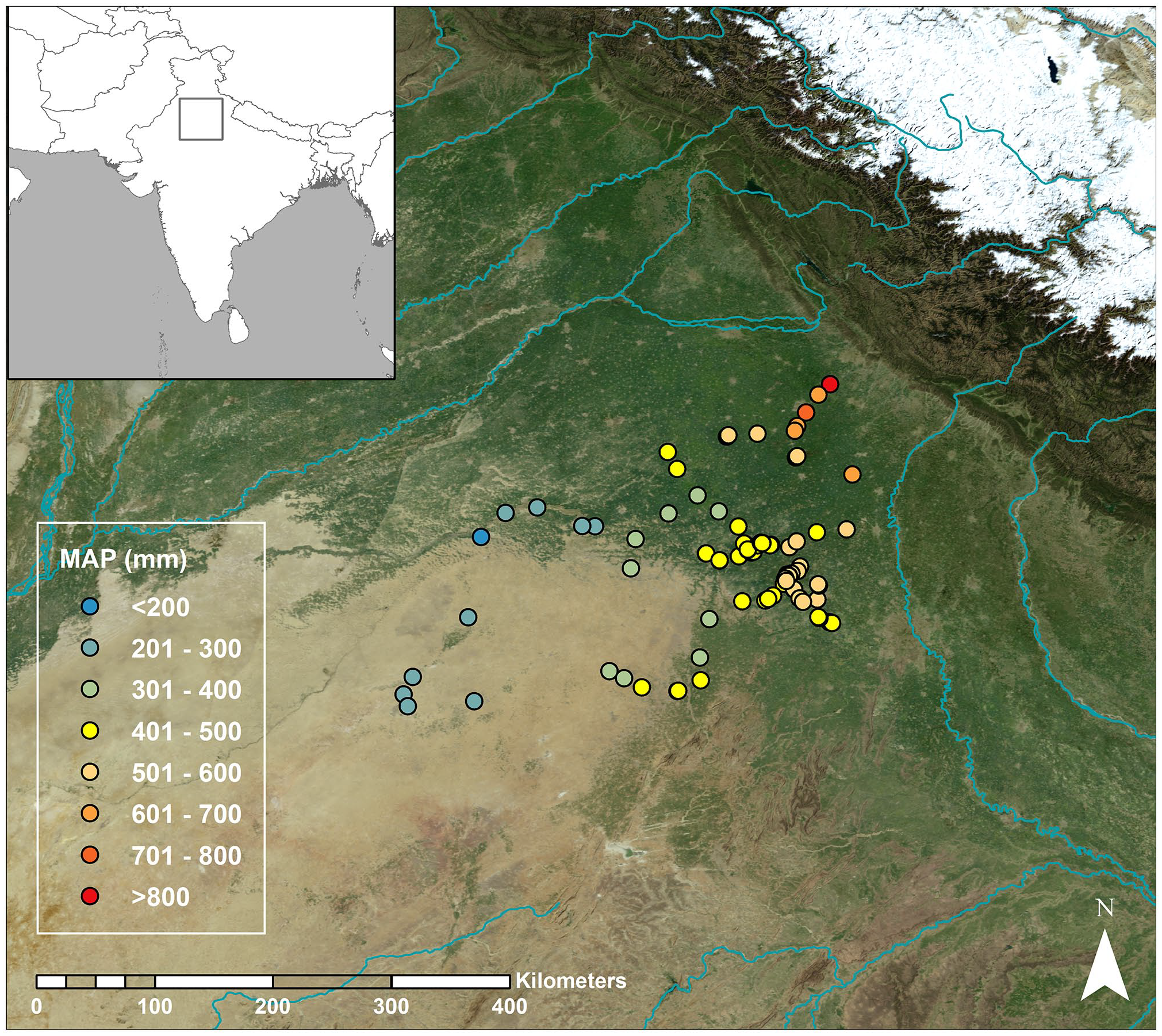
Map of north-west Indian Hordeum vulgare collection sites. Coding shows mean annual precipitation (MAP).

Sampling was based around ‘nodes,’ which were either villages/towns or significant archaeological sites. At each node, samples were collected from multiple sampling sites (that is, fields) in order to: (i) ensure sampling captured a broad representation of the local isotopic range, and (ii) enable sampling of plants grown under the same climatic conditions but under different irrigation regimes, on different soil types, or where the plants were of different phenotypes, in order to test for interactive effects.

At each sampling site, we collected samples of H. vulgare ears from: (a) standing plants within two-three weeks of harvesting, or (b) just-harvested material that was still in the field. Whole ears were taken from 15 to 20 individual plants, distributed across as much of each field as possible, but avoiding the outer ~50 cm to circumvent potential edge effects (Flohr et al., 2016).

At eight sampling sites it was evident that there was considerable intra-site heterogeneity in water availability and/or another variable of interest (soil texture, salinity or waterlogging severity). In these cases, we took separate samples from each clearly distinct ‘patch’ and recorded between-patch differences in plant, soil and water conditions. Similarly, where we could identify multiple phenotypes, we collected and analysed each phenotype separately to evaluate within-field, between-phenotype variation. In total we collected 124 samples from 87 sites across 37 nodes. Full details of all sampling locations are available in Supplemental Appendix S2.

At each sampling site, farmers were interviewed about their water management practices, plant varieties and recent weather conditions. We also photographed each sampling site and recorded details including GPS location, soil type, irrigation regime and topography. Collected samples were stored in sealed plastic bags at −20°C.

Laboratory protocol and mass spectrometry

For each sample, we stripped and pooled the grains from all ears and then randomly selected approximately 30 grains for carbon isotopic analysis. Initially, the grains were de-husked using a Qiagen tissue-lyser to maximise comparability with archaeological samples from the Indus region, the majority of which are unhulled. The grains were then ground to a fine powder using a Fisher Scientific ball-mill in order to homogenise the grains to give an average isotopic value for the growing conditions. The powder was freeze dried.

The ground samples were weighed into tin capsules for carbon isotope analysis in triplicate. Carbon isotope analysis was carried out at the Godwin Laboratory, Cambridge, using an automated Costech elemental analyser coupled in continuous flow mode to a ThermoFinnigan MAT253 mass spectrometer. Isotope values were measured as delta values (e.g. δ¹³C) relative to the international reference scale VPDB. Measurement uncertainty for δ¹³C was monitored using the international standard of caffeine (δ¹³C = −27.50; IAEA-600, IAEA, Vienna, Austria), and the in-house standards of nylon (δ¹³C: −26.6‰; size standard, nylon 6, Sigma-Aldrich, Gillingham, UK), alanine (δ¹³C: −26.9‰; L-alanine, Honeywell Fluka, Bucharest, Romania), protein 2 (δ¹³C: −27.0‰; Protein standard OAS, Elemental Microanalysis, Okehampton, UK), and again caffeine (δ¹³C: −35.9‰; Elemental Microanalysis). Standard materials comprised >10% of each isotopic run (Szpak et al., 2017). Using the procedures and spreadsheet provided by Szpak et al. (2017), precision (u(Rw)) was determined to be ±0.40‰ for δ¹³C on the basis of repeated measurements of both the international and in-house calibration standards, and on the measurements of sample replicates.

Environmental variable estimation

In order to model the relationship between δ¹³C_grain, water availability and potential confounding factors, we collated the following environmental variables for each sample: climatic water availability (i.e., the climatically driven component of water availability), irrigation inputs (i.e. the anthropogenic component of water availability), soil texture, salinity, water-logging status and two-row versus six-row sub-species. We were not able to obtain quantitative estimates of irrigation inputs from farmers, we thus categorised samples by irrigation type (flood/sprinkler/rainfed) and irrigation frequency (the number of times irrigated over the course of the growing season) on the basis of farmer information. Soil texture, salinity and water-logging were graded on the basis of field observation.

In order to estimate the climatically-driven component of water availability for each sampling site (i.e. water availability un-mediated by irrigation and soil type), we used global climate and hydrology grids. As there is no consensus over which measure of climatic water availability is most appropriate in baseline studies such as this, we compiled precipitation and temperature estimates from WorldClim; the aridity index (AI) from the CGIAR-CSI Global-Aridity and Global-PET Database; and soil water content (SWC) from the CGIAR-CSI Global Soil-Water Balance Database (Trabucco and Zomer, 2010; Trabucco et al., 2008; WorldClim, 2012). All are widely-recognised global models with a spatial resolution of ~1 km² (see Trabucco and Zomer, 2010; Trabucco et al., 2008; WorldClim, 2012 for details). Monthly estimates for each sampling site were extracted from the source databases using ArcGIS version 10.3; values are based on multi-year trends (from 1950 to 2000) and thus represent average climatic/hydrological conditions. While sampling-year specific data would have been advantageous, no 2014/2015 data were available with sufficient spatial resolution.

We then conducted a preliminary analysis to select the most appropriate proxy for use in our main analysis. On the basis of this preliminary analysis, we modelled soil water content (SWC) calculated over the growth cycle of October to March as our climatic water availability proxy. For full details and justification see Supplemental Section S1.3.

Statistical analysis

We used multiple linear regression models to test the relationship between δ¹³C_grain, climatic water availability (as measured by SWC), irrigation and soil type. SWC was centred in all models and log-transformed to achieve linearity. Irrigation and soil texture have the potential to interact but had to be assessed separately because not all soil types were present in all irrigation categories and vice versa. We therefore analysed irrigation and soil texture using separate regression models but performed supplementary analyses on restricted subsets of samples to test for confounding effects. We also performed a sensitivity analysis with data from 2014 only to check whether including data from 2 years introduced additional variability or otherwise impacted our results.

The impacts of salinity, waterlogging and two-row versus six-row sub-species on the δ¹³C_grain/water availability relationship were assessed via intra-site or reduced data-set analyses because the number and distribution of samples did not allow for integration into the main regressions. All analyses were performed in R (version 3.4.4) using the base, user-friendly science and car statistics packages (Fox and Weisberg, 2011; Peters, 2015; R Development Core Team, 2018).

Conversion to Δ¹³C

When we converted δ¹³C_grain results into Δ¹³C to facilitate comparison with archaeological and other modern baseline studies, we used the following equation (Farquhar et al., 1982):

\frac{δ^{13} C_{a i r} - δ^{13} C_{p l a n t}}{1 + δ^{13} C_{p l a n t} / 1000}

A key consideration in Δ¹³C conversion is the choice of value for δ¹³C_air. In addition to long term (centennial to millennial scale) variation, δ¹³C_air varies both seasonally and geographically. However, no seasonally resolved δ¹³C_air measurements from our study region or elsewhere in South Asia were obtainable. In our conversion we therefore used the 2014 and 2015 estimates of global mean δ¹³C_air from a compilation based on flask measurements, which are −8.42‰ and −8.44‰ respectively (Graven et al., 2017). These values differ substantively from the −8.00‰ that has been applied in a number of previous baseline studies (Flohr et al., 2011; Wallace et al., 2013); a difference that partially reflects the rapid change in δ¹³C values over the past two decades. While the best estimate available, the seasonal and geographical variation in δ¹³C_air means that the δ¹³C value of the atmospheric carbon that was assimilated into our sampled grains may differ from the global annual average estimate of Graven et al. (2017). Based on the degree of seasonal and spatial variation in δ¹³C across sites from the NOAA Earth System Research Laboratories network, we apply an estimated uncertainty of ±0.4‰ on our chosen value for δ¹³C_air into our Δ¹³C conversion to account for potential error. For full justification of our choice of δ¹³C_air and the ±0.4‰ uncertainty, see Supplemental Section S1.4.

Results

The relationship between δ¹³C_grain and climatic water availability

Our field collections yielded H. vulgare samples from 124 ‘patches’ at 87 sites across a gradient of 194–1042 mm mean annual precipitation (MAP) (Figure 1). The range of δ¹³C across all samples was −21.2‰ to −28.6‰ (Table 1, full raw data in Supplemental Appendix S3).

Table 1.

Summary statistics for H. vulgare δ¹³C and converted Δ¹³C (‰) by irrigation type.

	Irrigation type	n	Mean	SE	SD	Min	Max	Range
δ¹³C	Rainfed	4	−25.2	1.3	2.7	−27.5	−21.3	6.2
	Sprinkler	19	−24.8	0.3	1.3	−26.8	−22.0	4.8
	Flood	101	−26.0	0.1	1.4	−28.6	−21.2	7.4
	Overall	124	−25.8	0.1	1.5	−28.6	−21.2	7.4
Δ¹³C	Rainfed	4	17.2	1.4	2.8	13.2	19.6	6.4
	Sprinkler	19	16.8	0.3	1.4	13.9	18.9	5.0
	Flood	101	18.0	0.1	1.5	13.0	20.7	7.7
	Overall	124	17.8	0.1	1.5	13.0	20.7	7.7

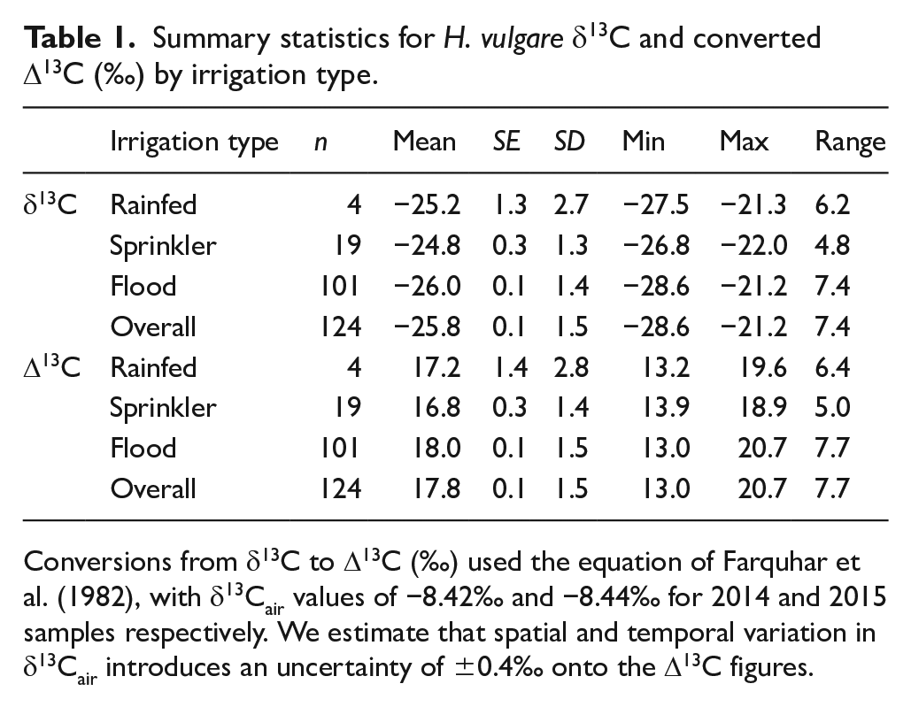
Conversions from δ¹³C to Δ¹³C (‰) used the equation of Farquhar et al. (1982), with δ¹³C_air values of −8.42‰ and −8.44‰ for 2014 and 2015 samples respectively. We estimate that spatial and temporal variation in δ¹³C_air introduces an uncertainty of ±0.4‰ onto the Δ¹³C figures.

Our first aim was to test the relationship between δ¹³C_grain and climatic water availability (as measured by soil water content, SWC). We found a negative logarithmic association between soil water content and δ¹³C_grain, though with wide scatter in the relationship (δ¹³C_grain = ln(SWC), adjusted R² = 0.18, beta = −1.77 ± 0.33SE, Figure 2, Table 2, Model H1A).

Figure 2.

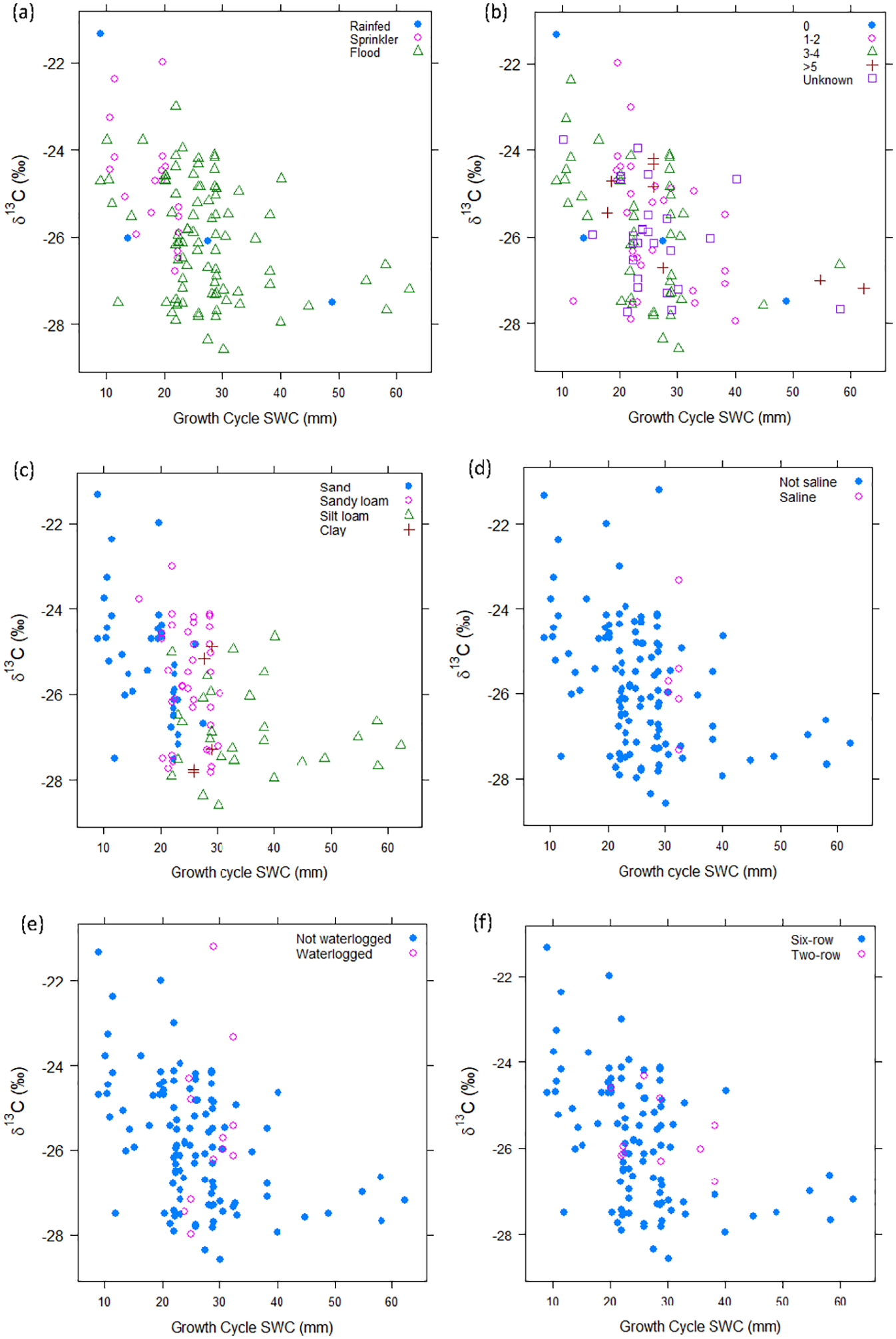
Modern NW Indian H. vulgare δ¹³C (‰), plotted against October to March Soil Water Content (SWC, mm) and distinguished by: (a) irrigation type, (b) irrigation frequency (the number of times irrigated over the growing season), (c) soil texture, (d) salinity status, (e) waterlogging status, and (f) six row versus two-row subspecies. Note that although the SWC data were log transformed for analysis, here we present the untransformed data in order to show the shape of the relationship and inflection point.

Table 2.

Results of regression models used to evaluate the effects of climatic water availability, irrigation and soil type on modern NW Indian H. vulgare δ¹³C.

Model	Excluded samples	Formula	n	Adjusted R²	p-Value – model	Predictor term	Baseline category	Beta	Beta SE	Std. beta	p-Value – predictor
1A	None	δ¹³C = ln(SWC)	124	0.18	>0.0001	ln(SWC)	n/a	−1.77	0.33	−0.43	<0.0001
1B	Saline	δ¹³C = ln(SWC)	111	0.24	>0.0001	ln(SWC)	n/a	−1.90	0.32	−0.49	<0.0001
1B	Waterlogged	δ¹³C = ln(SWC)	111	0.24	>0.0001	ln(SWC)	n/a	−1.90	0.32	−0.49	<0.0001
2	Saline	δ¹³C = ln(SWC) × irrigation type	111	0.26	>0.0001	ln(SWC)	n/a	−1.30	0.39	−0.34	0.001
	Waterlogged	δ¹³C = ln(SWC) × irrigation type				Sprinkler	Flood	0.41	0.46	0.15	0.37
						Rainfed	Flood	0.22	0.65	0.06	0.73
						ln(SWC) × Sprinkler	Flood	−1.06	1.13	−0.37	0.35
						ln(SWC) × Rainfed	Flood	−1.76	1.03	−0.46	0.09
3	Saline	δ¹³C = ln(SWC) x	108	0.19	>0.0001	ln(SWC)	n/a	−1.52	0.95	−0.39	0.11
	Waterlogged	Irrigation frequency				Irrig 3–4x	Irrig 1-2x	0.28	0.32	−0.12	0.40
	Rainfed					Irrig ⩾5x	Irrig 1-2x	0.56	0.58	0.14	0.33
						ln(SWC) × Irrig 3–4x	Irrig 1-2x	−0.49	1.07	−0.21	0.65
						ln(SWC) × Irrig ⩾5x	Irrig 1-2x	−0.47	1.45	−0.12	0.75
4	Saline	δ¹³C = ln(SWC) x	111	0.28	<0.001	ln(SWC)	n/a	−2.19	0.61	−0.57	<0.0001
	Waterlogged	Soil texture				Sandy loam	Sandy	0.32	0.35	0.20	0.35
						Silt loam	Sandy	−0.76	0.46	−0.20	0.09
						Clay	Sandy	−2.84	1.59	−1.76	0.07
						ln(SWC) × Sandy loam	Sandy	0.40	1.50	0.11	0.79
						ln(SWC) × Silt loam	Sandy	1.82	0.98	1.13	0.06
						ln(SWC) × Clay	Sandy	17.91	10.55	4.70	0.09

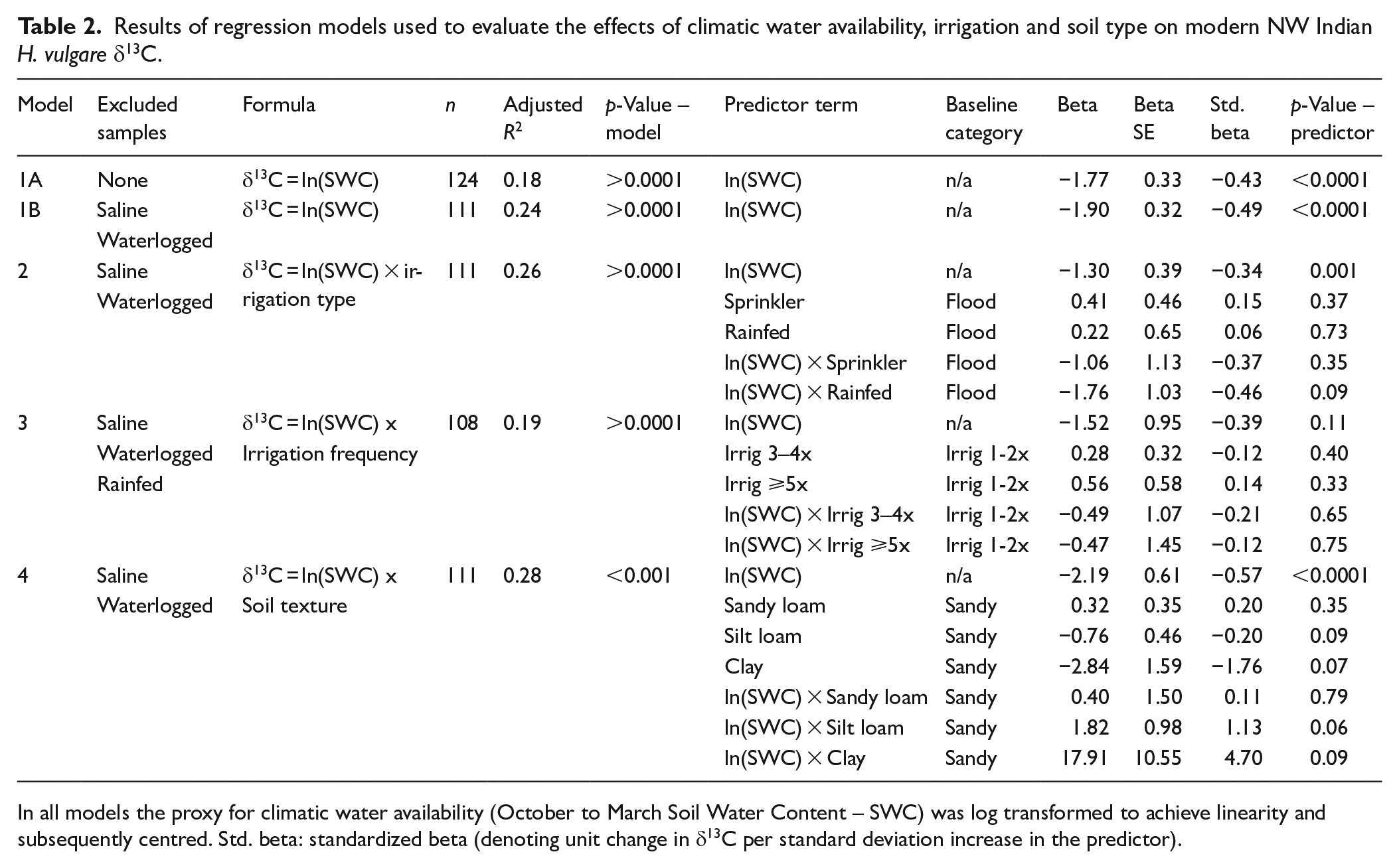
In all models the proxy for climatic water availability (October to March Soil Water Content – SWC) was log transformed to achieve linearity and subsequently centred. Std. beta: standardized beta (denoting unit change in δ¹³C per standard deviation increase in the predictor).

Thirteen of the 124 samples were from saline and/or waterlogged patches. As noted, salinity and waterlogging can affect Δ¹³C, and thus δ¹³C _grain, independent of water availability (Cernusak et al., 2013). After removing these 13 samples, there was a tighter relationship between δ¹³C_grain values and SWC (adjusted R² = 0.24, full details in Table 2, Model H1B). On this basis, samples affected by salinity and waterlogging were removed from all further regression analyses. Their impact was investigated separately via targeted comparisons (see below).

Our sensitivity analysis with 2014 data only returned virtually identical results to the all-samples analysis; we therefore included both 2014 and 2015 data in all further analyses.

Effects of irrigation, soil texture, waterlogging, salinity and sub-species

Our second aim was to test the effect of irrigation, soil texture, waterlogging, salinity and sub-species (six-row vs two-row) on the relationship between climatic water availability and δ¹³C_grain. We assessed irrigation effects in terms of: (a) irrigation type, and (b) irrigation frequency, as it was not possible to obtain quantitative irrigation input estimations.

Irrigation type

We found no marked or consistent offset between rainfed, sprinkler and flood irrigated samples within any climatic water availability band. The data show a negative logarithmic relationship between δ¹³C_grain and SWC regardless of irrigation type (Figure 2a). Adding irrigation type to the regression model as an interaction term did not improve the model fit (adjusted R² 0.26 compared to 0.24 for the baseline model, ANOVA comparing δ¹³C_grain = ln(SWC*IrrigType) to δ¹³C_grain = ln(SWC): F = 1.71, p = 0.15). SWC remained the dominant predictor of δ¹³C_grain in the irrigation type model (beta = −1.30 ± 0.39, standardised beta = −0.34). Sprinkler and rainfed irrigation had a minimal independent effect on δ¹³C_grain (large standard errors and small standardized betas, for full details see Table 2, Model 2).

A supplementary analysis controlling for the effect of soil type (by using sandy-soil samples only) returned very similar results to the whole-of-dataset analysis, indicating that these results are not an artefact of soil-type effects. Full details of this analysis are in Supplemental Table S1.5.1 and Figure S1.5.5).

Irrigation frequency

As shown in Figure 2b, there was no consistent offset between more and less frequent irrigation within any given climatic water availability band. Adding irrigation frequency to the regression model as an interaction term did not improve the model fit (adjusted R² was 0.19 for δ¹³C_grain = ln(SWC)*irrigfreq compared to 0.24 for the baseline model, ANOVA comparing δ¹³C_grain = ln(SWC*Irrigfreq to δ¹³C_grain = ln(SWC): F = 0.72, p = 0.58). As for irrigation type, SWC remained the dominant predictor in the irrigation frequency model (beta = −1.52 ± 0.95, standardized beta = −0.39). The coefficients for all irrigation frequency groups and their interactions had large standard errors and p-values >0.3 (full details in Table 2, Model 3). A supplementary analysis controlling for the effect of soil type returned very similar results to the whole-of-dataset analysis, for full details see Supplemental Table S1.5.1 and Figure S1.5.5.

Soil properties

Soil types were distributed unevenly across the climatic water availability gradient (Supplemental Figure S1.2.1), but where they overlap there was no consistent offset between the soil texture categories (Figure 2c). The power of the regression model including soil type was limited by the uneven soil type distribution, however the results confirm that regardless of soil type, ln(SWC) remains a strong predictor of δ¹³C_grain (beta = −2.19 ± 0.98, standardised beta = −0.57, for full results see Table 2, Model 4). There are possible but inconclusive indications of subtle soil texture effects: silt loam and clay both had negative coefficients – the direction that is consistent with greater water availability compared to the baseline of sand – with p-values between 0.05 and 0.10. The interactions between silt loam and clay with SWC also had p-values between 0.05 and 0.10 (details in Table 2, Model 4). Overall, adding soil type to the regression model marginally improved model fit to an adjusted R² of 0.28, compared with 0.24 for the baseline model (ANOVA comparing this regression with the baseline model, F = 1.8, p = 0.10).

Results from a reduced data-set analysis controlling for irrigation type mirror those of this overall analysis, indicating that the results are not due to confounding. Full results of the reduced data-set analysis are in Supplemental Table S1.5.1 and Figure S1.5.6.

Waterlogging and salinity

Waterlogging and/or salinity were visibly evident at 13 sites (11 of which were waterlogged; five of which were saline). As illustrated in Figure 2d and e, neither the waterlogged nor the saline sites are consistently offset compared to others in the same climatic band. This distribution indicates that the impacts of salinity and waterlogging are not clearly discernible from other sources of variability on an inter-site basis.

The impact of these variables on δ¹³C_grain was more apparent on an intra-site basis (illustrated in Supplemental Figure S1.5.3). In the fields subject to salinity, we found intra-site ranges between more and less saline patches of 0.3‰–2.2‰. The largest range was in the field with the sample with the least negative δ¹³C_grain value (suggesting greatest salinity stress). With respect to the fields with more and less waterlogged patches, one displays an extreme range of >6‰, with a very high δ¹³C_grain (−21.1‰) for the severely waterlogged area. In all cases the direction of difference in δ¹³C_grain accords with theoretical expectations that the more stressed patch should display the highest (least negative) δ¹³C_grain.

Six-row versus two-row sub-species

There is no systematic disparity between two-row and six-row barley samples across sites once climatic water availability is taken into account (although no two-row samples have values >−27.0‰, see Figure 2f).

At seven sampling sites we had the opportunity to compare δ¹³C_grain directly across co-cultivated varieties. In some cases, these included both two-row and six-row varieties, in others all co-occurring varieties were six-row but were clearly phenotypically distinct. The intra-site, inter-variety range was <1.6‰ in all but one field in which there was also a difference in irrigation regime (Supplemental Figure S1.4.4). Where both two- and six- row barley co-occurred, there was no systematic trend as to which form had the higher δ¹³C_grain.

Conversion to Δ¹³C

When converted into Δ¹³C for comparison with archaeological and other modern baseline studies, the Δ¹³C values of our samples range between 13.0‰ and 20.7‰ (Table 1, see also Figure 3). The range in converted values is slightly larger (7.7‰) than the δ¹³C_grain range, due to the slight difference in δ¹³C_air between our two sampling years, 2014 and 2015. As noted above, we applied an uncertainty of ±0.4‰ onto our converted values due to uncertainty in δ¹³C_air. This is shown as error bars in Figure 3.

Figure 3.

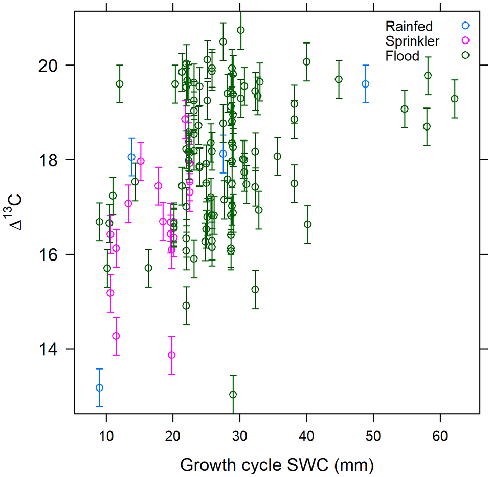
Converted modern NW Indian H. vulgare Δ¹³C (‰), plotted against October to March Soil Water Content (SWC, mm) and irrigation type. Δ¹³C conversions used the 2014 and 2015 global average estimates of δ¹³C_air derived from Graven et al. (2017). We estimate an uncertainty of ±0.4‰ on these δ¹³C_air estimates due to spatial and seasonal variation in δ¹³C_air, shown as error bars. Climatic water availability is measured by the growing cycle (October to March) Soil Water Content (SWC, mm).

Discussion

What is the relationship between δ¹³C_grain and climatic water availability?

Our results show a clear negative logarithmic relationship between H. vulgare δ¹³C_grain and soil water content (SWC), our chosen proxy for climatic water availability, across monsoonal northwest India. The logarithmic shape of the relationship indicates that climatic water availability more strongly influences δ¹³C_grain in the drier parts of our study region and less so in moister areas. This pattern reflects the tendency for water to limit stomatal opening (and thus carbon isotope discrimination) more strongly in arid zones. At the upper end of the water availability spectrum, water becomes less limiting, and we see this reflected via a marked flattening of the δ¹³C_grain water availability relationship in moister areas. This trend is in line with both theoretical expectations, other H. vulgare baseline studies, and global-scale, multi-taxon studies, where Δ¹³C appears nearly constant in humid climates (e.g. Diefendorf et al., 2010; Kohn, 2010). In this study, we found the most pronounced flattening of the carbon isotopic/climatic water availability relationship at values around 30–40 mm in October to March SWC (see Figure 2), which equates to approximately 550–600 mm mean annual precipitation.

Importantly, however, the relationship between soil water content and δ¹³C_grain was characterised by significant δ¹³C_grain variation amongst samples from sites experiencing similar climatic conditions. Indeed, across the whole study, the proportion of δ¹³C_grain variance explained by climatic water availability was low at just R² = 0.24 even after samples from saline and waterlogged sites were excluded. This relationship is much weaker than that found by some Mediterranean studies in which rainfall and/or water inputs were precisely known – for example, Araus et al. (1997) found a relationship of R² = 0.75 between rainfall and H. vulgare Δ¹³C across a range of Mediterranean countries, while Flohr et al. (2019) found a relationship of R² = 0.61 between H. vulgare Δ¹³C and water inputs in Jordan. Some of the scatter in our data thus likely reflects our use of modelled rather than measured climatic water availability values. Nevertheless, the degree of residual variation is too substantial to fully ascribe to imprecise climatic water availability estimation: indicating that numerous other factors must be impacting δ¹³C_grain. The next section discusses the extent to which the residual variation can be explained by irrigation, soil texture, waterlogging, salinity and sub-species.

How do irrigation, soil texture, waterlogging, salinity and sub-species affect this relationship?

Irrigation

Contemporary irrigation regimes appear to have minimal impact on the relationship between climatic water availability and δ¹³C_grain in H. vulgare grown in northwest India. There was considerable overlap between climatically-equivalent samples experiencing different irrigation regimes. Indeed in all but the very driest area, there is even overlap between irrigated and rainfed samples, although unfortunately, too few rainfed samples were available for a robust evaluation of the overall impact of irrigated versus rainfed watering regimes. Our regression analysis found that neither adding irrigation type nor irrigation frequency to the regression substantially improved model fit.

Our failure to find strong differentiation between more and less intensive irrigation regimes is consistent with findings from studies in the Mediterranean and south-west Asia (Flohr et al., 2019; Wallace et al. 2013), and most likely represents a ‘saturation’ effect, where in moister areas, even less intensive irrigation regimes may bring water availability to levels where it ceases to strongly influence stomatal opening (and hence Δ¹³C). This explanation is also consistent with field observations: with the exception of rainfed or minimally irrigated fields in the driest areas, all fields appeared to support healthy, well-watered barley, and almost all farmers interviewed stated that they had watered their barley to a level where water did not present a limit to growth. This ‘saturation effect’ is a key issue to consider in archaeological interpretation and is discussed further below.

Soil texture

While a study with greater power is needed to confirm conclusions, our data suggest that soil texture may have a minor mediating effect on the relationship between climatic water availability and H. vulgare δ¹³C_grain in northwest India. For example, we found indications of a possible tendency for silt loam and clay soils to be associated with slightly more negative δ¹³C_grain than sandy soils, given similar moisture regimes. This pattern is in line with theoretical expectations: coarse (sandy) soils retain water poorly, whereas silt loam soils are generally considered good providers of plant-available moisture because they balance water retention with a reasonable degree of plant water availability (Saxton and Rawls, 2006; Sperry and Hacke, 2002). Overall, however, the δ¹³C_grain/climatic water availability trajectory is clearly dominant over any soil effects, and within any narrow climatic range, we found just as much variation amongst samples from the same soil types as amongst those across multiple soil types. On this basis, in an archaeological context, soil texture appears unlikely to add significant noise to the relationship between climatic water availability and δ¹³C_grain.

Salinity and waterlogging

We found no clear offset between waterlogged and saline samples and those from unaffected sites, although two samples – one waterlogged and one that was both waterlogged and saline – appear as outliers for their climatic range with values >−23.5‰. These are both samples from particularly severely waterlogged and/or saline patches, which returned much higher δ¹³C_grain values than less severely affected patches from the same site. Our data thus suggest that severe, but only severe, salinity and waterlogging significantly affect the relationship between water availability and H. vulgare δ¹³C_grain.

Six-row versus two-row sub-species

We found no isotopic difference between two-row and six-row H. vulgare grown under similar conditions. This contrasts with experimental field studies in the Mediterranean and Canada which have found higher Δ¹³C (generally by 0.5‰–1.0‰, equating to more negative δ¹³C_grain) in six-row compared to two-row forms under a range of water regimes (e.g. Anyia et al., 2007; Jiang et al., 2006; Voltas et al., 1999). This previously reported distinction has been attributed to a tendency for six-row forms to translocate more carbohydrates from the flag leaf and stem to the grain during the grain filling period: the rationale is that this translocated carbon would have been fixed at an earlier date, when water availability is assumed to have been greater (Brugnoli and Farquhar, 2000). It is not clear why a two-row/six-row offset is not evident in this study, but here, even amongst varieties from the same field, two-row varieties did not always return higher δ¹³C_grain values (the direction expected if two-row varieties discriminate less). We note that although we found no difference in the overall δ¹³C_grain/climatic water availability relationship, it is possible that the mediating effects of irrigation, soil texture, salinity and water-logging vary between the sub-species. We did not have the statistical power to test this here; but we note this as a worthy topic for further study.

What are the implications for archaeological application in monsoonal NW India?

These data provide a detailed empirical platform upon which to develop principles for archaeological applications of stable carbon isotope analysis in monsoonal NW India and potentially in other monsoonal areas. Overall, our results support the dominant influence of water availability on H. vulgare stable isotope values: the climatic water availability gradient clearly emerges as the dominant driver of δ¹³C_grain, with soil type, salinity and waterlogging appearing to have little to negligible confounding effect. This pattern supports the capacity of stable carbon isotopes to act as a broad indicator of past moisture availability trends.

However, our data also present some important caveats and cautions. First and foremost, our results highlight that archaeological applications must account for a significant degree of noise in the relationship between water availability and stable carbon isotope values. We found differences frequently up to 2‰, in some cases 5‰–6‰, amongst samples from sites with similar SWC values (i.e. across sites experiencing similar amounts of precipitation and evaporation). We also found considerable overlap in samples experiencing different irrigation regimes, at both the lower and upper ends of our climatic water availability gradient. On this basis, we propose that it is neither possible to quantify climatic parameters, nor to determine irrigation regime on the basis of δ¹³C_grain – or the inferred Δ¹³C values necessary for archaeological applications, which have additional uncertainty attached. Our data also show that much of monsoonal NW India – as a broad approximation, areas receiving ~>550 mm/year – is moist enough to render δ/Δ¹³C insensitive as an indicator for changes or differences in water availability: the flattening of the logarithmic relationship between δ¹³C_grain and climatic water availability at ~550 mm/year implies that beyond this point water no longer presents a substantial enough limitation to photosynthesis to strongly impact Δ¹³C.

Nevertheless, within these constraints, there are patterns in our data that are consistent enough to support some very coarse-grained inferences, particularly from more extreme values of Δ¹³C. On this basis, we propose some conservative principles for archaeological Δ¹³C interpretation in our study region and climatically analogous monsoonal areas. These principles could be used to infer water availability (i.e. environmental conditions), water status (i.e. plant physiological status) or both, depending on the study purpose. Although our study only explicitly considered the relationship between Δ¹³C and water availability, both inferences are valid given that water availability impacts Δ¹³C via its effect on plant water status (and thus degree to which stomata are closed). Specifically, we propose that: +++++

Δ¹³C > ~19‰–20‰ can be interpreted as likely to indicate very well-watered conditions (or very well-watered barley), where water no longer presents a limit to the ratio of inter-cellular to atmospheric CO₂ concentrations. This guideline is proposed on the basis that all sites receiving over 700 mm/year display values >19‰; and with one exception, all of the 35 sites with values >19‰ were either flood irrigated or were in very high rainfall areas (>1000 mm/year). This threshold is also consistent with the findings of studies from other regions (see Supplemental Table S1.6.1), where mean values of >19‰ are only, and consistently, reported for fully-irrigated barley in medium-high rainfall zones.

Δ¹³C < ~15‰–16‰ can be interpreted as likely to indicate poorly-watered conditions and/or severe salinity or waterlogging stress. In this study, other than highly saline/waterlogged patches, with one exception, only samples from rainfed or close-to-rainfed contexts (poorly-watered field margins) in areas receiving <450 mm rainfall returned values in this range. Again, this pattern is consistent with findings from other regions, where mean Δ¹³C < 16.0‰ is only reported for rainfed barley from low rainfall areas (Supplemental Table S1.6.1).

Interpreting values between these extremes is more challenging, and we note that Flohr et al. (2019) also concluded that interpreting mid-range Δ¹³C values is difficult. However, on the basis of our study, the range ~16‰–17‰ could be characterised as likely representative of ‘less well to moderately-watered’ barley, on the basis that >90% of samples with values of 16‰–17‰ came from sites at the lower end of the climatic water availability gradient (receiving <510 mm/year). It should be noted, however, that all samples in this range were irrigated (including some flood irrigated >5 times), and that values in this range therefore do not necessarily indicate a lack of irrigation or conditions of severe water constraint.

The range ~17‰–19‰ could be characterised as representing ‘at least moderately, and probably well-watered’ barley. Samples within this range were distributed across a wide combination of climatic and irrigation regimes, but overwhelmingly represent barley from irrigated fields in moderate to high rainfall areas, where farmer interviews and/or visual assessment suggest optimum or, at least near optimum water status. In modern northwest India, this isotopic range therefore appears to represent generally well-watered barley that experiences minimal or no water constraint. Finer distinctions within this range are not possible given the degree of noise from other factors.

Given (a) the degree of scatter in our data and (b) the uncertainty introduced by δ¹³C_grain to Δ¹³C conversions, we suggest these ranges as diffuse brackets along a gradient of probabilities of water status – rather than as definitive thresholds above or below which barley should be considered well or poorly watered. In this context, the precise cut-points of each band should not be given undue emphasis. The degree of scatter in our data also emphasises that inferences made on the basis of single grain values or small sample sizes will not be robust. With these caveats, however, these principles (displayed in Figure 4) provide a basis for making useful inferences from archaeobotanical barley Δ¹³C in monsoonal contexts, without exaggerating the precision with which it is possible to infer past moisture availability, water inputs or irrigation regimes.

Figure 4.

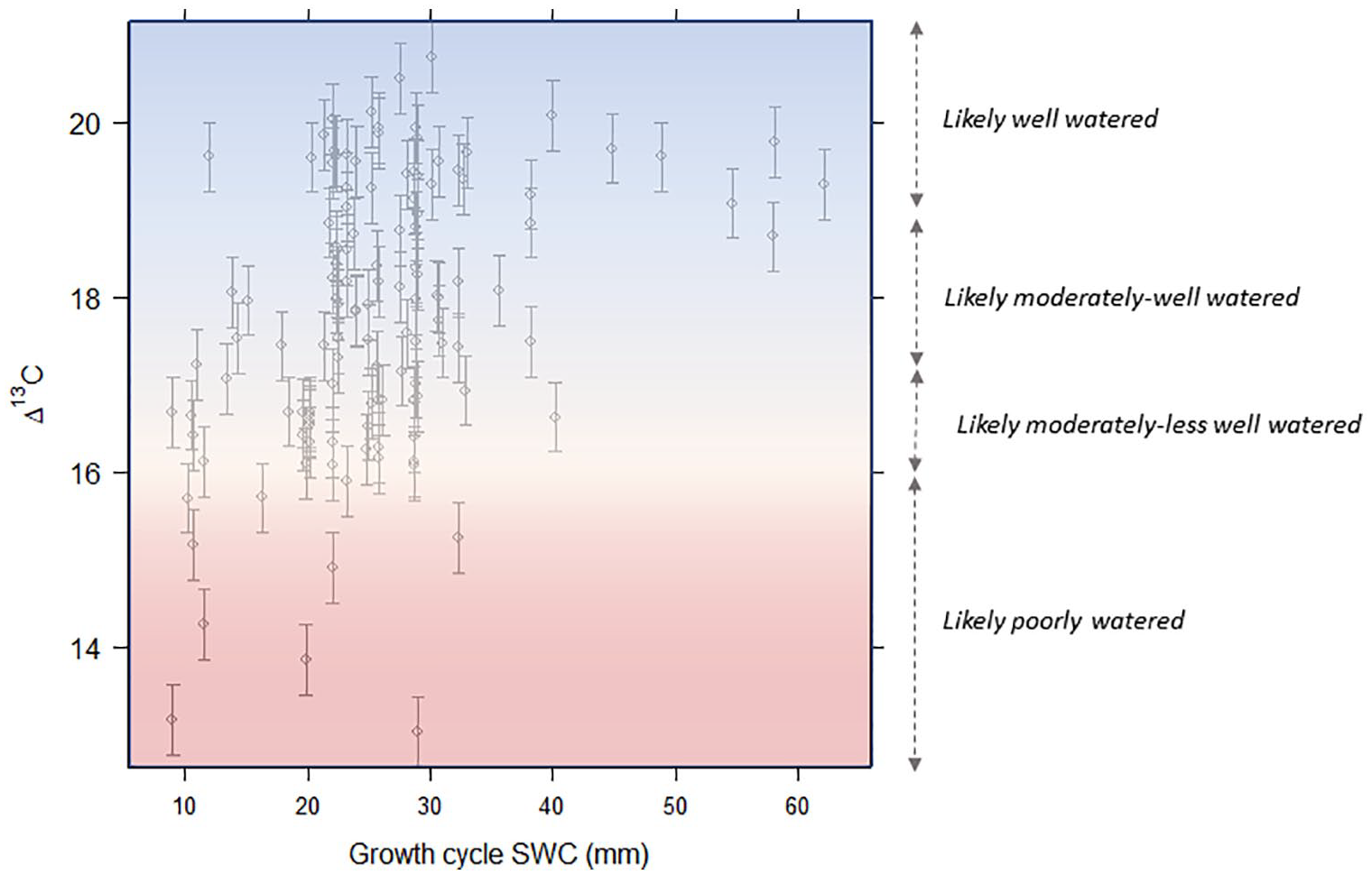
Proposed framework for the interpretation of archaeobotanical barley Δ¹³C in the greater Indus region, overlaid on a plot of modern barley Δ¹³C against climatic water availability and irrigation status. Climatic water availability is measured by the growing cycle (October to March) Soil Water Content (SWC, mm). The dotted lines and colour gradient emphasise that the values for demarcations between coarse bands of water status should not be treated as thresholds but simply useful marker points along a diffuse gradient of probabilities that a crop has been more or less well watered.

What are the broader implications for archaeological stable carbon isotope interpretation?

A key driver of this study was the need for empirical evidence to support archaeological applications of barley stable carbon isotope analysis interpretation in the greater Indus River Basin and analogous monsoonal climatic contexts. In addition to fulfilling this goal, our findings have important broader implications for archaeological Δ¹³C applications.

First, our findings support the broad transferability of water availability/Δ¹³C frameworks across a range of climatic regimes. Our proposed principles are significantly more conservative than, but not inconsistent with, frameworks previously proposed for Mediterranean regions. For example, on the basis of data from the Mediterranean and Levant, Wallace et al. (2013) proposed that barley Δ¹³C values >18.5‰ can be interpreted as indicative of well-watered barley, 17.5‰–18.5‰ as moderately watered, and <17.5‰ as poorly watered plants. We note that Wallace et al.’s (2013) values are approximately 0.4‰ offset (upwards) compared to ours, due to differences in the values used for modern δ¹³C_air - Wallace et al. (2013) used −8.00‰, whereas we used −8.42‰ and −8.44‰ as we had access to the more up-to-date δ¹³C_air estimates from Graven et al. (2017). Even after taking this difference into account, the thresholds proposed by Wallace et al. (2013) are broadly consistent with, even if much less conservative, than those proposed here. This consistency is not unexpected, but nevertheless represents an important explicit test of the transferability of principles across climatic contexts.

Second, this study adds to growing evidence that the degree of uncertainty inherent in crop Δ¹³C interpretation is much greater than commonly assumed. Our findings support the argument previously made by Wallace et al. (2013) and Flohr et al. (2011, 2019) that quantitative models relating Δ¹³C to water inputs are inappropriate, and demonstrate that in archaeological contexts, small differences in Δ¹³C either between sites or across periods cannot be confidently interpreted in terms of differences in moisture availability. In the context of barley, Wallace et al. (2013) suggested that any differences <0.5‰ should be disregarded. Even if some of the scatter in our data reflects our use of estimated rather than measured climatic water availability values, the sheer degree of scatter in the data presented here strongly suggest that an even more conservative approach is required. We further highlight the need to account for uncertainty introduced by δ¹³C_grain to Δ¹³C conversions (which we suggest are at least ±0.4‰), in addition to possible impacts from changes in atmospheric CO₂ concentration (Mora-González et al., 2019).

Third, our data provide further evidence that plant carbon isotope analysis has limited capacity to distinguish between intensities of irrigation in the archaeological record. We found considerable overlap in Δ¹³C in samples experiencing very different types and frequencies of irrigation. This observation adds to the findings of Flohr et al. (2019), who found overlapping Δ¹³C in barley receiving irrigation ranging from 40% to 120% of optimal water inputs in Jordan. Across a range of Mediterranean contexts, Wallace et al (2013) found that irrigation regimes recognised as distinct by farmers could not always be differentiated using Δ¹³C. Overall, this finding highlights that Δ¹³C cannot determine the detail of past water management regimes. An exception may be broad rainfed versus irrigated distinctions in arid zones – for example, Styring et al., 2016 found a marked difference between rainfed and oasis-irrigated barley in an arid (MAP <200 mm) area of Morocco, and in Jordan, Flohr et al. (2011) found a significant difference between rainfed and irrigated samples at sites receiving MAP <300 mm. Our data suggest that the ability to distinguish between rainfed/poorly-watered versus optimally-irrigated samples is likely to be strongest in areas receiving <400 mm rainfall/year: in this climatic band, rainfed or close-to-rainfed barley (low frequency sprinkler irrigation) has values typically <14.5‰, whereas all moderately to intensively irrigated barley has values over >16‰. In areas receiving > 400–450 mm/year, distinctions between un-irrigated, less intensively irrigated and more intensively irrigated barley appear difficult. This limitation has important implications for the ability of Δ¹³C analysis to contribute to debates about the existence and nature of irrigation in many archaeological contexts, including the Indus Civilisation.

Fourth, soil texture and mild to moderate salinity and water-logging appear unlikely to significantly confound the relationship between climatic water availability and Δ¹³C in an archaeological context. This observation is an important finding given that these soil qualities are often unknown and therefore difficult to control for analytically. Severe salinity and water-logging do result in very low Δ¹³C that could be mistakenly interpreted as a result of water shortage. However, other markers such as weed ecology and geoarchaeological proxies may assist in assessing the likelihood of any such confounding.

Finally, our study raises significant questions about the offset of 1‰ between two-row and six-row barley that has been applied in archaeological contexts (e.g. Styring et al., 2016; Wallace et al., 2015). We found no systematic difference between these two types and the ranges we propose above for broad categories of water status appear to apply equally to two- and six-row barley in NW India. Further investigation of whether and when any offset may be applicable is therefore required to support robust archaeological interpretation.

Conclusions

This study of modern barley stable carbon isotope values provides an empirically-supported platform for making inferences – however cautious – about past water status in NW India and climatically analogous monsoonal areas. Despite the high degree of noise, these data show that δ¹³C_grain is sensitive to the general climatic water balance, and they support water availability as the dominant single driver of δ¹³C_grain across the region. They suggest that inferred Δ¹³C values have capacity to identify both highly water-stressed and very well-watered conditions with a reasonable degree of confidence, even if inferences regarding irrigation regime, or moderate water status gradations appear difficult. Finally, within and beyond our study region, we highlight the significant uncertainty inherent in Δ¹³C interpretation, and recommend that isotopic interpretations are supported wherever possible by complementary evidence from weed ecology, geoarchaeological and palaeoecological data.

Supplemental Material

sj-pdf-1-hol-10.1177_0959683621994649 – Supplemental material for Crop water status from plant stable carbon isotope values: A test case for monsoonal climates

Supplemental material, sj-pdf-1-hol-10.1177_0959683621994649 for Crop water status from plant stable carbon isotope values: A test case for monsoonal climates by Penelope J Jones, Tamsin C O’Connell, Martin K Jones, RN Singh and Cameron A Petrie in The Holocene

Supplemental Material

sj-xlsx-1-hol-10.1177_0959683621994649 – Supplemental material for Crop water status from plant stable carbon isotope values: A test case for monsoonal climates

Supplemental material, sj-xlsx-1-hol-10.1177_0959683621994649 for Crop water status from plant stable carbon isotope values: A test case for monsoonal climates by Penelope J Jones, Tamsin C O’Connell, Martin K Jones, RN Singh and Cameron A Petrie in The Holocene

Supplemental Material

sj-xlsx-2-hol-10.1177_0959683621994649 – Supplemental material for Crop water status from plant stable carbon isotope values: A test case for monsoonal climates

Supplemental material, sj-xlsx-2-hol-10.1177_0959683621994649 for Crop water status from plant stable carbon isotope values: A test case for monsoonal climates by Penelope J Jones, Tamsin C O’Connell, Martin K Jones, RN Singh and Cameron A Petrie in The Holocene

Footnotes

Acknowledgements

The authors thank the barley producers of Haryana and Rajasthan for permission to access their fields and for providing cultivation histories. Appu Singh (MD University Rohtak) and Amit Ranjan (Banaras Hindu University) made this study possible as translators and field guides. We would also like to thank the Department of AIHC and Archaeology at Banaras Hindu University for their logistical support. At the University of Cambridge, we are grateful to Catherine Kneale and James Rolfe for their help with isotopic analysis, Chris Rolfe for allowing access to facilities and Louise Butterworth and Samantha Smith for technical support. We would like to thank Howard Griffiths, Nick Owen, Emma Lightfoot and Jennifer Bates for useful discussions and advice. AK Pandey provided valuable support in the field and we thank David Redhouse and Ian Hitchman for IT support. No aspect of the broader archaeological study that this work helped inform would have been possible without excavation and export permission from the Archaeological Survey of India.

Funding

The author(s) disclosed receipt of the following financial support for the research, authorship, and/or publication of this article: This paper developed out of research conducted for the Land, Water and Settlement and TwoRains projects, which are both collaborations between Banaras Hindu University and the University of Cambridge investigating human–environment relations in northwest India. The Land, Water and Settlement project was primarily funded by a Standard Award from the UK India Education and Research Initiative (UKIERI) under the title ‘From the collapse of Harappan urbanism to the rise of the great Early Historic cities: Investigating the cultural and geographical transformation of northwest India between 2000 and 300 BC’. The TwoRains project is funded by the European Research Council under the European Union’s Horizon 2020 research and innovation program [grant number 648609]. This specific study received additional funding from the Geographical Club, INTACH-UK and the European Research Council project Food Globalization in Prehistory [grant number GA249642]. PJ Jones’ overall doctoral study was funded by the Rae and Edith Bennett Travelling Scholarship.

ORCID iD

Penelope J Jones

Supplemental material

Supplemental material for this article is available online.

References

Aguilera

Espinar

Ferrio

, et al. (2009) A map of autumn precipitation for the third millennium BP in the Eastern Iberian Peninsula from charcoal carbon isotopes. Journal of Geochemical Exploration 102(3): 157–165.

Aguilera

Ferrio

Araus

, et al. (2011) Climate at the onset of western Mediterranean agriculture expansion: Evidence from stable isotopes of sub-fossil oak tree rings in Spain. Palaeogeography, Palaeoclimatology, Palaeoecology 299(3–4): 541–551.

Aguilera

Ferrio

Pérez

, et al. (2012) Holocene changes in precipitation seasonality in the western Mediterranean basin: A multi-species approach using δ13C of archaeobotanical remains. Journal of Quaternary Science 27(2): 192–202.

Anyia

Slaski

Nyachiro

, et al. (2007) Relationship of carbon isotope discrimination to water use efficiency and productivity of barley under field and greenhouse conditions. Journal of Agronomy and Crop Science 193(5): 313–323.

Araus

Febrero

Buxo

, et al. (1997) Identification of ancient irrigation practices based on the carbon isotope discrimination of plant seeds: A case study from the South-East Iberian Peninsula. Journal of Archaeological Science 24(8): 729–740.

Araus

Febrero

Catala

, et al. (1999) Crop water availability in early agriculture: Evidence from carbon isotope discrimination of seeds from a tenth millennium BP site on the Euphrates. Global Change Biology 5(2): 201–212.

Araus

Ferrio

Voltas

, et al. (2014) Agronomic conditions and crop evolution in ancient Near East agriculture. Nature Communications 5: 3953.

Araus

Slafer

Romagosa

, et al. (2001) Estimated wheat yields during the emergence of agriculture based on the carbon isotope discrimination of grains: Evidence from a 10th millenium BP site on the Euphrates. Journal of Archaeological Science 28: 341–350.

Bates

(2016) Social Organisation and Change in Bronze Age South Asia: A Multi-Proxy Approach to Urbanisation, Deurbanisation and Village Life through Phytolith and Macrobotanical Analysis. Cambridge: University of Cambridge.

10.

Bogaard

Hodgson

Nitsch

, et al. (2016) Combining functional weed ecology and crop stable isotope ratios to identify cultivation intensity: A comparison of cereal production regimes in Haute Provence, France and Asturias, Spain. Vegetation History and Archaeobotany 25(1): 57–73.

11.

Brugnoli

Farquhar

(2000) Photosynthetic fractionation of carbon isotopes. In: Leegood

Sharkey

von Caemmerer

(eds) Photosynthesis. Dordrecht: Springer Netherlands, pp.399–434.

12.

Cernusak

Ubierna

Winter

, et al. (2013) Environmental and physiological determinants of carbon isotope discrimination in terrestrial plants. The New Phytologist 200(4): 950–965.

13.

Diefendorf

Mueller

Wing

, et al. (2010) Global patterns in leaf ¹³C discrimination and implications for studies of past and future climate. Proceedings of the National Academy of Sciences of the United States of America 107(13): 5738–5743.

14.

Farquhar

Ehleringer

Hubick

(1989) Carbon isotope discrimination and photosynthesis. Annual Review of Plant Physiology and Plant Molecular Biology 40(1): 503–537.

15.

Farquhar

O’Leary

Berry

(1982) On the relationship between carbon isotope discrimination and the inter-cellular carbon-dioxide concentration in leaves. Australian Journal of Plant Physiology 9: 121–137.

16.

Ferrio

Araus

Buxó

, et al. (2005) Water management practices and climate in ancient agriculture: Inferences from the stable isotope composition of archaeobotanical remains. Vegetation History and Archaeobotany 14(4): 510–517.

17.

Ferrio

Voltas

(2005) Carbon and oxygen isotope ratios in wood constituents of Pinus halepensis as indicators of precipitation, temperature and vapour pressure deficit. Tellus 57B: 164–173.

18.

Fiorentino

Caracuta

Casiello

, et al. (2012) Studying ancient crop provenance: Implications from δ(13)C and δ(15)N values of charred barley in a Middle Bronze Age silo at Ebla (NW Syria). Rapid Communications in Mass Spectrometry 26(3): 327–335.

19.

Flohr

Fleitmann

Matthews

, et al. (2016) Evidence of resilience to past climate change in Southwest Asia: Early farming communities and the 9.2 and 8.2 ka events. Quaternary Science Reviews 136: 23–39.

20.

Flohr

Jenkins

Williams

HRS

, et al. (2019) What can crop stable isotopes ever do for us? An experimental perspective on using cereal carbon stable isotope values for reconstructing water availability in semi-arid and arid environments. Vegetation History and Archaeobotany 28(5): 497–512.

21.

Flohr

Muldner

Jenkins

(2011) Carbon stable isotope analysis of cereal remains as a way to reconstruct water availability: Preliminary results. Water History 3: 121–144.

22.

Fox

Weisberg

(2011) An {R} Companion to Applied Regression, 2nd edn. Thousand Oaks, CA: Sage.

23.

Graven

Allison

Etheridge

, et al. (2017) Compiled records of carbon isotopes in atmospheric CO₂ for historical simulations in CMIP6. Geoscientific Model Development Discussions 10: 4405–4417.

24.

Hare

Loftus

Jeffrey

, et al. (2018) Atmospheric CO₂ effect on stable carbon isotope composition of terrestrial fossil archives. Nature Communications 9: 252.

25.

Jiang

Roche

Hole

(2006) Carbon isotope discrimination of two-rowed and six-rowed barley genotypes under irrigated and non-irrigated field conditions. Canadian Journal of Plant Science 86: 433–441.

26.

Kohn

(2010) Carbon isotope compositions of terrestrial C3 plants as indicators of (paleo)ecology and (paleo)climate. Proceedings of the National Academy of Sciences of the United States of America 107(46): 19691–19695.

27.

Lightfoot

Stevens

(2012) Stable isotope investigations of charred barley (Hordeum vulgare) and wheat (Triticum spelta) grains from Danebury Hillfort: Implications for palaeodietary reconstructions. Journal of Archaeological Science 39(3): 656–662.

28.

Liu

Lister

Zhao

, et al. (2017) Journey to the east: Diverse routes and variable flowering times for wheat and barley en route to prehistoric China. PLoS One 12(11): e0209518.

29.

Masi

Sadori

Balossi Restelli

, et al. (2013) Stable carbon isotope analysis as a crop management indicator at Arslantepe (Malatya, Turkey) during the Late Chalcolithic and Early Bronze Age. Vegetation History and Archaeobotany 23(6): 751–760.

30.

Miller

(2015) Surplus in the Indus civilization: Agricultural choices, social relations, political effects. In: Morehart

De Lucia

(eds) Surplus. Boulder, CO: University Press of Colorado.

31.

Mora-González

Fernandes

Cortés

, et al. (2019) Reporting atmospheric CO₂ pressure corrected results of stable carbon isotope analyses of cereals remains from the archaeological site of Peñalosa (SE Iberian Peninsula): Agricultural and social implications. Archaeologial and Anthropological Sciences 11: 1995–2005.

32.

O’Leary

(1988) Carbon isotopes in photosynthesis. BioScience 38(5): 328–336.

33.

Peters

(2015) userfriendlyscience: Quantitative analysis made accessible. R package version 0.3-0. Available at: https://CRAN.R-project.org/package=userfriendlyscience (accessed 25 February 2015).

34.

Petrie

Singh

French

CAI

, et al. (2017) Adaptation to variable environments, resilience to climate change. Current Anthropology 58(1): 1–30.

35.

Pokharia

Kharakwal

Srivastava

(2013) Archaeobotanical evidence of millets in the Indian subcontinent with some observations on their role in the Indus civilization. Journal of Archaeological Science 42: 442–455.

36.

R Development Core Team (2018) R: A Language and Environment for Statistical Computing. 3.4.4. Vienna: R Foundation for Statistical Computing.

37.

Riehl

Bryson

Pustovoytov

(2008) Changing growing conditions for crops during the Near Eastern Bronze Age (3000–1200 BC): The stable carbon isotope evidence. Journal of Archaeological Science 35(4): 1011–1022.

38.

Riehl

Pustovoytov

Weippert

, et al. (2014) Drought stress variability in ancient Near Eastern agricultural systems evidenced by δ13C in barley grain. Proceedings of the National Academy of Sciences of the United States of America 111(34): 12348–12353.

39.

Saxton

Rawls

(2006) Soil water characteristic estimates by texture and organic matter for hydrologic solutions. Soil Science Society of America Journal 70(5): 1569–1578.

40.

Sperry

Hacke

(2002) Desert shrub water relations with respect to soil and plant functional type characteristics. Functional Ecology 16(3): 367–378.

41.

Styring

Ater

Hmimsa

, et al. (2016) Disentangling the effect of farming practice from aridity on crop stable isotope values: A present-day model from Morocco and its application to early farming sites in the eastern Mediterranean. The Anthropocene Review 3: 2–22.

42.

Styring

Charles

Fantone

, et al. (2017) Isotope evidence for agricultural extensification reveals how the world’s first cities were fed. Nature Plants 3: 17076.

43.

Szpak

Metcalfe

Macdonald

(2017) Best practices for calibrating and reporting stable isotope measurements in archaeology. Journal of Archaeological Science: Reports 13: 609–616.

44.

Tieszen

(1991) Natural variations in the carbon isotope values of plants: Implications for archaeology, ecology, and paleoecology. Journal of Archaeological Science 18(3): 227–248.

45.

Trabucco

Zomer

(2010) Global soil water balance geospatial database. Available at: https://cgiarcsi.community/data/global-high-resolution-soil-water-balance/.

46.

Trabucco

Zomer

Bossio

, et al. (2008) Climate change mitigation through afforestation/reforestation: A global analysis of hydrologic impacts with four case studies. Agriculture, Ecosystems & Environment 126(1–2): 81–97.

47.

Vaiglova

Bogaard

Collins

, et al. (2014) An integrated stable isotope study of plants and animals from Kouphovouno, southern Greece: A new look at Neolithic farming. Journal of Archaeological Science 42: 201–215.

48.

Voltas

Romagosa

Lafarga

, et al. (1999) Genotype by environment interaction for grain yield and carbon isotope discrimination of barley in Mediterranean Spain. Australian Journal of Agricultural Research 50(7): 1263.

49.

Wallace

Jones

Charles

, et al. (2013) Stable carbon isotope analysis as a direct means of inferring crop water status and water management practices. World Archaeology 45(3): 388–409.

50.

Wallace

Jones

Charles

, et al. (2015) Stable carbon isotope evidence for Neolithic and Bronze Age crop water management in the eastern Mediterranean and southwest Asia. PloS One 10(6): e0127085.

51.

WorldClim (2012) WorldClim – global climate data. ERSI grids for mean, maximum and minimum temperature, precipitation and bioclimatic variables (30 arc-seconds). Available at: https://www.worldclim.org/data/index.html (accessed 25 May 2015).

Supplementary Material

Please find the following supplemental material available below.

For Open Access articles published under a Creative Commons License, all supplemental material carries the same license as the article it is associated with.

For non-Open Access articles published, all supplemental material carries a non-exclusive license, and permission requests for re-use of supplemental material or any part of supplemental material shall be sent directly to the copyright owner as specified in the copyright notice associated with the article.

0.00 MB

1.36 MB

0.02 MB

0.06 MB

Crop water status from plant stable carbon isotope values: A test case for monsoonal climates

Abstract

Keywords

Introduction

Principles of plant stable carbon isotopes as a water proxy

Support for archaeological applications

Material and methods

Sample collection

Laboratory protocol and mass spectrometry

Environmental variable estimation

Statistical analysis

Conversion to Δ13C

Results

The relationship between δ13Cgrain and climatic water availability

Effects of irrigation, soil texture, waterlogging, salinity and sub-species

Irrigation type

Irrigation frequency

Soil properties

Waterlogging and salinity

Six-row versus two-row sub-species

Conversion to Δ13C

Discussion

What is the relationship between δ13Cgrain and climatic water availability?

How do irrigation, soil texture, waterlogging, salinity and sub-species affect this relationship?

Irrigation

Soil texture

Salinity and waterlogging

Six-row versus two-row sub-species

What are the implications for archaeological application in monsoonal NW India?

What are the broader implications for archaeological stable carbon isotope interpretation?

Conclusions

Supplemental Material

sj-pdf-1-hol-10.1177_0959683621994649 – Supplemental material for Crop water status from plant stable carbon isotope values: A test case for monsoonal climates

Supplemental Material

sj-xlsx-1-hol-10.1177_0959683621994649 – Supplemental material for Crop water status from plant stable carbon isotope values: A test case for monsoonal climates

Supplemental Material

sj-xlsx-2-hol-10.1177_0959683621994649 – Supplemental material for Crop water status from plant stable carbon isotope values: A test case for monsoonal climates

Footnotes

Acknowledgements

Funding

ORCID iD

Supplemental material

References

Supplementary Material

Conversion to Δ¹³C

The relationship between δ¹³C_grain and climatic water availability

Conversion to Δ¹³C

What is the relationship between δ¹³C_grain and climatic water availability?