
Abstract
Pollen productivity estimates (PPEs) are a key parameter for quantitative land-cover reconstructions from pollen data. PPEs are commonly estimated using modern pollen-vegetation data sets and the extended R-value (ERV) model. Prominent discrepancies in the existing studies question the reliability of the approach. We here propose an implementation of the ERV model in the R environment for statistical computing, which allows for simplified application and testing. Using simulated pollen-vegetation data sets, we explore sensitivity of ERV application to (1) number of sites, (2) vegetation structure, (3) basin size, (4) noise in the data, and (5) dispersal model selection. The simulations show that noise in the (pollen) data and dispersal model selection are critical factors in ERV application. Pollen count errors imply prominent PPE errors mainly for taxa with low counts, usually low pollen producers. Applied with an unsuited dispersal model, ERV tends to produce wrong PPEs for additional taxa. In a comparison of the still widely applied Prentice model and a Lagrangian stochastic model (LSM), errors are highest for taxa with high and low fall speed of pollen. The errors reflect the too high influence of fall speed in the Prentice model. ERV studies often use local scale pollen data from for example, moss polsters. Describing pollen dispersal on his local scale is particularly complex due to a range of disturbing factors, including differential release height. Considering the importance of the dispersal model in the approach, and the very large uncertainties in dispersal on short distance, we advise to carry out ERV studies with pollen data from open areas or basins that lack local pollen deposition of the taxa of interest.
Keywords
Introduction
Pollen based land-cover reconstructions provide long-term observations of past vegetation, which are valuable in various fields, including ecology, nature conservation, archaeology, and climate science. The interpretation of pollen data is far from simple, however. Mainly the fact that plants produce pollen in very different amounts introduces bias in pollen values, with strong pollen producers being over-represented and weak pollen producers being under-represented. Interpretation is further complicated by different dispersal of small and large pollen grains. The presence of bias in pollen data is known since the inception of the field, and experienced palynologist try to account for it when interpreting pollen data. With the advent of methods such as LRA (including REVEALS and LOVE, Sugita, 2007a, 2007b), Marco Polo (Mrotzek et al., 2017), MSA (Bunting and Middleton, 2009), and EDA (Theuerkauf and Couwenberg, 2017) more objective quantitative reconstructions of past vegetation cover became feasible. Yet, widespread application is still hampered by the limited availability of the necessary correction factors, namely pollen productivity estimates (PPEs or RPPs).
PPEs are usually estimated by calibration of the pollen-vegetation relationship, that is, by relating modern pollen deposition in a set of sample sites to modern vegetation composition in the surrounding of each of these respective sites. One way to calibrate is to use pollen samples from larger lakes (or peatlands) with prevailing regional pollen deposition, that is, samples that represent regional scale vegetation composition. Using this type of “regional” pollen counts requires estimating plant abundances on a large scale to arrive at good PPE estimates, a “large lake” approach will require plant cover data in a 30–50 km radius around each sample site to arrive at robust PPEs. PPEs in this case can be calculated with iterative approaches (Fang et al., 2019; Theuerkauf et al., 2013) or by using the inverse REVEALS model (Kuneš et al., 2019). The most critical step in the calculations is the appropriate distance weighting of the plant abundance data. Or, in other words, using the right pollen dispersal model (Theuerkauf et al., 2013). A pollen dispersal model is needed to account for the fact that plants growing in greater distance from a sample site contribute less pollen than those growing nearby; dispersal may also differ between plant taxa. Only if the chosen dispersal model reflects true pollen dispersal in the landscape well, the resulting PPEs will indeed represent pollen productivity of each taxon.
More often, PPEs are estimated with a set of pollen samples from small lakes, moss pollsters, or pollen traps. Commonly, the extended R-value (ERV) model is used to calibrate pollen counts and vegetation cover (Parsons and Prentice, 1981, Prentice and Parsons, 1983, Sugita, 1994). The main advantage of this approach is that it reduces the necessary vegetation mapping. Pollen records from small wet (forest) depressions, moss pollsters, and pollen traps include both (extra)local and regional pollen deposition. The ERV model assumes that regional pollen deposition is similar at all pollen sample sites. The assumption is that far-away vegetation cover is similar for all pollen sampling sites and that regional pollen influx from far-away is equal for all sites, Following this assumption, mapping is only necessary for the nearby vegetation contributing the (extra)local pollen deposition, in practice usually 1–2 km distance around each pollen sampling site. Moreover, many herb taxa are more commonly recorded in small sample sites than in large lakes, so that the ERV approach with pollen data from small sites appears better suited to produce PPEs also for a range of herbal taxa. So far, the ERV model has been applied in more than 40 studies, mainly from Europe and China.
ERV application is not without problems, however. Data compilations from Central and Northern Europe (Broström et al., 2008, Mazier et al., 2012) and temperate China (Li et al., 2018) show large and yet mostly unexplained variations in the presented PPEs. The variations may relate to methodological issues, with quantification of plant abundances apparently being a particularly critical step (Bunting et al., 2013, Li et al., 2018). Also sample selection, sample type, vegetation structure, and ERV model selection may play a role (Li et al., 2018). The variations may also represent true differences in pollen productivity related to environmental and biological parameters, such as climate, vegetation structure, and species composition, yet such relationships are rarely identified (Matthias et al., 2012). Overall, a better understanding of the pitfalls of the ERV approach is necessary to arrive at more robust results.
Simulation studies are one option to explore these pitfalls. Using simulations, Sugita (1994) showed the importance of vegetation patch size and basin size in ERV modeling. Other factors, such as dispersal model selection and error in pollen data, have not yet been studied. To allow for flexibility in ERV application as well as for simulation studies, we have implemented the ERV model in the R environment for statistical computing (R Core Team, 2020). With this tool, we in the following test the effect of five parameters: (1) number of sites, (2) vegetation structure, (3) basin size, (4) noise in the input data, and (5) dispersal model selection.
At first, we introduce the rationale of our ERV implementation.
Theory behind the ERV model
Attempts to estimate correction factors from surface pollen data have a long history (e.g. Jonassen, 1950; Müller, 1937; Steinberg, 1944; Tsukada, 1958). Davis (1963) formalized the approach in the R-value model, with the R-value defined as the ratio of the pollen percentage value in a surface sample and the proportionate plant abundance in the surrounding vegetation. The key challenge is to estimate actual plant abundances in a suitable and effective way. Airborne pollen is easily transported over 10s of km or farther, which means that pollen source areas are very large and usually too large to be mapped. To account for pollen transported over long-distances to the sample site, that is, from beyond the mapped area, Parsons and Prentice (1981) and Prentice and Parsons (1983) proposed to add a background component in what became the extended R-value model (ERV model). The fundamental assumption is that this background component is the same at each of the studied sites. Prentice and Parsons (1983) propose two ways to express that background component, either as “a constant background pollen percentage for each taxon” (model 1) or “as a constant proportion of total forest volume (or whatever measure of abundance is being used)” (model 2, Parsons and Prentice, 1981). Model 3, added by Sugita (1994), assumes a constant absolute amount of background pollen deposition for each taxon at all sites.
Moreover, Sugita (1994) suggests using distance weighted plant abundances instead of simple vegetation proportions in order to account for dispersal effects in pollen data. There are two overlapping dispersal effects. First, plants growing in the vicinity of a site contribute more pollen than those farther away. Secondly, dispersal distances may differ between plant taxa, depending on the size and fall speed of their pollen. Distance weighting aims to compensate for both effects by using a pollen dispersal model. If the dispersal bias can be removed, the correction factors would represent over-/under-representation related to differences in pollen productivity alone. In other words, (only) when using suitable distance weighting, the resulting correction factors represent relative pollen productivities of plant taxa.
Like the existing models, our implementation of the ERV model starts with the fundamental assumption that pollen deposition D of taxon i at a site k can be expressed as “local” pollen deposition (or pollen loading, sensu Sugita, 1994) PLlocal plus background pollen deposition PLbackground (equation (1)). Local pollen arrives from the area for which mapped vegetation data is available, background pollen from beyond.

Pollen deposition in general can be expressed as the result of pollen production in the source area and pollen dispersal to the study site. For each taxon i of the “local” vegetation at each site k, the “local” pollen deposition can be expressed as distance weighted plant abundance dwpa multiplied by pollen productivity α (equation (2)).

Equation (2) can be written in terms of relative pollen deposition by dividing pollen deposition of taxon i at site k with summed-up pollen deposition of all taxa at this site (equation (3)), similar to ERV model 3 from Sugita, 1994).
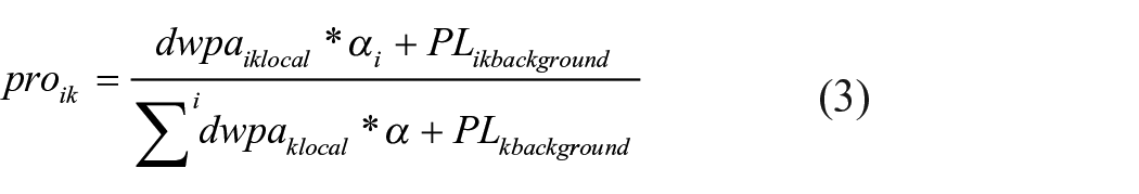
We aim to determine α from pollen percentages and distance-weighted plant abundances. Equation (3) does not allow us to do so directly, because it includes background pollen deposition of each taxon as another unknown variable. Yet, with pollen and vegetation data from a set of sites, we can approximate α using numerical optimization, at least under the assumption that the background component for the individual taxa is the same across all sites. We can assume random values for α and PLbackground for each individual taxon and use equation (3) to calculate relative pollen deposition (right-hand side of equation (3)). We compare this modeled pollen deposition to observed pollen deposition (left-hand side of equation (3)) and using an optimization algorithm find those values for α and PLbackground, that give the best match between the modeled and observed pollen deposition for each taxon and each site.
As a modification to ERV model 3, we express the background component not as abstract pollen loading but also as pollen productivity α multiplied by the distance weighted, “regional” plant abundance for each taxon (equation (4)). To clearly highlight this modification of model 3, we name this version ERV model 4. If available, “regional” abundances can be compared to true abundances, for example from forest inventories, allowing for a validation of the ERV application.
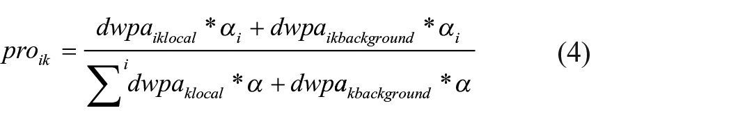
In our implementation, we arrive at best estimates for α and dwparegional by minimizing the squared chord distance between observed (left-hand side of equation (4)) and modeled pollen percentages (right-hand side of equation (4)). For optimization we use the conjugate-gradient algorithms with the “optim” function from the {stats} package in R. Tests have shown more accurate results than with the Nelder-Mead method, which is used in the ERV program(s) of Shinya Sugita. Our approach does not a priori set a reference taxon. All α values are allowed to permutate in a user-defined corridor (e.g. 0.01–20) and the reference taxon to calculate relative values, that is, PPEs, is chosen later. The total cover of regional vegetation is assumed to be 100% as a standard, but it may be set to lower values to allow for non-pollen producing areas. For evaluation, we compare modeled with observed pollen percentages (right-hand side with left-hand side of equation (4)). This relationship should in theory be linear. Simulations, even with noisy pollen data, indeed show linearity (Figure 1). ERV models 1–3 use different measures for evaluation. With ERV1 we look at scatterplots of adjusted vegetation proportion versus pollen proportion; with ERV2 at vegetation proportions versus adjusted pollen proportions; with ERV3 at relative pollen loadings versus absolute vegetation. Using simulated data, also model 2 and 3, but not model 1, show linear relationships (Figure 1).
Diagnostic scatter plots for Alnus from ERV application with model 1–4 using vegetation composition in different radii as input and deeming vegetation beyond this radius “regional” (see grayscale legend). Model 1–3 calculated with the ERV.Analysis.v2.5.3 program of Shinya Sugita. Model 4 calculated with the “ERVinR” function. The same simulated data set has been used in all four cases (basin size = 10 m, noise added in counts, 30 sites). The data set has been created and ERV has been applied with the Lagrangian-Stochastic-model for pollen dispersal (LSM).
Testing
Preparation of simulated data sets
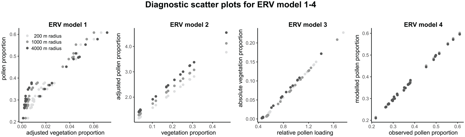
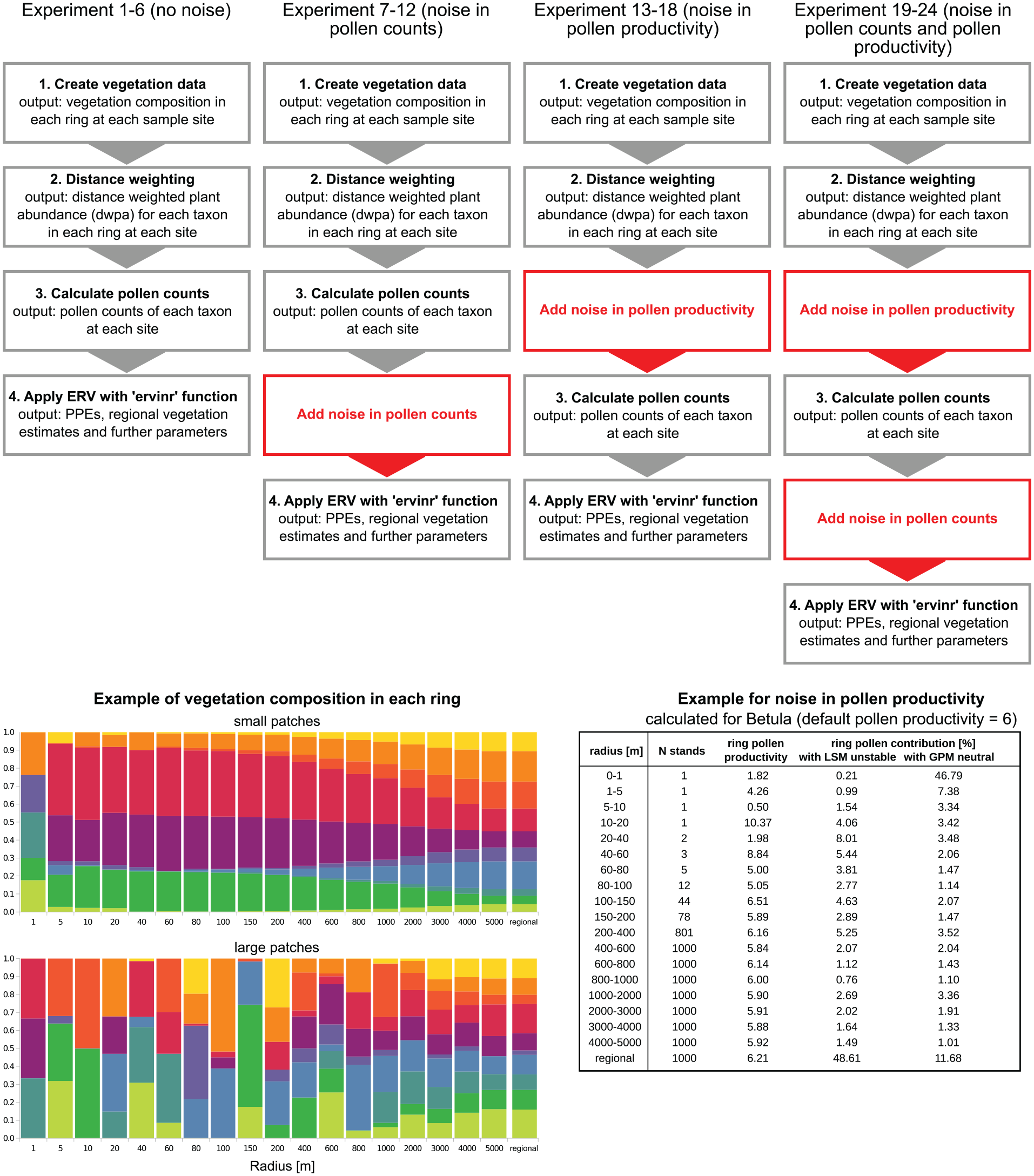
We tested the ERV approach using simulated pollen-vegetation data sets. Each data set includes a number of sites (10–50). The data sets are created in a way that vegetation within 5 km distance from the center of each site is different (=“local vegetation”), while vegetation beyond 5 km is uniform (=“regional vegetation”). The local part is composed of consecutive rings with increasing ring width (Figure 2). Each data set is created in the following steps:
Create vegetation data: First, regional vegetation composition is set to random values (sum = 100%). Then, vegetation composition in the smallest ring around each site is set to random values. To mimic real-world conditions, abundances in the smallest ring are created so that only a few taxa are dominant while others are absent (sum = 100%). This is achieved by cutting of smaller values and recalculating the rest to 100% cover. Vegetation composition in all further local rings is calculated in two steps. First, preliminary abundances of each taxon and each ring are calculated by interpolating linearly between abundances in the innermost ring and regional abundances. These values are then altered by a random component, which decreases with ring size. We use a small random component to simulate a setting with small vegetation patches (experiment 1, 3, . . ., 23) and a large random component to simulate a setting with large vegetation patches (experiment 2, 4, . . ., 24, see below).
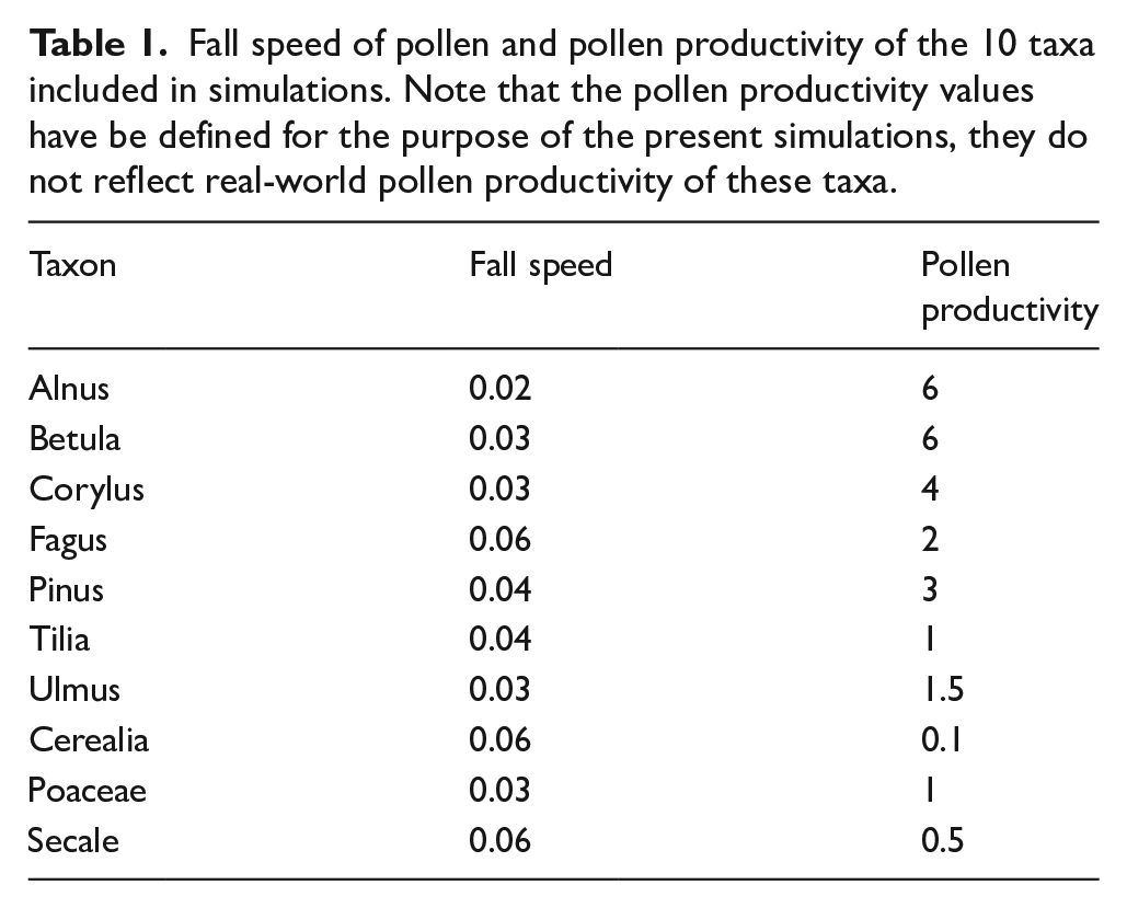
Apply distance weighting: Distance weighted plant abundances (dwpa) are calculated by multiplying the cover of each taxon in each ring, as well as in the regional vegetation, by a respective distance weighting factor. Distance weighting factors are calculated with the Lagrangian-Stochastic-model for pollen dispersal (LSM) from Kuparinen et al. (2007), adjusted to unstable atmospheric conditions and using fall speed values for the individual taxa (Table 1). Only in the experiments that test effects of dispersal model selection, we calculated distance weighting factors also with a Gaussian plume model.
Calculate pollen counts: To first calculate pollen deposition of each taxon at each site, the dwpa values of that taxon in each ring, as well as in the regional vegetation, were multiplied with the relative pollen productivity of that taxon (Table 1) and summed up. The pollen count of each taxon is then calculated as the pollen deposition of the taxon divided by total pollen deposition, multiplied with 1000, and rounded to zero digits. In this way we arrive at a pollen sum of 1000 pollen grains.
Top: The main steps of our simulation approach for experiments with and without noise in pollen counts and pollen productivity. The details of each step are described in the text. Bottom left: Example for vegetation composition in each ring for one study site with either small or large ring-to-ring variation in local vegetation composition, representing small or large patches. Bottom right: Example for noise in pollen productivity calculated for Betula (default pollen productivity = 6). For each ring, the cover of Betula (in m²) is divided by 25 to calculate the number N of 25 m2 stands (minimum number of stands = 1, maximum = 1000). For each ring, N random pollen productivity values are drawn (for Betula between 0 and 12). The mean of these N values is then the pollen productivity for this ring.
Fall speed of pollen and pollen productivity of the 10 taxa included in simulations. Note that the pollen productivity values have be defined for the purpose of the present simulations, they do not reflect real-world pollen productivity of these taxa.
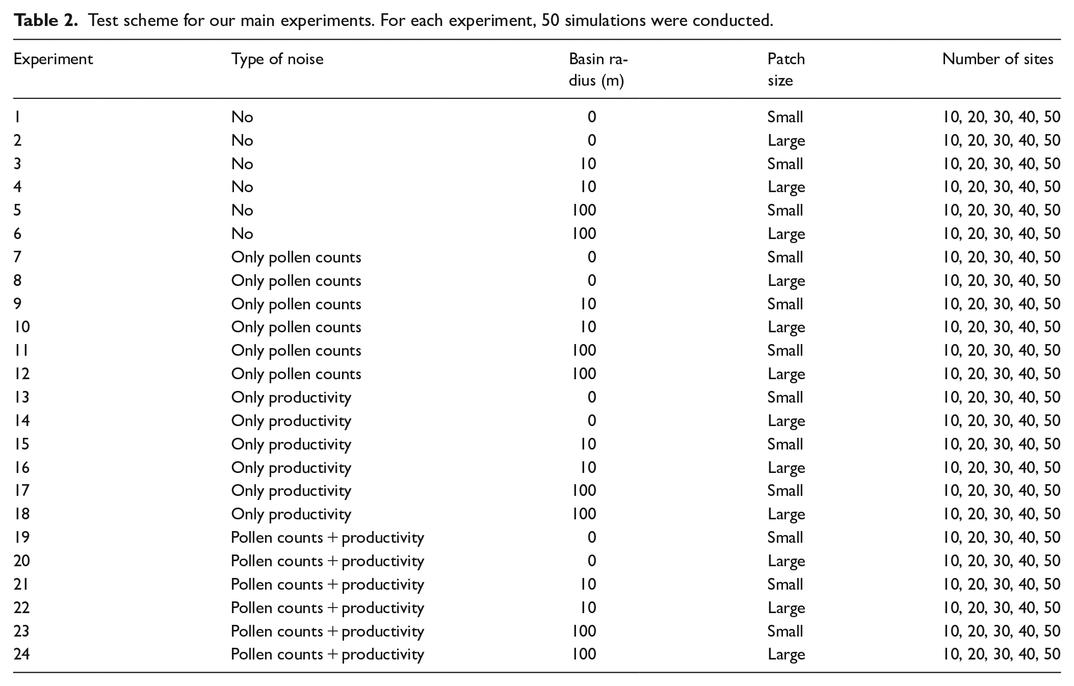
With these data sets, we test the influence of five parameters on ERV application: (1) number of sites, (2) vegetation patch size, (3) basin size, (4) noise in the data set, and (5) dispersal model selection (Table 2). To account for the number of sites, we created data sets with 10, 20, 30, 40, and 50 sites. To account for basin size, we created data sets with a basin radius of 0, 10, and 100 m. We did not test for larger basin sizes because the ERV model is not suited for pollen data from large sites with prevailing regional pollen deposition.
Test scheme for our main experiments. For each experiment, 50 simulations were conducted.
To account for vegetation structure, we created two types of data sets that mimic small and large vegetation patches (Figure 2). In case of small, homogeneously arranged patches, the added random component is small so that abundances change smoothly from the inner to the outermost rings. These simulations mimic the vegetation pattern of a largely homogenous, mixed forest with patches of ~10 in diameter. In case of larger patches, the added random component is large so that abundances change more strongly from ring to ring, particularly in the smaller rings. These simulations mimic the vegetation pattern of an arable landscape with patches from 10 to 1000 m in diameter (or larger).
To explore effects of inaccuracies in pollen counts and pollen productivity, we run experiments first without and then with two levels of inaccuracy. The first level adds noise to the virtual pollen counts: Instead of using the true, simulated pollen counts, we draw a new pollen sample with a default sum of 1000 pollen for each site with the true pollen composition as a basis. As in real pollen samples, the size of errors depends on the abundance of a pollen type, that is, errors are highest for rare pollen types (Mosimann, 1965). For example, if one counts 1000 pollen grains from a sample with exactly 1% Cerealia pollen, then chances are high that the final count does not include the expected 10 (=1%) but for example, only 5 or even 20 Cerealia pollen grains. To draw pollen samples we used multinomial drawing with the R-function “rmultinom” (with number of samples “n” = 1, number of objects “size” = pollensum, composition of the population “prob” = true pollen composition).
The second level of inaccuracy adds noise to pollen productivity. This type of noise simulates variation in the pollen productivity between single specimens (or small stands) of one and the same taxon, which in reality would occur for example due to differences in genetics, health, age, or site conditions. In the simulations, we assume that pollen productivity for a taxon is uniform for stands of 25 m2, which is about the basal area of a single tree. In effect we are thus mimicking differential pollen production among single trees. For each 25 m2 stand, pollen productivity is estimated by drawing a random value between 0 and 2 times the true pollen productivity. Then, for each ring the mean of these random productivities is calculated for each taxon. Hence, for each taxon and ring we arrive at a unique pollen productivity value. Logically, this type of noise causes the largest offset from the mean in the smallest rings with only a low number of stands.
As the “taxa” in our simulations are simulated entities, not existing plants, we use a normal font.
The combination of four types of noise, three types of basin size, and two types of vegetation structure gives a total of 24 experiments (Table 2). Each experiment was run with 10, 20, 30, 40, and 50 sites. To explore stability of the ERV applications, we for each experiment repeated simulations 50 times (=50 simulations). Each simulation starts with a newly created pollen-vegetation data set.
Application of the “ERVinR” function starts with only the innermost ring, further rings are then added successively. By default, “ERVinR” was applied with the LSM, adjusted for unstable atmospheric conditions. The resulting PPEs and regional cover estimates are compared with the actual, true values that were used to synthesize the virtual datasets and deviations are expressed as root-median-squared error (rmse).
Testing effects of dispersal model selection
The ERV model requires distance weighting of plant-abundance data with a suitable pollen dispersal model. As pollen dispersal in reality is far more complex than even advanced models can predict, any chosen dispersal model will be – more or less – different from actual dispersal patterns in a given landscape. In the end, all models are wrong. To explore implications of this mismatch for ERV application, we repeat experiment 3, 9, and 15 (each only with 30 sites) with different dispersal models in step 2 and step 4 of the experiments (Fig. 2). Step 2 represents pollen dispersal in the landscape whereas steps 4 represents ERV application. We use combinations of the LSM and the Gaussian plume model (GPM, following Prentice, 1985). The latter is a commonly used dispersal model in ERV application. Four options were tested:
LSM-LSM, create data sets and apply ERV both with the LSM (as control)
LSM-GPM, create data sets with LSM and apply ERV with GPM
GPM-LSM, create data sets with GPM and apply ERV with LSM
GPM-GPM, create data sets and apply ERV both with GPM
Software
All calculations were carried out in the R environment for statistical computing (R Core Team, 2020). The “ERVinR” function is part of the disqover package, available from https://disqover.botanik.uni-greifswald.de/. The R scripts used to set up the present experiments are available as supplementary material.
Results
Effects of noise in the simulated data
In almost all tests without noise (experiment 1–6), the “ERVinR” function produces accurate PPEs with small errors only (Figure 3). The rmse of PPEs declines rapidly to values below 0.1 with increasing sampling radius, that is, with vegetation data of additional rings included in the analysis. The decline is faster with small (exp. 1, 3, 5) than with large vegetation patches (exp. 2, 4, 6). Errors in PPEs level off at 150–200 m with small patches and at about 1000 m with large patches. Also regional cover is estimated accurately. Beyond 1000 m, rmse is around or below 0.5. Like with PPEs, errors in regional cover estimates are somewhat larger for data sets with large patches.
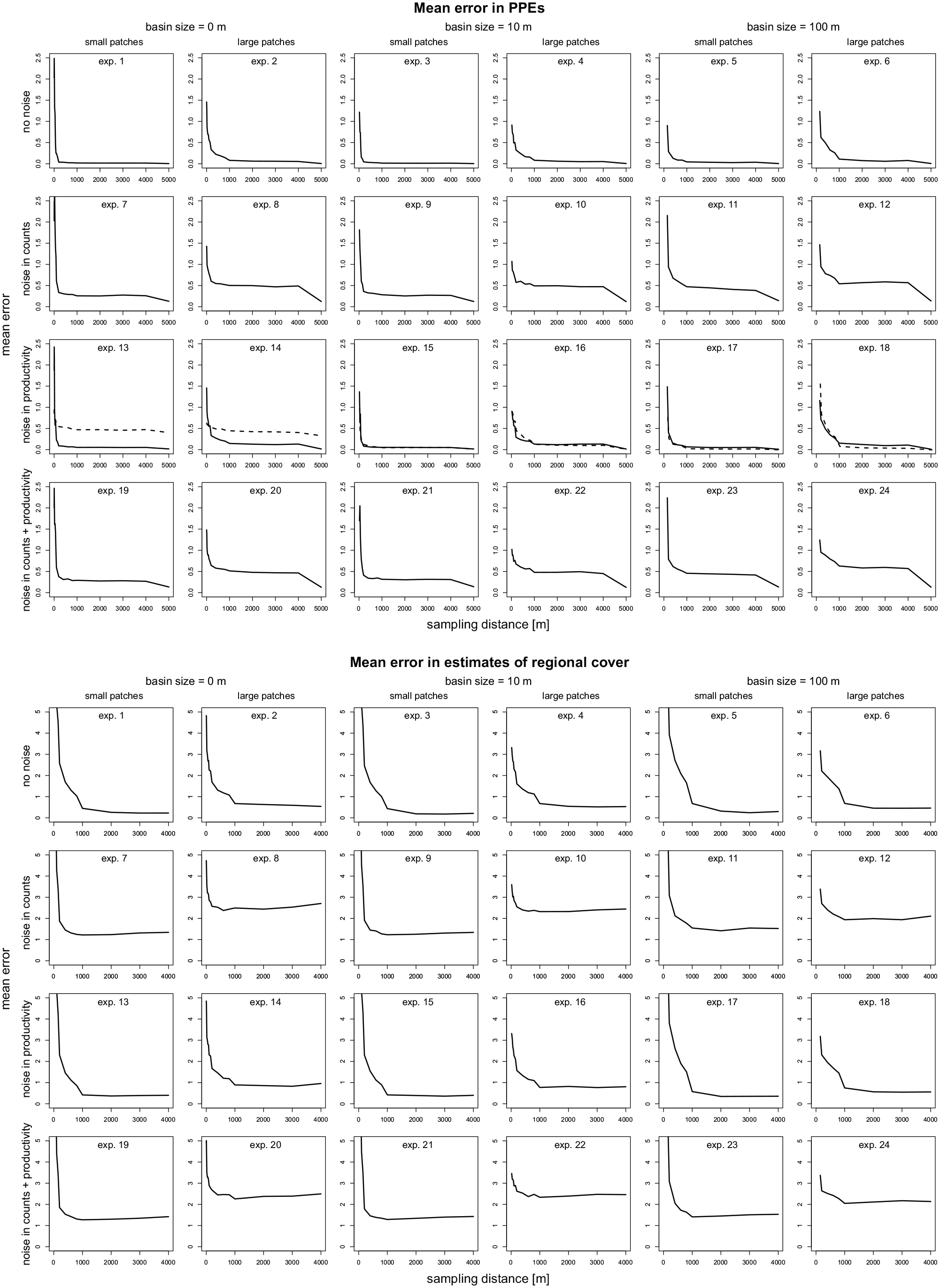
Accuracy of PPEs and regional cover in experiment 1–24 (Table 2) shown as rmse. For each experiment, rmse is calculated over all simulation with 10, 20, 30, 40, and 50 sites (=250 simulations). Experiment 13–18 were additionally run with the GPM dispersal model (dashed line).
Adding noise only to the pollen data (exp. 7–12) increases error in the resulting PPEs (Figure 3). After leveling off at ~1000 m sampling radius, the rmse remains at about 0.2–0.4 in the experiments with small patches (exp. 7, 9, 11) and at about 0.5–0.6 in the experiments with large patches (exp. 8, 10, 12; Figure 3). In experiments with noise in pollen productivity only (exp. 13–18) errors in the resulting PPEs are slightly higher than without noise. When applying the ERV with the GPM dispersal model, noise in pollen productivity results in higher errors in the experiments with a basin size of 0 m (exp. 13 and 14), but not in the experiments with larger basin size. With noise in pollen data and pollen productivity (exp. 19–24), errors in the PPEs are again clearly higher and about as high as with error in pollen counts alone.
Adding noise has similar effects on the resulting estimates of regional cover. Noise only in the pollen data (exp. 7–12) produces clearly increased errors in the estimated regional cover (Figure 3). Beyond ~1000 m sampling radius, the rmse of the regional cover estimates is about 1.5 with small (exp. 7, 9, 11, 13, 15, 17) and about 2.0–2.5 with large vegetation patches (exp. 8, 10, 12, 14, 16, 18). With noise in pollen productivity alone (exp. 13–18), errors in the regional cover estimates are only somewhat increased. With noise in pollen data and pollen productivity, errors in regional cover estimates are overall highest, that is, somewhat higher than with noise in pollen counts alone.
Effects of the number of sites
Errors in PPEs are highest for models run with only 10 sites and decrease when more sites are added (Figure 4). In most experiments the decrease is strongest in the step from 10 to 20 sites, particularly in the absence of noise (exp. 1–6, note the overall much lower error). The pattern is similar for errors in reconstructed regional cover (Figure 4).
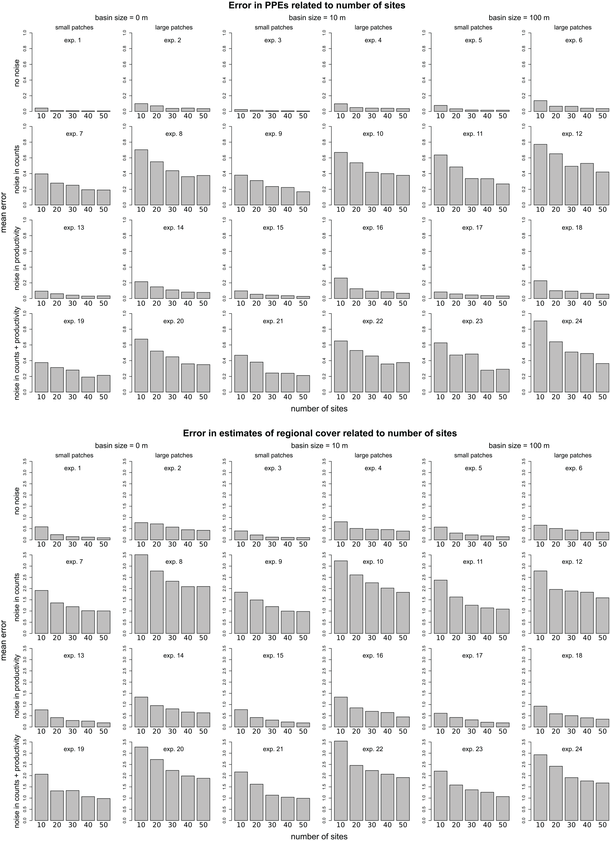
Rmse of PPEs and the estimated regional cover over number of sites in each experiment. The rmse is calculated as mean over 50 simulations, including only results for application with rings larger 1000 m radius.
Effects of basin size
Sampling vegetation in only short distance from the sampling point, as is often done in PPE-studies, may result in large errors in PPEs. If, but only if, vegetation cover from a large enough area is included in the model, changing basin size from 0 to 10 or 100 m has only little effect (Figures 3 and 5). The mean rmse of the PPEs calculated for rings >1000 m radius only, is 0.27 in experiments with 0 and 10 m basin size and slightly higher at 0.35 in experiments with 100 m basin size. The rmse in regional cover is 1.4 in experiments with 0 m basin size and 1.3 in experiments with 10 and 100 m basin size.
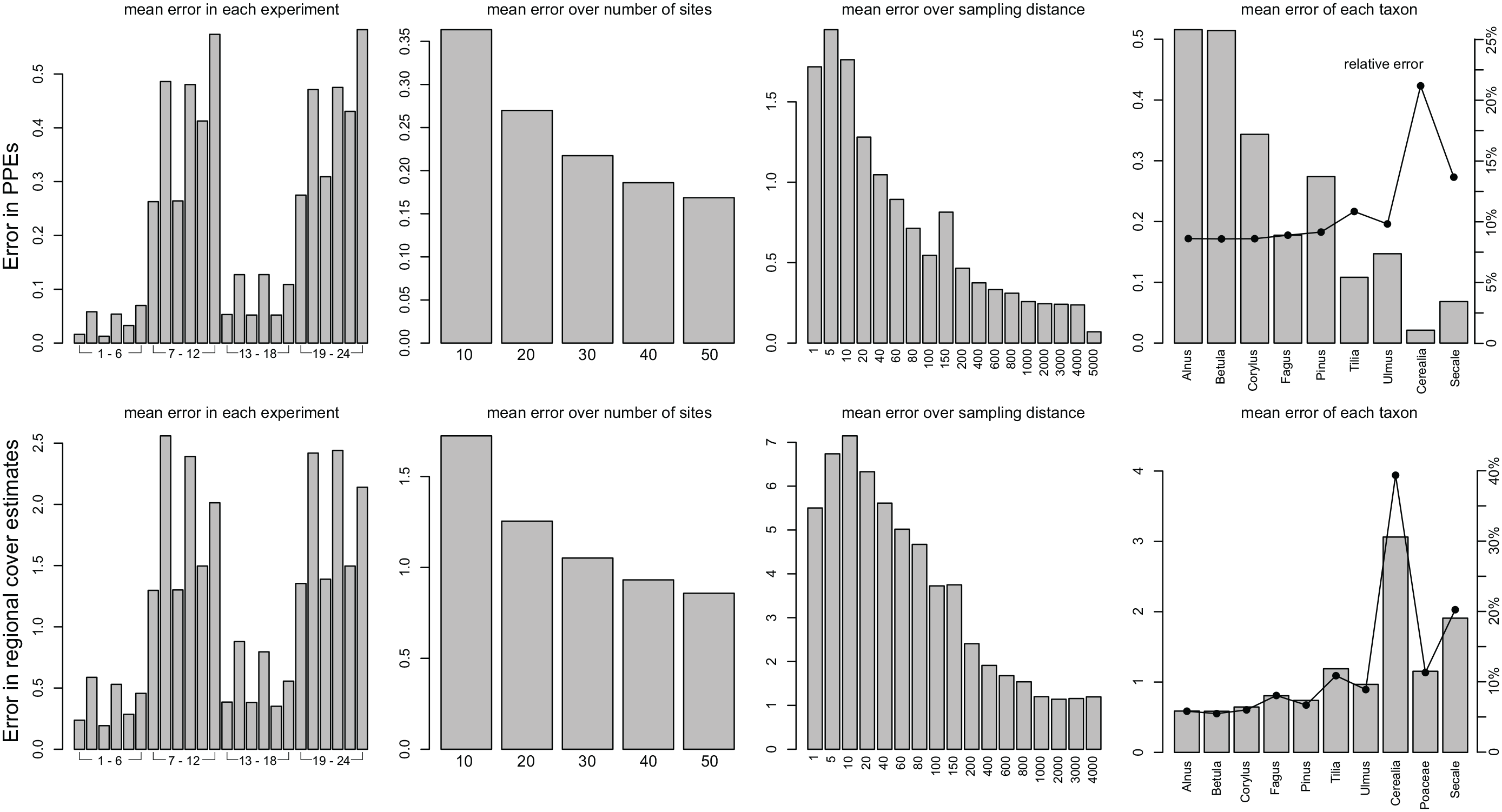
Mean error in PPEs and estimates of regional cover in each experiment, for each number of sites, for each sampling distance and for each taxon. Means over experiment, number of sites, and taxa were only calculated for sampling distances larger than 1000 m.
Effects of patch size
In general, for small vegetation patches, error in PPEs stabilizes at lower values and at smaller vegetation sampling radius than for large patches (Figures 3 and 5). This effect of patch size is most pronounced in the experiments with 0 and 10 m basin size. Here, PPE errors are twice as high with large (exp. 2, 4, 8, 10, 14, 16, 20, 22; Figure 5) than with small vegetation patches (exp. 1, 3, 7, 9, 13, 15, 19, 21). With 100 m basin size, PPE errors are only slightly higher with large (exp. 6, 12, 18) than with small patches (exp. 5, 11, 17, 23). Patch size has similar effects on errors in regional cover (Figure 5).
Errors in single taxa
Expressed as rmse, which means in absolute terms, errors in PPEs are closely correlated with the actual pollen productivity; errors are highest for Alnus and Betula and lowest for Cerealia and Secale (Figure 5). Relative errors (i.e. rmse divided by true pollen productivity) are instead highest for Cerealia and Secale, that is, the taxa with the lowest pollen productivity. Also the rmse in regional cover is highest for Cerealia and Secale (Figure 5). High errors in regional vegetation obviously relate to the high relative PPE errors in both taxa.
Goodness-of-fit (squared-chord-distance)
In our ERV implementation, PPEs are estimated by minimizing the squared-chord-distance between observed and modeled pollen percentage values. In theory, this distance should decrease with increasing vegetation sampling distance, that is, with each additional ring added in ERV analysis. In our experiments without noise (exp. 1–6; Figure 6) the squared-chord- distance indeed decreases with increasing sampling distance, approaching very small values of ~0.1. Hence, modeled and observed pollen values are nearly identical. The decrease is somewhat faster in the experiments with small vegetation patches (exp. 1, 3, 5), approaching a minimum already at ~1000 m sampling distance. With large vegetation patches (exp. 2, 4, 6), the squared-chord-distance remains overall slightly higher and continues to decrease until the final ring is added in the analysis.
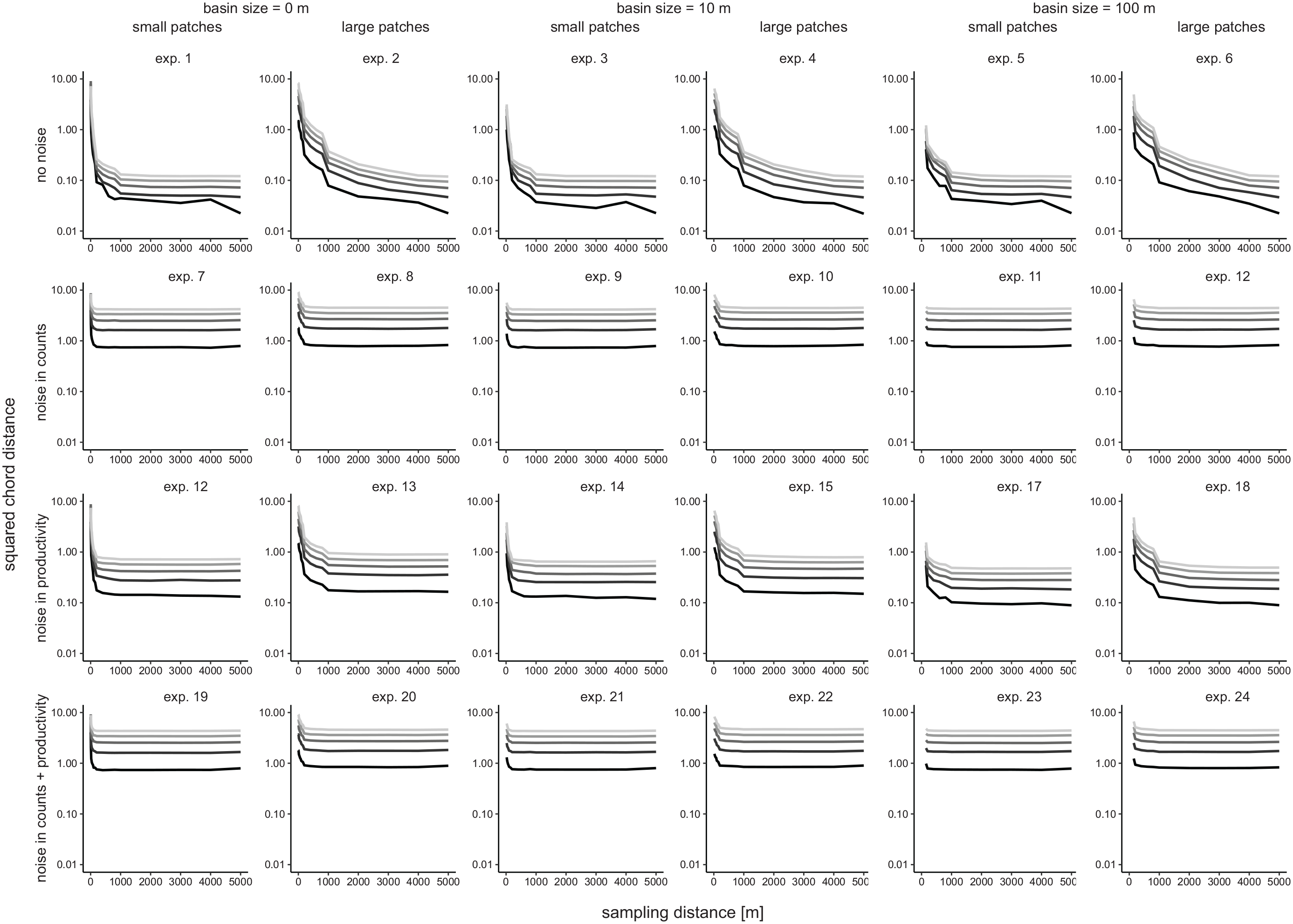
Mean squared chord distance between observed and modeled pollen values in each experiment in relation to the vegetation sampling distance. Gray tones indicate the number of sites, from 10 (light gray) to 50 (black). For each experiment and number of sites, 50 simulations were calculated.
In the more realistic experiments with noisy pollen data (exp. 7–24), the squared-chord-distance remains much higher (~0.5–5), reflecting that fitting modeled to observed pollen values is hampered by the noise in the pollen data. Moreover, the squared-chord-distance levels off already at small vegetation sampling distances of 200–1000 m (Figure 6). Hitherto, the sampling radius at which function scores (as analog to our squared-chord-distance) level off has been interpreted as the distance at which ERV analysis produces the most accurate PPEs. Yet, in our experiments, accuracy in the resulting PPEs increases at least until ~1000 m (Figures 3 and 6), that is, often beyond the distance at which the square-chord distance levels off. Similarly, accuracy in regional cover is highest with a vegetation sampling distance of at least 500–1000 m (Figures 3 and 6). So, with noise in the pollen data, the vegetation sampling distance at which squared-chord-distance levels off (i.e. the relevant source area of pollen sensu Sugita) is smaller than the sampling distance with the most accurate PPEs and estimates of regional cover.
Effects of dispersal model selection
Tests with the LSM-LSM combination (data sets created with LSM and ERV applied with LSM) and without noise produce precise and accurate results. The same applies to tests with the GPM-GPM combination (Figures 7 and 8). If the same dispersal model is used in creating the data sets and in ERV application, ERV produces accurate results.
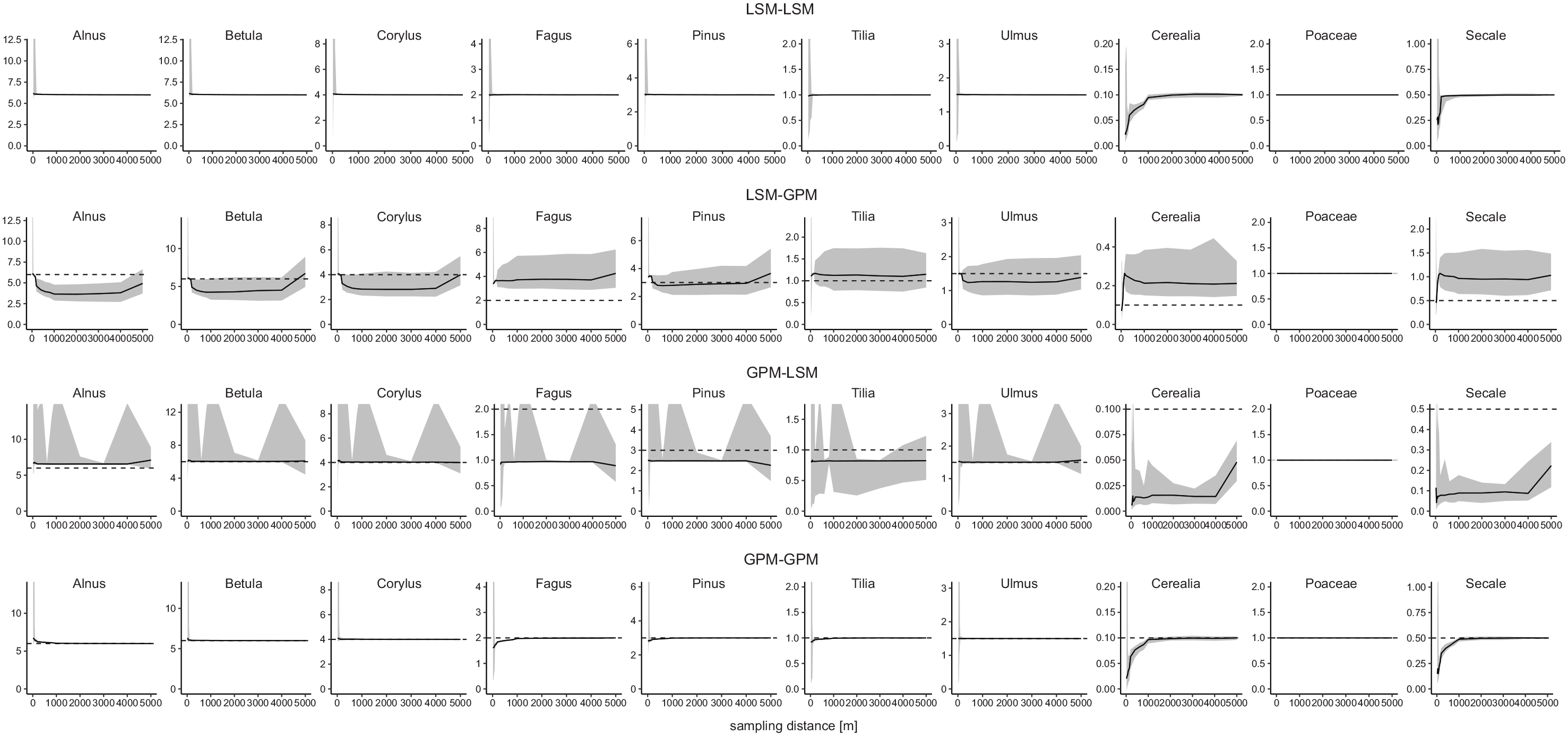
Median and confidence interval of PPEs calculated with different combinations of the LSM and GPM in the simulations. Calculations with 10 m basin size, 30 sites, no noise in the simulated data and 50 simulations. Dashed lines show true pollen productivitity.
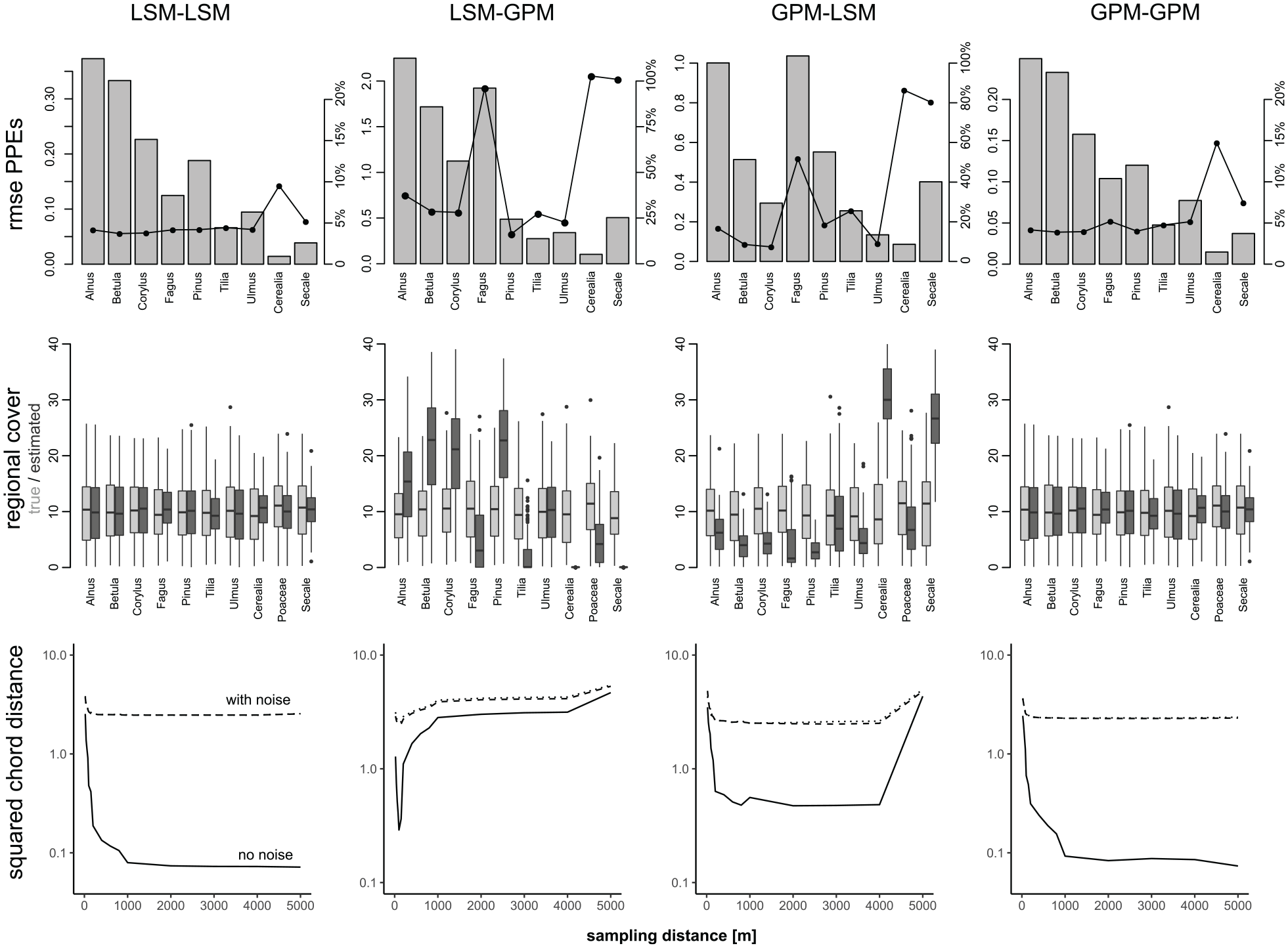
Error in PPEs, regional cover and optimized squared chord distances between simulated and modeled pollen values in experiments with different combinations of the LSM and GPM. Results show the mean of the experiments 3, 9, and 15 (10 m basin size, small patches, 30 sites, 50 simulations). Error in PPEs is shown as rmse (bars) and as rmse divided by true productivity (dots connected by lines). For regional cover, range of true values (light gray) and estimated valued (dark gray) shown. Squared chord distances are shown separately for experiment 3 (no noise – full line), 9 (noise in counts – dashed line), and 15 (noise in counts and productivity – dotted line).
In contrast, simulations with the LSM-GPM and GPM-LSM combinations show large errors in the resulting PPEs. With LSM-GPM, the PPE of Alnus (~3.5 instead of 6) is too low while the PPEs of Fagus (~4 instead of 2), Cerealia (~0.2 instead of 0.1), and Secale (~1 instead of 0.5) are too high (Figure 7). Deviations are smaller for the other taxa. Opposite errors occur with GPM-LSM: The PPE of Alnus (7 instead of 6) is too high while the PPEs of Fagus (~1 instead of 2), Cerealia (~0.02 instead of 0.1), and Secale (~0.1 instead of 0.5) are too low (Figure 7). Again, deviations are smaller for the other taxa. The errors relate to the fall speed of pollen, which has a much stronger effect on dispersal in the GPM than in the LSM (Theuerkauf et al., 2013, 2016). When the GPM is applied to a landscape where pollen dispersal is mimicked using the LSM, PPEs are too high for Cerealia, Fagus, and Secale (high fall speed) and too low for Alnus (low fall speed); when the LSM is used in a GPM landscape, errors are in the opposite direction (Figure 9).
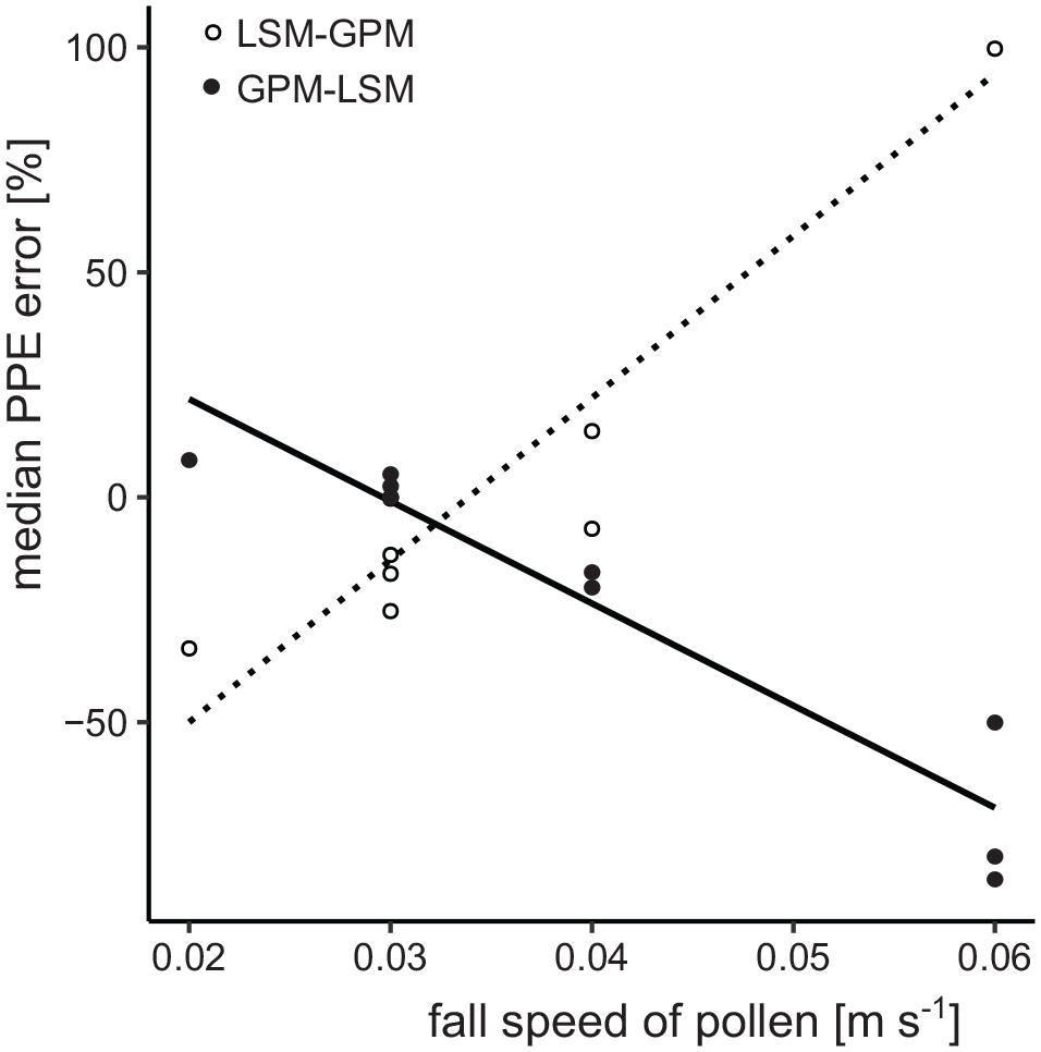
Relationship between median errors in PPEs and fall speed of pollen in experiments with a wrong dispersal model. Open dots: GPM used in ERV instead of the LSM, full dots: LSM used in ERV instead of the GPM.
The mixed dispersal model combinations not only add error in the median PPEs, but also reduce precision, meaning that there is large variation in the 50 simulations of each experiment (Figure 7). Similarly, errors in regional cover estimates are small with identical dispersal models in both steps (LSM-LSM and GPM-GPM) yet large, systematic errors appear when dispersal models are mixed, that is, when data sets are created with one model and ERV is applied with the other. With LSM-GPM, the estimated regional cover of Cerealia and Secale is always close to zero, independent of the true regional cover. Also for Fagus, Tilia, and Poaceae, the estimated regional cover is in most cases too low. Instead, for Betula, Corylus, and Pinus the estimated regional cover is too high. With GPM-LSM, errors are largely in the opposite direction; estimates of regional cover are clearly too high for Cerealia and Secale and mostly too low for the other taxa.
Finally, and as expected, with LSM-LSM and GPM-GPM, the difference between simulated and modeled pollen percentage values declines with increasing sampling radius and levels off at longer (no noise) or shorter distance (with noise, Figure 8). In contrast, with LSM-GPM, this difference reaches a minimum already at 20–100 m and then sharply increases again beyond that sampling radius. With GPM-LSM, this effect is less severe, but also here the difference reaches a minimum before it increases again when vegetation is sampled in larger rings.
Overall, we observe poor ERV performance when it is applied with a wrong dispersal model. The errors in PPEs are largest for Alnus, Fagus, Cerealia, and Secale: taxa with the lowest/highest fall speed of pollen that deviates most from the reference taxon. Moreover, results tend to differ substantially between single simulations. Apparently, errors differ in response to the specific vegetation pattern of each single simulation.
Discussion
Our simulations show good performance of the “ERVinR” function, which underlines the general suitability of the approach and proves the validity of our implementation. Application is straight-forward and can be automated, for example, for simulation studies like we present here. Beside the LSM, further dispersal options are available, and additional ones can be added. The programming code is available for validation and further development, for example, of the optimizer. In our tests, the “optim” function with the conjugate method (from base R) produced the most accurate results. Many further optimizers exist and future tests may identify even better methods. It may be worth testing whether different optimizers are suited for different types of data sets, for example, related to number of sites and taxa. Finally, our ERV implementation can be linked with other R functions to establish a faster workflow, for example, with GIS tools for the analysis of vegetation maps and with plotting tools to illustrate the results.
In ERV model 1 to 3, application is evaluated with scatterplots of adjusted vegetation proportion versus pollen proportion (ERV1), vegetation proportions versus adjusted pollen proportions (ERV2), and relative pollen loadings versus absolute vegetation (ERV3). In tests with simulated data, the plots for model 1 do not show the expected linear relationship, which is because the adjusted vegetation proportions account for the dispersal bias only. For models 2 and 3, the plots do show the expected linear relationships, although these are off the ideal and vary with the sampling radius of the vegetation cover (Figure 1). Our model 4 approach compares observed versus modeled pollen percentage values. Tests indeed show a linear 1:1 relationship in all cases (Figure 1).
Sugita (1994) suggested, that ERV application may be evaluated by comparing modeled with empiric regional pollen loading; calculated from regional vegetation composition and PPEs. As far as we know, such evaluation has not yet been applied in ERV studies. Our modified approach produces estimates of regional vegetation composition, which can readily be compared to observed regional composition as derived for example, from maps or forestry statistics. In many study areas, at least rough estimates of regional vegetation composition will be available. A prominent mismatch between estimated and real regional cover points at limitations of a given ERV application, for example, use of an unsuited dispersal model.
Limitations of the ERV approach
Aside from poor performance with small basins and limited vegetation mapping (<1000 m), two of the five parameters tested here – patch size and basin size – do not show a limiting effect on the ERV application in our experiments. As expected, accuracy of PPEs increases with the number of sites. High errors with only 10 sites suggest that ERV application can only provide a first approximation of PPEs if the number of sites is equal to the number of taxa. For robust results, the number of sites should higher than the number of taxa (cf. Li et al., 2018).
Two parameters, noise in the pollen data and dispersal model selection, obviously do play a critical role in ERV application. In our tests, noise in the pollen data added high relative errors in the PPEs of Cerealia and Secale − the taxa with lowest pollen productivity. As implemented, noise in the pollen data simulates the statistical uncertainty inherent to pollen counting – relative errors are highest for the lowest counts (Mosimann, 1965). Poor producers tend to be rare in pollen samples, even if abundant in the vegetation. Hence, ERV application is particularly sensitive for those low pollen producers, and other rare taxa in the pollen record. Counting errors may be reduced by higher counts. Still, also other sources of error in pollen data exist, for example errors related to pollen deposition and taphonomy or sampling and sample preparation. The size of these errors is difficult to estimate and likely differs much between studies.
Noise in pollen productivity has little effect in our simulations with the LSM, which is primarily because the local component of pollen deposition is rather small with the LSM. For Betula and a basin size of 0 m, the rings until 100 m radius contribute 25% of the total pollen deposition (Figure 2). Noise in pollen productivity has the largest effect in the smallest rings, and hence has overall little impact in our experiments. In contrast, simulations with the GPM show a high impact of noise in pollen productivity in experiments with a basin size of 0 m. The reason is that the GPM assumes a very high local component in pollen deposition. In the case of Betula and a basin size of 0 m, the GPM predicts that 70% of the total pollen deposition arrives from within 100 m distance, 47% alone from the innermost ring (Figure 2). Hence, noise in pollen productivity has a much larger effect. As we discuss in more detail below, predictions of the GPM are obviously unrealistic. It particularly under-estimates dispersal distances of larger and heavier pollen grains, likely because the model assumes pollen emission at ground-level (Figure 10). Hence, the model apparently overestimates the local component of pollen deposition. Nonetheless, even with the GPM noise in the pollen productivity only has prominent effects with a basin size of 0 m. Hence, plant-to-plant differences in pollen productivity appear to be only a minor disturbance for ERV application with larger basins.
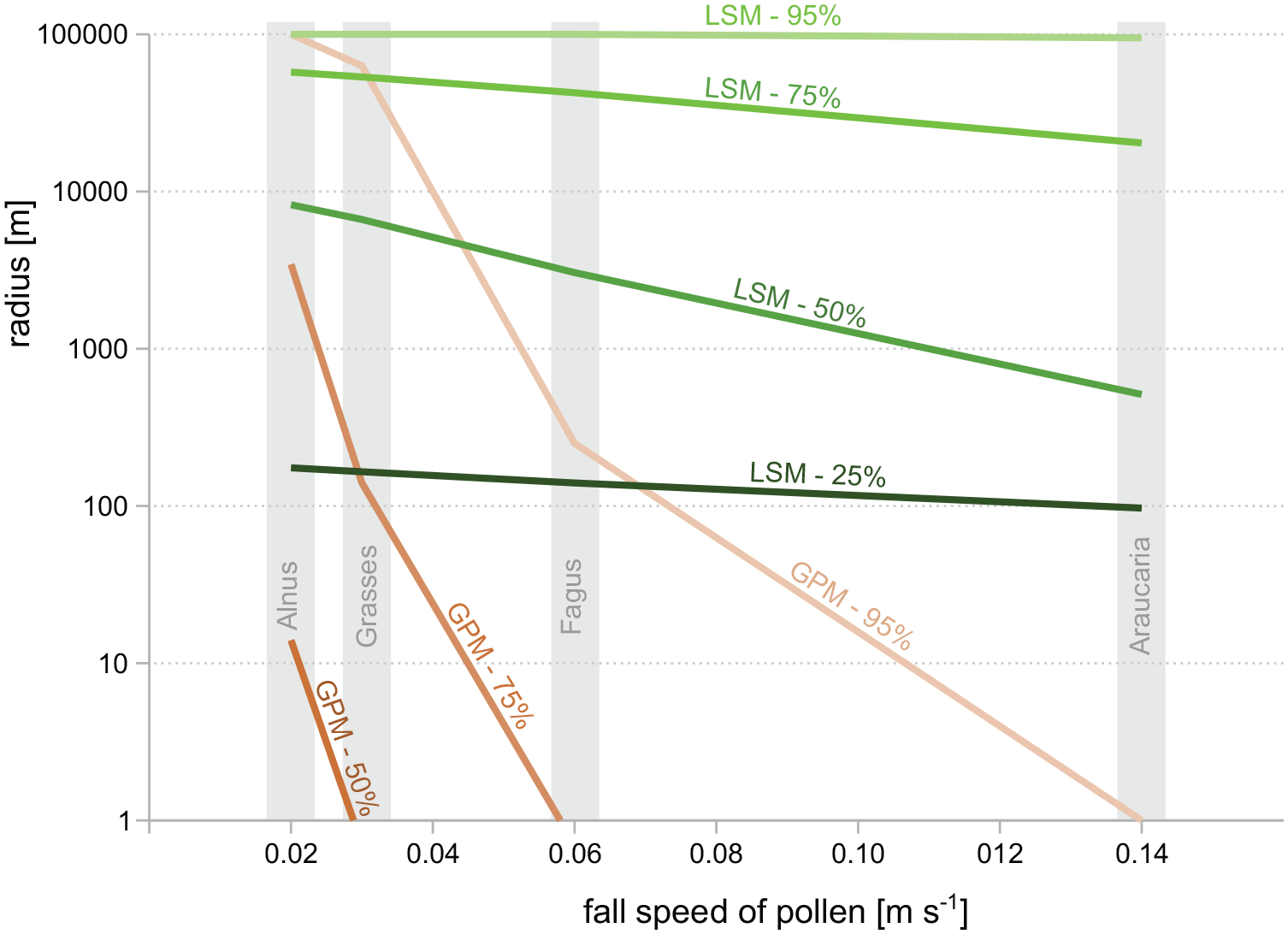
Source area of pollen calculated with the LSM of Kuparinen et al. (2007) and the GPM following Prentice (1985). Source areas calculated for falls speeds from 0.02 to 0.14 m s−1 and for a sample taken inside vegetation, that is, with basin size = 0 m. Source area shown as the area from which 25% (only LSM), 50%, 75%, and 95% of the total pollen deposition arrives.
In several tree taxa, in Central Europe for example Fagus sylvatica and Picea abies, pollen productivity differs strongly from year-to-year (Pidek et al., 2010). In the case of Fagus sylvatica, years with peak pollen production occur in variable intervals from 2 to 10 years (Theuerkauf et al., 2019). With such taxa present in the vegetation, ERV application requires pollen samples that integrate pollen deposition over sufficiently long periods, for example, lake surface sediment samples or a series of annual pollen trap data. Moss pollster samples, which often integrate 1 or several years only, may be unsuited to accurately represent pollen productivity of such taxa.
Highest errors in in our simulations are related to dispersal model selection. By using different pollen dispersal models in (i) creating the simulated pollen datasets and (ii) the ERV application we simulate the real-world problem that no pollen dispersal model is perfect, that is, that dispersal patterns described by dispersal models will be more or less different from the true dispersal patterns in a given study region. Dispersal patterns predicted by the LSM and GPM differ largely. First, the GPM overall predicts much shorter dispersal distances and hence source areas. Distance weighting with this model gives much more weight to vegetation near a sample site than the LSM (Theuerkauf et al., 2013). Moreover, fall speed of pollen has a much larger impact in the GPM than in the LSM so that the GPM predicts much shorter dispersal and hence smaller source areas for taxa with large pollen with high fall speed. With the GPM, 95% of the pollen of Araucaria would arrive from <1 m distance, from ~250 m for Fagus and from >100 km for Alnus (Figure 10). These large differences in source area are obviously unrealistic. They imply that distance weighting with the GPM gives much less weight to Fagus than to Alnus, for example. In the LSM, the impact of fall speed is small and even negligible for fall speeds smaller than 0.04 m s−1 (Kuparinen et al., 2007). Hence, distance weighting gives only slightly less weight to Fagus than to Alnus. So, when ERV is applied with the GPM instead of the LSM, we arrive at too high PPEs for Fagus as a taxon with higher fall speed. The relationship is simple: pollen deposition at a site is related to distance weighted abundance multiplied by pollen productivity (equation (2)); if pollen deposition is the same, then lower distance weighted plant abundances imply higher PPEs. The opposite applies for taxa with low fall speed like Alnus.
In the experiments where ERV is applied with a different dispersal model than the one used to simulate the pollen datasets, we observed highly variable results in each of the 50 model runs. These variations are likely due to differences in vegetation composition in the single model runs. Errors in PPEs are higher in simulations with a high cover of taxa with high/low fall speed. This effect may in part explain inconsistencies in real-world ERV applications from one and the same region, but with different overall vegetation composition. The conclusion would then be, that the dispersal model used in these studies did not approach reality.
Is there a suitable dispersal model?
Most ERV studies so far have used the so called Prentice model, which is a Gaussian plume model based on Sutton’s equations of a ground-level particle source (Prentice, 1985). This class of models has well known conceptual limitations with respect to pollen dispersal (Kuparinen et al., 2007; Sofiev et al., 2013). Particularly the strong impact of fall speed is unrealistic, as discussed above. Moreover, the overly short dispersal distances in heavier pollen types are obviously due to the fact that the Prentice model assumes dispersal from ground level (Jackson and Lyford, 1999).
In regional scale studies, with pollen samples from lakes, the LSM of Kuparinen et al. (2007) has shown to be a more suitable dispersal model than the GPM (Theuerkauf et al., 2013). ERV studies usually collect pollen samples from moss polsters or pollen traps inside closed vegetation. Here, pollen deposition is dominated by pollen traveling only short distances (~0–100 m), and the pollen signal is dominated by (extra)local pollen deposition (Janssen, 1973). The dominance of local pollen deposition comes with two complications.
First, the (extra)local part of the dispersal curve is its steepest part, implying that pollen deposition from a plant in 1 m distance from a site is much higher than pollen deposition from similar plants in 5 or 20 m distance. Proper distance weighting therefore requires a dispersal model that describes the steep local part of the dispersal curve extremely well. Moreover, pollen deposition is strongly influenced by the closest pollen sources, which in some cases means by a few plants only. The health, age, and competitive position of these plants in the immediate vicinity drive pollen deposition to a large extent. The steep part of the dispersal curve is less relevant for regional scale studies.
Secondly, dispersal on (extra)local scales is further complicated by several factors, such as differential release height and vegetation density. Pollen emitted from a tall grass in a treeless vegetation or from a single tree in semi-open vegetation will be dispersed much farther than pollen released near the ground. In tall and dense vegetation, wind speeds are lower and more pollen is filtered out than in short and open vegetation. Forest edges produce eddies, that influence dispersal on (extra)local scales. The existence of such disturbing effects is long known, but it remains difficult to quantify them (Jackson and Lyford, 1999; Tauber, 1965). If dispersal is mostly driven by these disturbances rather than by regular airflow patterns, even advanced dispersal models like the Kuparinen LSM will be unsuited if they are not modified to address such disturbing factors. LSMs may be adjusted to spatial patterns in vegetation to include, for example, differential release height and vegetation density. Still, efforts to measure these parameters in the field and implement them in the model will be high.
Using the LSM to create pollen data and then the GPM to estimate PPEs, and vice versa, the squared chord distance between between simulated and modeled pollen (similar to likelihood function scores in previous ERV applications) does not show the expected asymptotic decline but increases again with larger rings added. Apparently, when observed in a PPE study, such pattern indicates that the dispersal model used does not match true pollen dispersal.
Considering the key role of an appropriate dispersal model in ERV studies, and the potentially large disturbing effects on the (extra)local scale, ERV application with local scale pollen data appears particularly challenging, if not impossible. The known errors and limitations of the Prentice GPM clearly make future applications of this model questionable. The suitability of the Kuparinen LSM for local-scale ERV studies needs further evaluation, for example by re-analysis of existing ERV studies (cf. Marquer et al., 2020; Theuerkauf and Couwenberg, 2020).
Vegetation sampling area
A key question in ERV application is to find the minimum vegetation sampling radius needed for accurate results. The common approach is to use the radius at which “likelihood function scores” approach an asymptote (our approach in analog uses the squared chord distance between modeled and observed pollen percentage values). This distance is then named the “relevant source area of pollen” (RSAP) in Sugita (1994). The RSAP is supposed to be primarily a measure of vegetation patch size (Bunting et al., 2004; Sugita, 1994). Our simulations without noise indeed show a larger RSAP with larger patches. However, in the more realistic simulations with noise, squared chord distances reach the asymptote at a smaller vegetation sampling distance, although with a much lower closeness of fit (Figure 6). The optimization simply cannot fit the modeled pollen values as closely to the observed pollen values when the latter are noisy. The RSAP is now similar for small and large patches. While noise in the pollen data reduces the RSAP, it does not change the vegetation sampling distance at which the most accurate PPEs are calculated, which is still 1000 m or beyond (Figure 3). Hence, with noise in the pollen data, the RSAP tends to underestimate the best sampling distance. Further experiments are needed to explore whether and how this effect changes with the degree of noise in the pollen data.
Site selection for ERV analysis
The ERV model is designed to estimate PPEs with pollen samples that include (extra)local pollen deposition, that is, pollen samples from pollen traps, moss polsters or small lakes. For robust results, calibration should cover long gradients in plant abundances and pollen deposition. Local vegetation composition and thus pollen deposition should differ substantially between sample sites. At the same time, the ERV model requires that regional pollen deposition, that is, regional vegetation composition, is uniform at all sites. Hence, the ERV model is best suited for landscapes with a fine-grained vegetation mosaic that provides sufficient local-scale variation among sample sites, yet overall uniform vegetation composition that delivers uniform regional pollen deposition. In landscapes with either large vegetation patterns or vegetation gradients ERV application is problematic. Here, uniform regional pollen deposition is only warranted if the sample sites are located close to each other. In this case differences in local vegetation composition and hence pollen deposition may be too small for robust ERV application, however. We discuss alternative approaches to produce PPEs in such landscapes in the following section.
Our results indicate that ERV application is probably most challenging with pollen samples from the smallest “basins,” that is, from moss polsters or pollen traps placed inside vegetation. Pollen deposition in such samples may be most biased by particular pollen dispersal patterns on the local-scale and by variable pollen productivity. Regional-scale pollen dispersal, which determines pollen deposition in large lakes, is mostly governed by the general atmospheric conditions prevailing in a region. These regional scale dispersal patterns can obviously well be implemented in state-of-the-art pollen dispersal models (Theuerkauf et al., 2013). Pollen dispersal and deposition on the local-scale is more complex because it is affected by additional factors, particularly by the vegetation structure of the sample site. For example, pollen released from a tall tree will likely be dispersed farther than pollen from a tall herb. Also, herb pollen released in a sheltered open patch in a forest will likely be dispersed less far than herb pollen released in more exposed vegetation. Single trees and forest edges produce eddies and channel airflows, which influence pollen dispersal. Finally, dispersal inside vegetation, within a forest, is determined by vegetation density. All these factors are particularly relevant in semi-open landscapes, where vegetation structure and hence pollen dispersal patterns may differ substantially between sample sites. The Prentice dispersal model, which is hitherto commonly used in ERV analyses, does not account for such effects. The LSM we used in the present study is adjusted to pollen dispersal in and above a pine forest (Kuparinen et al., 2007). It may be adjusted to other vegetation types as well, such as open vegetation. It is questionable, however, whether the model can be adjusted, with reasonable efforts, to the small scale mix of different vegetation types in semi-open settings, with complex airflow patterns and different release heights of pollen.
A second limitation for ERV application with pollen samples from pollen trap or moss polsters is variable pollen productivity of individual plants, caused by different fitness, age, or site conditions etc. Our results suggest that varying pollen productivity can be a disturbing factor in ERV application with the smallest sites. The effects were much higher with the GPM than with the LSM because the local component of pollen deposition is large with the GPM yet small with the LSM. As discussed above, the local component is likely overestimated with the GPM because the model assumes release at ground level. The LSM my instead underestimated local pollen deposition, for two reasons. First, the LSM we used is adjusted to pollen dispersal in a pine forest with a mean release height of pollen at about 12 m. In (semi) open vegetation, (most) pollen is released at lower heights, likely resulting in lower dispersal distances and hence a higher local component of pollen deposition. Secondly, all pollen dispersal models only account for pollen transported by air in dry conditions. In reality, some pollen may not enter the airflow but is washed-down by rainfall near the source plant. Also, flowers may fall down before all pollen is released, potentially adding pollen to local deposition in pollen traps and moss polsters. A higher local component implies that the disturbing effects due to small-scale variations in pollen production would be higher than in our experiments with the LSM.
We cannot evaluate how much the mentioned factors indeed hamper ERV application with pollen samples from pollen traps and moss polsters. A recent ERV study from the Araucaria forest-grassland mosaic in souther Brazil suggests that the complications due to differential release height of pollen are indeed relevant (Piraquive Bermúdez et al., 2021). Such semi-open settings likely require a better understanding of the disturbing factors to arrive at robust PPEs. On the other hand, the results of Andersen (1970) suggest that data from pollen traps inside forests do allow robust calibration of the pollen-vegetation relationship. In this case, however, disturbing factors may have been reduced because all samples are from the same vegetation type, that is, old growth forest, and only includes tree taxa, hence avoiding the problems due to differential release height.
The above complications can likely be reduced with pollen samples from small openings in the (pollen producing) vegetation, for example, small lakes. Peatlands may be suited as well, particularly if peatland vegetation is open and does not produce the pollen types of interest in the ERV study.
Where suitable lakes and peatlands are missing, pollen traps installed in open spots with no pollen producing vegetation may provide an alternative. As mentioned, current pollen dispersal models do not account for the particular challenges that are relevant on local scales, such as differential release height of pollen. Further research is needed to explore the impact of for example, release height in a first step. If that impact is indeed high, models suitable to account for this and other disturbing factors would be needed.
Alternatives to the ERV model
A main benefit of the ERV approach is that it requires limited vegetation mapping. As mentioned above, the assumption of uniform background pollen deposition limits ERV application to landscapes with a fine grained vegetation mosaic and overall uniform vegetation composition. ERV is not suited for landscapes with large vegetation patches (>several km grain size) or with vegetation gradients. In such landscapes, PPEs may instead be produced with approaches that do not rely on the assumption of uniform regional pollen deposition, like the optimization approaches of Theuerkauf et al. (2013) or Fang et al. (2019). These approaches best work with pollen data from lakes and require mapped vegetation data from much larger areas, for example, from a 30 km radius in Theuerkauf et al. (2013). Producing such data is increasingly feasible due to the increasing availability of forest and land use data bases as well as improved vegetation classification from remote-sensing data (e.g. Preidl et al., 2020).
Another approach is to pool local scale pollen samples and estimate PPEs with the inverse REVEALS model (Kuneš et al., 2019). Whether and in which settings the approach is suited to avoid difficulties of local scale pollen samples may need further evaluation.
In addition, pollen productivity may be estimated directly by estimating the number of pollen per flower and the number of flowers per plant or area (e.g. Pohl, 1937). This approach is more labor-intensive and is hence less suited to produce comprehensive PPE data sets for a given study region. Still, the approach has several benefits. For example, it produces pollen productivity numbers in absolute terms, it enables to study pollen productivity on the species level, and – much better than pollen sample based approaches – it allows to study pollen productivity on a single plant or stand scale. In conclusion, the approach is suited to explore the influence of, for example, climate, site conditions or tree age on pollen productivity of single taxa. The influence of age may be particular important to validate PPEs produced with ERV in landscapes with managed forests. Median tree ages in managed forests are usually much lower than in natural forests. Considering that younger trees likely produce less pollen, PPEs estimated in the modern cultural landscape may underestimate pollen productivity for periods in which natural forest cover was dominant, leading to skewed reconstructions. Directly estimated pollen productivities may be one way to identify and eventually correct for such effects.
Finally, pollen productivity may be estimated from fossil pollen records with the ROPES approach (Theuerkauf and Couwenberg, 2018), which requires well dated, high resolution pollen records with substantial variation present in each pollen type. Besides eliminating time-consuming vegetation mapping, the main advantage of ROPES is that it allows to estimate PPEs for distinct periods of the past, that is, for periods prior to intense land-management. ROPES avoids bias in modern-day PPEs that is related to present-day land management, the changing climate or elevated atmospheric CO2 concentrations. All three factors have significantly altered pollen production in plants over the past decades (e.g. Rogers et al., 2006; Theuerkauf et al., 2015; Ziska et al., 2019).
Conclusions
The “ERVinR” function enables application of the ERV model in the R environment for statistical computing. The function allows for flexible parameter selection and full control over the underlying assumptions and calculations, which is open to further development. “ERVinR” allows for repeated calculations (e.g. 100 times) and leave-one-out approaches to evaluate robustness of ERV applications. Moreover, it provides estimates of regional vegetation composition, which help to evaluate the success of the ERV application. The function allows for setting up simulation studies, as presented in this paper, for example, to further explore critical parameters of the model.
With help of the function, we identified noise in the pollen counts and dispersal model selection as two critical parameters in ERV applications. Count errors in pollen data reduce accuracy of the calculated PPEs particularly for the taxa rare in the pollen record, which are usually taxa that produce very little pollen. High count sums will reduce this type of error. We propose to use simulations to estimate the effects. Noise in the pollen counts also tends to reduce the distance at which squared chord distance (as equivalent to function scores) levels off, that is, the relevant source area of pollen (RSAP). Hence, the calculated RSAP may be smaller than the sampling distance for which the best PPEs are actually calculated. Also here, simulations may help to better estimate the best sampling radius for a given data set. Noise in pollen productivity had minor effects in our experiments with the LSM, yet it may be an important factor if local pollen deposition is higher than projected by the LSM.
Successful ERV application depends on a suitable dispersal model. We propose using state-of-the-art Lagrangian-Stochastic models. The disqover package provides an LSM option adjusted to pollen dispersal in a forest under the atmospheric conditions in northern central Europe. In other regions, models adjusted to the particular conditions should be used. We suggest consulting local experts for actual model selection and parameter settings in other study regions.
Currently, no available dispersal model is adjusted to the more complex dispersal patterns on local scale, which are additionally determined by release height and vegetation structure, for example, particularly in semi-open vegetation. Here, all current dispersal models are likely deficient for ERV application with pollen data from pollen traps and moss polsters inside vegetation, where the local-scale dispersal processes are most relevant. To reduce the associated disturbing effects in ERV application, we propose using surface pollen data from small natural or artificial openings in the vegetation. However, for the time being and to our judgment, the best way to achieve valid PPEs for application in paleo-ecological studies is with surface pollen data sets from large sites with prevailing regional pollen deposition, which can well be handled with existing dispersal models. Working with such sites requires alternative approaches, however.
Footnotes
Acknowledgements
We thank Shinya Sugita for providing the ERV.Analysis.v2.5.3 program and are grateful to two anonymous reviewers for helpful comments. This study was undertaken as part of LandCover6k, a working group of the Past Global Changes (PAGES) project, which in turn received support from the Swiss Academy of Sciences and the Chinese Academy of Sciences.
Funding
The author(s) disclosed receipt of the following financial support for the research, authorship, and/or publication of this article: This study is a contribution to BaltRap: The Baltic Sea and its southern Lowlands: proxy – environment interactions in times of Rapid change (SAW-2017-IOW2). The work of JC was funded by the European Social Fund (ESF) and the Ministry of Education, Science and Culture of Mecklenburg-Western Pomerania (project WETSCAPES, ESF/14-BM-A55-0030/16).