Sage Journals: Discover world-class research

Abstract

Relative sea-level (RSL) records from far-field regions distal from ice sheets remain poorly understood, particularly in the early Holocene. Here, we extended the Holocene RSL data from Singapore by producing early Holocene sea-level index points (SLIPs) and limiting dates from a new ~40 m sediment core. We merged new and published RSL data to construct a standardized Singapore RSL database consisting of 88 SLIPs and limiting data. In the early Holocene, RSL rose rapidly from −21.0 to −0.7 m from ~9500 to 7000 cal. yrs. BP. Thereafter, the rate of RSL rise decelerated, reaching a mid-Holocene highstand of 4.0 ± 4.5 m at 5100 cal. yrs. BP, before falling to its present level. There is no evidence of any inflections in RSL when the full uncertainty of SLIPs is considered. When combined with other standardized data from the Malay-Thai Peninsula, our results also show substantial misfits between regional RSL reconstructions and glacial isostatic adjustment (GIA) model predictions in the rate of early Holocene RSL rise, the timing of the mid-Holocene highstand and the nature of late-Holocene RSL fall towards the present. It is presently unknown whether these misfits are caused by regional processes, such as subsidence of the continental shelf, or inaccurate parameters used in the GIA model.

Keywords

Holocene sea level basal peat sediment compaction Sunda Shelf Glacial Isostatic Adjustment (GIA)

Introduction

The Holocene epoch was marked by substantial temporal and spatial variations in relative sea level (RSL) (e.g. Kidson, 1982; Smith et al., 2011). Temporally rapid RSL rise during the early Holocene (11,700–7000 cal. yrs. BP) provides a potential analogue for understanding future sea-level rise (Fleming et al., 1998; Törnqvist and Hijma, 2012). During the early Holocene, global mean sea-level (GMSL) rose by up to 60 m (Lambeck et al., 2014; Smith et al., 2011) due to meltwater mainly derived from the final deglaciation of the Laurentide and Fennoscandian ice sheets (Stroeven et al., 2016; Ullman et al., 2016). The early Holocene is also characterized by a possible ‘stepped’ rise in GMSL (e.g. Hori and Saito, 2007; Liu et al., 2004) from meltwater events (e.g. Törnqvist and Hijma, 2012).

Spatially, Holocene RSL differs from GMSL mainly due to glacial isostatic adjustment (GIA), which is the dynamic response of the lithosphere and mantle to ice-water loading and unloading events during a glacial cycle (e.g. Mitrovica et al., 2001; Peltier, 1999; Peltier and Andrews, 1976). Larger GIA signals are found in regions that were beneath (near-field) or at the margins (intermediate-field) of the Laurentide and Fennoscandian ice sheets where loading/unloading of ice produced deformation of the solid Earth (e.g. Clark et al., 1978; Milne, 2015; Peltier, 2004). The reverse is true for regions distal from the northern hemisphere ice sheets (far-field), where the surface deformation component of the signal reduces in magnitude and so the eustatic (or meltwater) signal becomes dominant (Fleming et al., 1998).

In contrast to near- or intermediate-field regions, sea-level reconstructions from far-field regions, particularly during the early Holocene, are poorly constrained (e.g. Horton et al., 2005). In this study, we reconstruct Holocene RSL data from Singapore, which lies at the tip of Peninsular Malaysia (Figure 1a) in the core of the tectonically stable Sundaland (Tjia, 1996). There have been several notable attempts to produce a far-field Holocene RSL record for the Singaporean region (e.g. Bird et al., 2007, 2010; Hesp et al., 1998). However, the criteria necessary to produce accurate sea-level index points (SLIP) in Singapore (Bird et al., 2007, 2010) have infrequently been met (Khan et al., 2019). A sea-level index point (SLIP) estimates the position of relative sea level (RSL) at a particular point in space and time (Shennan and Horton, 2002). SLIPs must contain information regarding the relationship of the sample to a contemporary tidal level (termed the indicative meaning) (van de Plassche, 1986). Since RSL are seldom reconstructed from a single type of sea-level indicator, each indicator is related to its own contemporary tide level (reference water level) such as mean tide level (MTL), mean high water spring tides (MHWST) or highest astronomical tide (HAT) (Engelhart et al., 2011). Developing an accurate SLIPs from radiocarbon ages requires evaluation of all available information about radiocarbon samples and their stratigraphic or geomorphic context. A source of error in RSL studies stems from the calibration of radiocarbon dated samples to calendar years (e.g. Törnqvist et al., 2015). If ages are calibrated, different calibration programs are often used, and they produce slightly different results. Larger uncertainties are introduced by the application of corrections for the marine reservoir effect (e.g. Alves et al., 2019; Hua et al., 2015).

Figure 1.

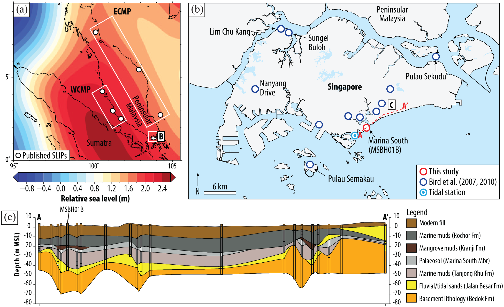
(a) Glacial isostatic adjustment (GIA) relative sea-level (RSL) predictions ICE-6G_C (Peltier et al., 2015) in Southeast Asia at 5000 cal. years. BP. White rectangles show the locations of three study regions, namely the west coast of the Malay-Thai Peninsula (WCMP), Singapore and the east coast of the Malay-Thai Peninsula (ECMP). Locations of individual study sites are denoted by white dots. (b) Map of Singapore showing the locations of sediment core MSBH01B (this study) and study sites of published relative sea-level reconstructions (Bird et al., 2007, 2010), shown as red and blue circles, respectively. The location of the Tanjong Pagar tidal station is shown as a light blue dotted circle. (c) Cross-section of Transect A – A′ showing the local stratigraphic succession and location of MSBH01B. The vertical exaggeration of the cross-section is set at 25 times (modified from Chua et al., 2020).

Here, we produced new SLIPs from a ~40 m continuous sediment core (MSBH01B) obtained from the southern tip of mainland Singapore (Figure 1b) to extend the RSL record to the early Holocene. In addition, we re-evaluated published data from Bird et al. (2007, 2010) following the methodology of HOLocene SEA-level variability (HOLSEA) working group (Khan et al., 2019). We assessed the existence of an inflection in the rates of RSL rise centred at ~7600 cal. yrs. BP previously suggested by Bird et al. (2010). We compared the revised RSL reconstructions for the Singapore region with a subset of the regional Southeast Asia, database (Mann et al., 2019) and the latest iteration of GIA models (Li and Wu, 2019; Peltier et al., 2015) to better understand the driving mechanisms of temporal and spatial variability in Holocene RSL data.

Study area

Singapore is a small island (~725 km²) situated at the tip of Peninsular Malaysia (Figure 1a), which is a tectonically stable extension of Southeast Asia’s continental Sunda Shelf (Tjia, 1996) that was exposed during the glacial periods of the last two million years (Hanebuth et al., 2000, 2009). Singapore’s basement geology comprises late Palaeozoic and Mesozoic sedimentary rocks and intrusive igneous units, which are overlain by weathered shales and sandstones possibly of middle Triassic to lower Cretaceous age (Dodd et al., 2019). The Quaternary deposits, mostly found in southern Singapore, consist of fluvial sands and clays of Pleistocene age (Gupta et al., 1987). These fluvial deposits are succeeded by littoral/fluvial sands, organic peats and marine muds deposited possibly during interglacials of the late Pleistocene (~125 ka BP). The desiccated late Pleistocene marine muds (Marina South Member) acts as a distinct stratigraphic marker (Figure 1c) for the Holocene marine transgression (Chua et al., 2020).

Singapore is meso-tidal, with a mean tidal range of 2.4 m during spring tides and 1 m during neap tides (Wong, 1992). These tide levels are measured to a fixed Chart Datum, established to be 1.65 m below Singapore Height Datum (SHD) Tanjong Pagar tidal station (1°15.7′ N, 103° 51.1′E).

The coring site, Marina South (Figure 1b), is a reclaimed area on the southern coast of Singapore, which was previously a sandy estuarine mudflat environment fed by three converging tributaries (Chua et al., 2016). The data of Bird et al. (2007, 2010), which incorporates the RSL data of Hesp et al. (1998), was obtained from 12 locations in Singapore: seven locations from south and southeast Singapore; two from the mangrove-dominated northwest coastline at Sungei Buloh and Lim Chu Kang; one from a tidal creek at Nanyang Drive; and two from the offshore islands of Pulau Semakau and Pulau Sekudu (Figure 1b).

Methodology

Collection of Holocene sediment core

We obtained a continuous 38.5 m long sediment core (MSBH01B) from 1.27266° N, 103.8653°E at Marina South (Figures 1b and c) using a rotary drilling machine coupled with a hydraulic piston and Selby thin-walled core tubes. The elevation of core MSBH01B was measured using a Leica System 2000 TCA1800 total station, which was then related to SHD. We converted all elevations from SHD to mean sea level (MSL) using the nearby tidal data from Tanjong Pagar tidal station (Figure 1b).

We focused on the Holocene section of the core (+4.1 m to −20.0 m MSL) (Figure 2). The top ~12 m of sediment was modern fill material and removed. Recovery of the remaining sediment was at least 90% with little slump loss or compaction during coring. Core material was removed by a motorized horizontal core extruder and housed in split PVC pipes, wrapped in plastic film, and stored at ~4^oC to prevent sample deterioration.

Figure 2.

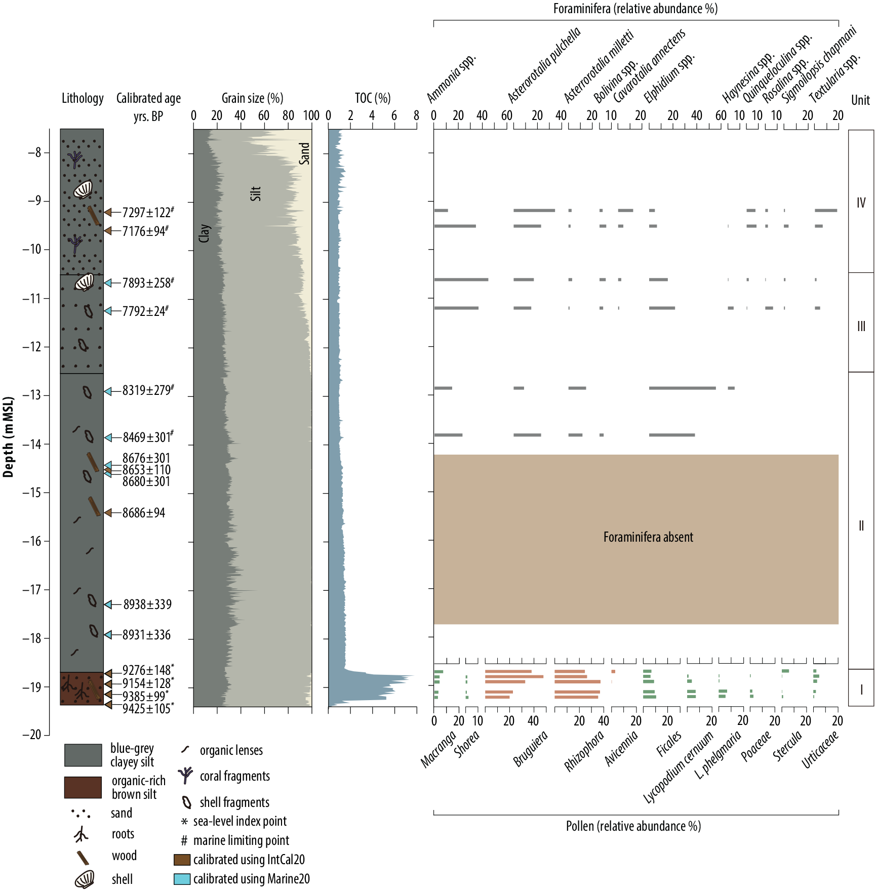
Lithology of core MSBH01B with calibrated ¹⁴C ages, grain-size and total organic carbon percentages shown. Relative foraminiferal abundances (genera/species abundance >2%) are shown corresponding to dated horizons. Relative pollen abundances are shown for mangrove (orange bars) and non-mangrove (green bars) species.

Analysis of Holocene sediments

We measured grain size and Total Organic Carbon (TOC) at 2 cm resolution to establish stratigraphic facies variation and estimate sediment compaction. For grain size, approximately 10 g of each sample was pre-treated with 10 v/v% hydrochloric acid (HCl) and 15 v/v% hydrogen peroxide (H₂O₂) to remove carbonate and organic matter, as well as to disassociate clays (Switzer and Pile, 2015). Subsequently, we performed particle-size analysis using a Malvern Mastersizer 2000 where samples were first sonicated for 60 seconds and three replicates averaged (Blott et al., 2004; Ryżak and Bieganowski, 2011). For TOC, sediment samples were milled and acidified (HCl conc. 5%) before centrifuging (at least four washes) and dried at 60^oC. We weighed ~15 mg of sample that was placed in tin capsules before loading onto an autosampling plate. TOC was determined using a Costech Elemental Analyzer (e.g. Wurster et al., 2013).

We performed microfossil (pollen and foraminiferal) analyses to determine the depositional environment of core MSBH01B, a prerequisite to estimating the indicative meaning (Horton et al., 2000; Shennan, 1986; van de Plassche, 1986). We performed pollen analysis on five samples from the organic unit from core MSBH01B. The samples were pre-treated by first adding sodium pyrophosphate (Na₄P₂O7), which removes clay by acting as a deflocculant. Subsequent centrifuging removed additional clay particles that remain in suspension. The samples were then washed with potassium hydroxide (KOH) to remove humic acids by bringing them into solution. Samples were then sieved and washed with 10% HCl to remove carbonates. Acetolysis was performed to remove polysaccharides and help increase the contrast of ornamentation on pollen grains. Mineral fragments were then removed from organic particles through heavy liquid separation using sodium polytungstate, [Na₆(H₂W₁₂O₄₀)] at a density of 2.0 (Brown, 2008). Finally, samples were mounted on slides using glycerol before identifying pollen grains under a microscope. We counted at least 300 pollen grains per slide to assure representation of taxa. Once counts were completed, we calculated relative percent abundance and Shannon-Weiner Diversity. We then assessed the taxa present to identify the paleoenvironment (i.e. Hassan, 1989; Horton et al., 2005).

We performed foraminiferal analysis on 12 samples from the blue-grey mud. These samples correspond to depths in the core where macrofossil radiocarbon samples were also obtained. Sediment from each sample was wet sieved through stacked 500 and 63 μm sieves. The coarser residuals on the 500 μm sieve were inspected under the binocular microscope for foraminiferal specimens before discarding the debris. Identification was performed under a binocular microscope with wet samples. At least 200 foraminiferal individuals were counted if possible; otherwise, the whole sample was counted. Reference for foraminiferal taxonomy followed modern foraminiferal studies from proximal areas in Peninsular Malaysia (e.g. Martin et al., 2018; Minhat et al., 2016; Suriadi et al., 2019).

Reconstructing the elevation and age of former sea-levels

To estimate RSL for core MSBH01B and other published sea-level data (Bird et al., 2007, 2010), the indicative meaning must be defined (Shennan, 2015). The indicative meaning comprises the indicative range (IR), which is the vertical range of the proxy’s relationship with tide levels, and the reference water level (RWL) or central tendency of the indicative range (Horton et al., 2000; Shennan, 1986; van de Plassche, 1986).

We used the microfossil data from core MSBH01B and the metadata from Bird et al. (2007, 2010) to assign the indicative meanings (Table 1). The Bird et al. (2007, 2010) data is obtained from mangrove, marine and intertidal environments whose depositional environment was determined from the lithology. The radiocarbon dates are derived from wood and shell material found in basal bleached clays, organic-rich mangrove peats and shelly sandy clays. We adopt a conservative indicative range of MTL to HAT for mangrove-derived samples (e.g. Khan et al., 2017; Mann et al., 2019) than Bird et al. (2007, 2010), which has been supported by local studies that have observed mangroves to colonize the upper intertidal zone between MTL and MHWST (Ng et al., 1999).

Table 1.

Definition of the indicative meanings for different indicator types implemented in this study to calculate RSL in order to develop the Singapore database.

Sample type	Evidence	Reference water level	Indicative range
Index points
Mangrove environment	Sedimentological information, in situ shells and plant macrofossils, mangrove pollen (>40% abundance), referring to a general mangrove environment (Bird et al., 2007, 2010; Hesp et al., 1998; this study).	(HAT to MTL)/2	HAT to MTL
Limiting points
Marine limiting	Plant macrofossils and shells within sub-laminated marine muds (identified by presence of benthic subtidal foraminifera) (Bird et al., 2010; this study). In-situ marine shells without species description and microfossil assemblages. Found in sandy and silty sediments typical of mudflat, lagoonal, upper shoreface, prodelta or marine environments (Bird et al., 2007, 2010; Hesp et al., 1998). In-situ corals (Bird et al., 2007, 2010; Hesp et al., 1998).	MTL	Below MTL

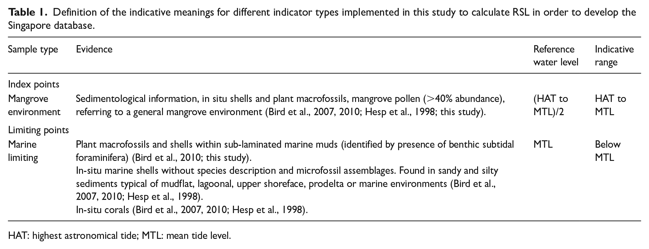
HAT: highest astronomical tide; MTL: mean tide level.

Where microfossil and/or metadata data indicated formation and deposition in marine environments, the sample was classified as a limiting date (Engelhart et al., 2011). Limiting data cannot be used to produce SLIPs but RSL must fall above marine limiting dates (Mann et al., 2019). We define the reference water level as MTL, and the indicative range as below MTL, for two main types of marine limiting data: plant macrofossils and marine shells found within marine sediments; and in-situ corals.

A significant uncertainty for the vertical position of RSL is sediment compaction, especially for early Holocene sediments with substantial sediment overburden (e.g. Törnqvist et al., 2008; Horton and Shennan, 2009). The data from Bird et al. (2007) have been previously corrected for autocompaction following the methodology of Bird et al. (2004). We used the same methodology to correct the elevation of SLIPs and limiting dates of Core MSBH01B. Bird et al. (2004) calculated compaction rates by comparison of the dry bulk density, total organic carbon (TOC) and grain-size parameters of a compacted sample with the uncompacted dry bulk density of modern sediment samples with the same TOC and grain-size characteristics. Following Bird et al. (2004), we predict the initial uncompacted dry bulk density of samples at 2-cm resolution within core MSBH01B using the following equation:

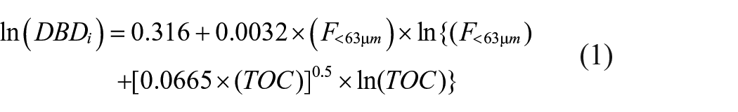
\begin{matrix} \ln (D B D_{i}) = 0.316 + 0.0032 \times (F_{< 63 μ m}) \times \ln {(F_{< 63 μ m}) \\ + {[0.0665 \times (T O C)]}^{0.5} \times \ln (T O C)} \end{matrix}

(1)

where DBD_i is the initial uncompacted dry bulk density of the sample; F_{<63 μm} is the combined silt and clay percentage of the sample; and TOC is the total organic carbon of the sample (Bird et al., 2004).

We calculated the sediment compaction correction for sediments below each SLIP/limiting data s for each 2 cm interval using the following equation:

S C_{s} = \sum [0.02 m x (D B D_{s} - D B D_{i}) / D B D_{s}]

(2)

where SC_s is the sediment compaction correction of SLIP/limiting date s; DBD_s is the compacted dry bulk density of the sample.

The RSL for each SLIP and limiting date is calculated using the following equation:

{RSL}_{s} {= E}_{s} - {RWL}_{s} {+ SC}_{s}

(3)

where E_s refers to the elevation of SLIP/limiting date s, and RWL_s refers to the reference water level of the SLIP/limiting date s. Both are expressed relative to the same datum (e.g. MSL). SC_s is the sediment compaction correction of SLIP/limiting data s.

We selected 16 wood, charcoal, and shell (bivalves and gastropods only) samples from core MSBH01B to estimate the age of SLIPs/limiting dates. All samples were cleaned with deionized water and sonicated at least three times to remove sediment and other impurities following the methods of Kemp et al. (2013). Samples were sent to Rafter Radiocarbon Laboratory, GNS Science in New Zealand for further pre-treatment (acid-alkali-acid) and Accelerator Mass Spectrometry (AMS) ¹⁴C dating (Baisden et al., 2013). We calibrated radiocarbon dates from core MSBH01B and published studies of Bird et al. (2007, 2010) using IntCal20 (Reimer et al., 2020) and Marine20 curves (Heaton et al., 2020) in Calib 8.20 (Stuiver, et al., 2020). We calculated ΔR, a regional correction to the globally averaged marine reservoir effect (Heaton et al., 2020), from a paired in situ bivalve-wood sample from −14.48 m MSL in core MSBH01B following Reimer and Reimer (2017). The deltar application (Reimer and Reimer, 2017) calculates ΔR and its uncertainty by first calibrating the terrestrial radiocarbon age from the piece of wood with the calibration curve. Deltar then reverse calibrates discrete points of the resulting probability density function (pdf) with the marine calibration curve. A convolution integral is used to determine a confidence interval for the offset between the radiocarbon dated bivalve marine sample and the reverse-calibrated pdf of the atmospheric sample (Reimer and Reimer, 2017).

Uncertainty of the vertical position of RSL

The total vertical uncertainty for each SLIP and limiting date is estimated from the indicative range and a variety of factors inherent in the collection and processing of samples for sea-level research (Engelhart and Horton, 2012; Hijma et al., 2015; Shennan and Horton, 2002) (Table 2). Total uncertainty for each sample (E_i) was estimated from the expression:

E_{i} = {({e^{2}}_{1} + {e^{2}}_{2} + & + {e^{2}}_{n})}^{1 / 2}

(4)

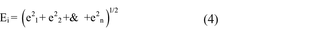
where e₁. . .e_n are individual sources of error for sample i (Shennan and Horton, 2002). Estimating palaeotidal range variation is beyond the scope of this study.

Table 2.

Standardized vertical uncertainties adopted for the construction of the Singapore database.

Sources of uncertainty	Description
Uncertainties related to the indicative meaning of a sample
Indicative range uncertainty	±Indicative range/2
Uncertainties related to the determination of the depth of a sample in a core
Sample thickness uncertainty*	±Sample thickness/2
Sampling uncertainty	±0.01 m
Core shortening/stretching uncertainty	±0.15 m for rotary coring
Core shortening/stretching uncertainty	±0.05 m for hand coring
Non-vertical drilling uncertainty	0.02 m/m depth
Uncertainties related to the determination of the elevation of a core
Offshore sample collection
Tidal uncertainty	±Tidal range/2
Water depth uncertainty	±0.5 m
High-precision surveying methods
Total station uncertainty	±0.01 m
GPS or RTK uncertainty	±0.1 m
Benchmark uncertainty	±0.1 m

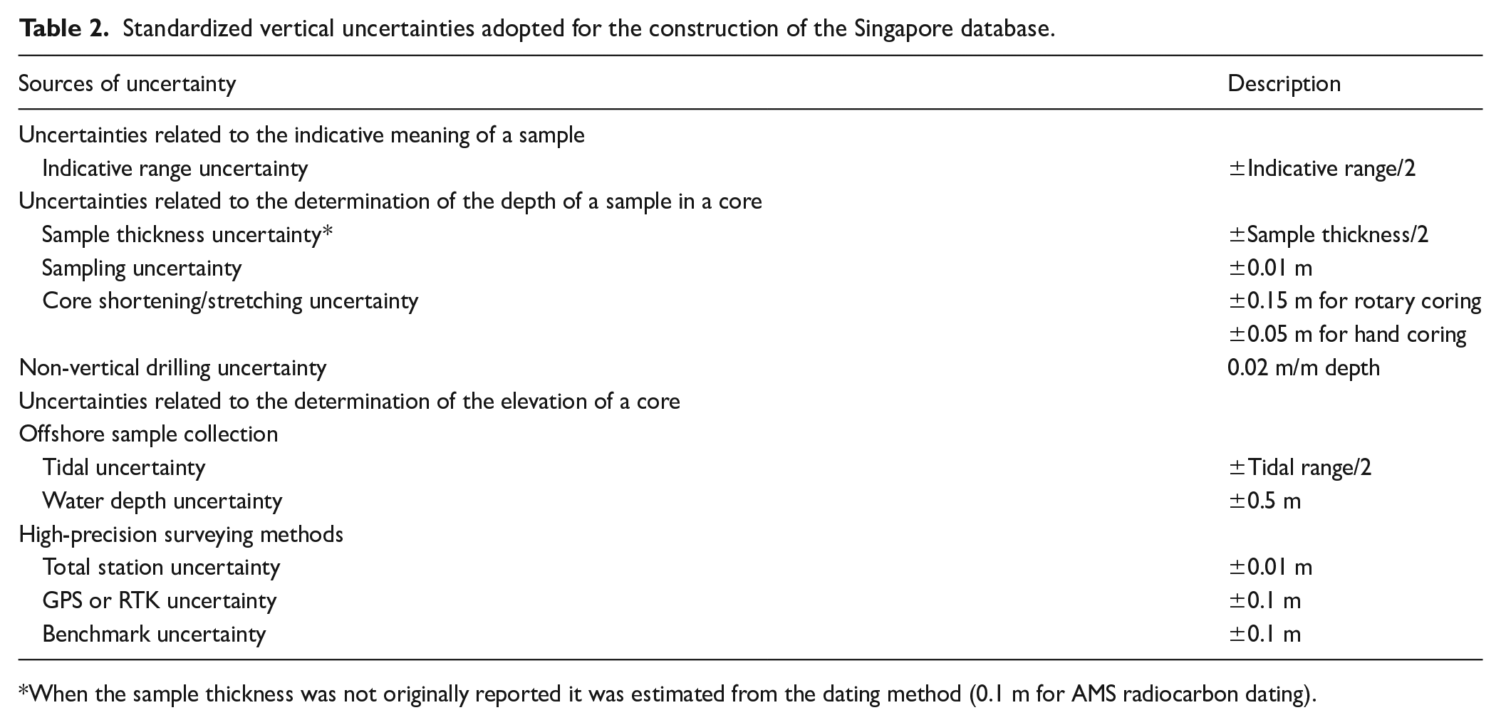
When the sample thickness was not originally reported it was estimated from the dating method (0.1 m for AMS radiocarbon dating).

Quantitvative modelling of relative sea level and glacial isostatic adjustment

To estimate RSL for Singapore we combined the data from core MSBH01B and Bird et al. (2007, 2010). We subsequently applied the Error-In-Variables Integrated Gaussian Process (EIV-IGP) model of Cahill et al. (2015) to derive quantitative RSL trends while incorporating vertical and temporal uncertainties of the SLIPs. The EIV-IGP model does not include limiting points. The EIV (errors-in-variables) approach (Dey et al., 2000) accounts for error due to radiocarbon age uncertainties, and the IGP (integrated Gaussian process) is useful for modelling non-linear trends in data. The EIV-IGP model calculates the behaviour and rate of RSL change over time by placing a Gaussian process prior specified by a mean function and a covariance function that smooths the RSL reconstructions.

We compared the RSL reconstructions for the Singapore region and a subset of the regional database of Southeast Asia, Maldives, India and Sri Lanka (SEAMIS) (Mann et al., 2019) with the latest iteration of GIA models (Li and Wu, 2019; Peltier et al., 2015). We estimated the GIA response of a spherical, self-gravitating, materially compressible Maxwell Earth using the Coupled Laplace-Finite Element (CLFE) method (Wu, 2004). The effects of rotational feedback and time dependent ocean margin were also included in the computation. The finite grid has a 0.5 × 0.5-degree spatial resolution near the surface but decreases with depth to reduce the computation time. We used the 3D Earth model HetM-LHL140 (Li and Wu, 2019), coupled with the ICE-6G_C (Peltier et al., 2015) surface loading history model, to provide the RSL predictions. The 3D Earth model HetM-LHL140 includes lateral variations both in the lithospheric thickness and mantle viscosity, and has been tuned to fit deglacial RSL data, present-day rate of vertical land motion and gravity-rate-of-change data in North America and Fennoscandia simultaneously (Li and Wu, 2019; Peltier et al., 2015).

Results

Litho-, bio- and chronostratigraphy of Core MSBH01B

The surface elevation of core MSBH01B is 4.1 m MSL and the top ~12 m is identified as surface fill material. We subdivided the Holocene sediments into four lithological units (Figure 2), which overlay a highly oxidised, weathered, incompressible stiff clay unit, interpreted as sub-aerially exposed, desiccated MIS 5 marine clay (Bird et al., 2007; Chua et al., 2020). Unit I is a dark brown, organic-rich medium-fine sandy silt from −19.4 to −18.7 m MSL, dominated by terrestrial macrofossils (wood, bark and root). Unit I grades gradually over 5 cm into Unit II (−18.7 to −12.6 m MSL), which is a greenish grey-to-grey homogenous, clayey silt with occasional shells and organic lenses. Unit III overlies Unit II at a depth of −12.6 to −10.5 m MSL. It consists of blue-grey medium-fine silt with few shell fragments. Unit IV overlies Unit III and is found between −10.5 and −7.5 m MSL where it is truncated by surface fill material. Unit IV is comprised of grey-brown, very coarse silt-medium silt with frequent shell and coral fragments.

Pollen analysis of Unit I revealed an assemblage dominated by mangrove pollen (Figure 2). We assumed that samples with over 40% mangrove pollen represent mangrove swamps (e.g. Hassan, 1989; Horton et al., 2005). Consistently high amounts of mangrove pollen are present across all five samples between −19.3 and −18.8 m MSL. The percentage abundance of total mangrove pollen ranged from 55% to 74% and the samples all had a low to moderate diversity (1.67–2.13) of pollen taxa. The dominant species observed in Unit I are mangrove taxa such as Bruguiera (32% ± 10%) and Rhizophora (32% ± 5%). Greater abundance of Rhizophora pollen found at the lower part of Unit I (19.3–19.0 m MSL), coupled with higher diversity, suggests a deltaic or estuarine environment (Hassan, 1989). The presence of some freshwater taxa, such as Macaranga and Shorea and grasses suggest that there were other types of environments, such as freshwater wetlands and grasslands, located nearby; however, the low abundance of any of these taxa indicates that these environments were not present at the sampling location (Hassan, 1989).

A total of 113 foraminiferal species belonging to 30 genera were identified and comprise predominantly calcareous benthic foraminifera. Foraminifera are absent in Units I and II between −18 and −14 m MSL (Figure 2) suggesting possible taphonomic impacts resulting in poor preservation of foraminifera tests which are common on tropical intertidal environments (Berkeley et al., 2007). Foraminifera present in Units II–IV are dominated by three different assemblages. The assemblage of the uppermost part of Unit II was comprised of Elphidium spp. (47.2 ± 8.7%), Asterorotalia pulchella (16.0% ± 7.1%) and Ammonia spp. (18.9% ± 4.2%). The assemblage in Unit III had increased relative abundance of Ammonia spp. (44.0% ± 6.0%) and decreased relative abundance in Elphidium spp. (19.3% ± 2.5%) and Asterorotalia pulchella (11.2% ± 6.6%). The foraminiferal assemblages observed in Units II and III are comparable to modern subtidal assemblages found at the eastern coast of Johor, Malaysia, where water depths are less than 20 m (Minhat et al., 2016). Ammonia and Elphidium are found mainly in sheltered, shallow marine, slightly brackish environments and widespread in the eastern coast of Peninsular Malaysia (Suriadi et al., 2019). The assemblage in Unit IV is dominated by Asterorotalia pulchella (28.7% ± 6.0%), Ammonia spp. (22.5% ± 11.6%) with common species Textularia spp. (12.6% ± 6.0 %), Cavarotalia annectens (8.4% ± 4.2%) and Quinqueloculina spp. (7.9% ± 0.6%). This assemblage displays higher species diversity and comprise common species recovered from subtidal sediments of Johor characterizing the typical tropical shallow marine environments. The increase in abundance of the agglutinated species Textularia imply greater water depths (>20 m) (Minhat et al., 2016).

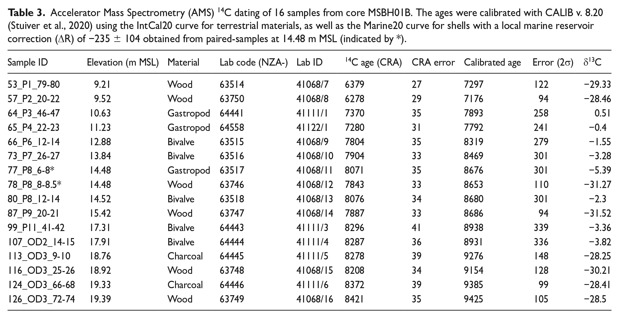
We generated 16 radiocarbon dates from −19.4 to −9.2 m MSL with no age reversals with respect to the uncertainty of the calibrated ages (Table 3). We applied a local marine reservoir correction to the eight shell dates using paired bivalve-wood samples from −14.48 m MSL, which indicates a ∆R of −235 ± 104 years (Reimer and Reimer, 2017). This value is similar to the average ∆R of −193 ± 84 years from pre-bomb bivalve shells from Singapore (Heaton et al., 2020; Southon et al., 2002) and −278 ± 139 years from Geylang (Bird et al., 2007; Heaton et al., 2020; Reimer and Reimer, 2020). After calibration, the eight shell dates provided ages between 9266–8595 and 8151–7635 cal. yrs. BP. Four dates from wood and charcoal in Unit I produced ages between 9529–9320 and 9423–9128 cal. yrs. BP. The 12 dates from Units II-IV provided ages between 9266–8595 and 7270–7082 cal. yrs. BP.

Table 3.

Accelerator Mass Spectrometry (AMS) ¹⁴C dating of 16 samples from core MSBH01B. The ages were calibrated with CALIB v. 8.20 (Stuiver et al., 2020) using the IntCal20 curve for terrestrial materials, as well as the Marine20 curve for shells with a local marine reservoir correction (ΔR) of −235 ± 104 obtained from paired-samples at 14.48 m MSL (indicated by *).

Sample ID	Elevation (m MSL)	Material	Lab code (NZA-)	Lab ID	¹⁴C age (CRA)	CRA error	Calibrated age	Error (2σ)	δ¹³C
53_P1_79-80	9.21	Wood	63514	41068/7	6379	27	7297	122	−29.33
57_P2_20-22	9.52	Wood	63750	41068/8	6278	29	7176	94	−28.46
64_P3_46-47	10.63	Gastropod	64441	41111/1	7370	35	7893	258	0.51
65_P4_22-23	11.23	Gastropod	64558	41122/1	7280	31	7792	241	−0.4
66_P6_12-14	12.88	Bivalve	63515	41068/9	7804	35	8319	279	−1.55
73_P7_26-27	13.84	Bivalve	63516	41068/10	7904	33	8469	301	−3.28
77_P8_6-8*	14.48	Gastropod	63517	41068/11	8071	35	8676	301	−5.39
78_P8_8-8.5*	14.48	Wood	63746	41068/12	7843	33	8653	110	−31.27
80_P8_12-14	14.52	Bivalve	63518	41068/13	8076	34	8680	301	−2.3
87_P9_20-21	15.42	Wood	63747	41068/14	7887	33	8686	94	−31.52
99_P11_41-42	17.31	Bivalve	64443	41111/3	8296	41	8938	339	−3.36
107_OD2_14-15	17.91	Bivalve	64444	41111/4	8287	36	8931	336	−3.82
113_OD3_9-10	18.76	Charcoal	64445	41111/5	8278	39	9276	148	−28.25
116_OD3_25-26	18.92	Wood	63748	41068/15	8208	34	9154	128	−30.21
124_OD3_66-68	19.33	Charcoal	64446	41111/6	8372	39	9385	99	−28.41
126_OD3_72-74	19.39	Wood	63749	41068/16	8421	35	9425	105	−28.5

Reconstruction of sea-level index points and limiting data

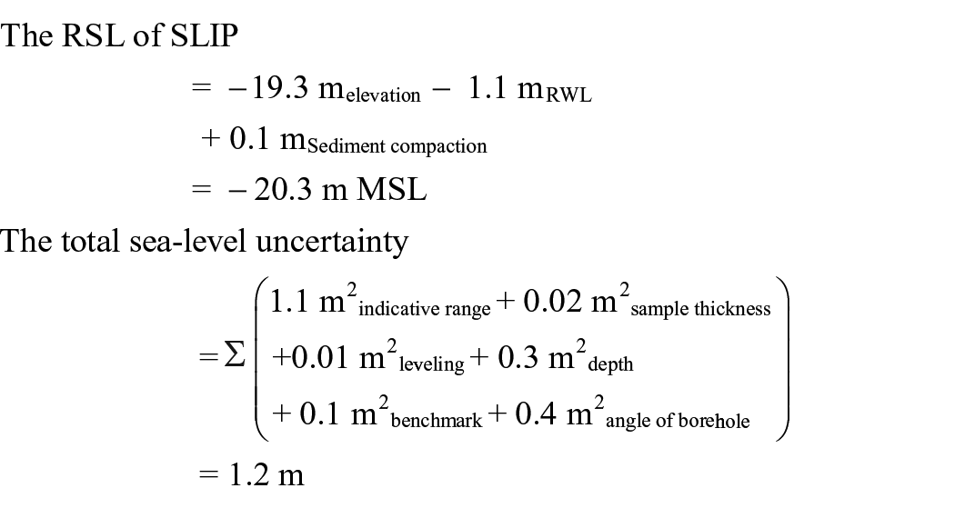
We produced four SLIPs and six marine limiting data from core MSBH01B where there was microfossil evidence to define the indicative meaning (Table 4). For example, we selected a piece of charcoal from basal mangrove peat (Unit I) from −19.3 m MSL revealing a ¹⁴C age of 8372 ± 39 (1σ) years which was subsequently calibrated to 9483–9286 cal. yrs. BP. The pollen assemblage indicates the presence of mangroves (e.g. Hassan, 1989; Horton et al., 2005), thus the SLIP formed between HAT and MTL (1.1 ± 1.1 m MSL). We corrected the elevation of −19.3 m MSL for 0.1 m of compaction.

\begin{matrix} The RSL of SLIP \\ = - 19.3 m_{elevation} - 1.1 m_{RWL} \\ + 0.1 m_{Sediment compaction} \\ = - 20.3 m MSL \\ The total sea - level uncertainty \\ = Σ (\begin{array}{l} 1.1 {m^{2}}_{indicative range} + 0.02 {m^{2}}_{sample thickness} \\ + 0.01 {m^{2}}_{leveling} + 0.3 {m^{2}}_{depth} \\ + 0.1 {m^{2}}_{benchmark} + 0.4 {m^{2}}_{angle of borehole} \end{array}) \\ = 1.2 m \end{matrix}

Table 4.

Eighty-eight sea-level data points (64 SLIPs and 24 limiting dates) forming the Singapore sea-level database.

Sea-level index points
Sample	Location	Lab prefix	Lab code	Dated material	¹⁴C age	1σ error	Age range (calibrated)			RSL (m MSL)	2σ error	Citation
GEY PS1 72 cm	Geylang	ANUA	25708	Wood	1301	192	791	−	1567	−2.27	1.10	Bird et al. (2010)
GEY PS17 19 cm	Geylang	ANUA	25710	Root	8020	49	8650	−	9019	−16.21	1.12	Bird et al. (2007)
KCD 14 +20 cm	Kim Chuan Depot	ANU	11799	Wood	7340	70	8016	−	8326	−3.08	1.10	Bird et al. (2007)
KCD 4 +90 cm	Kim Chuan Depot	ANUA	11804	Wood	5610	120	6121	−	6721	0.51	1.10	Bird et al. (2007)
KCD 6 +60 cm	Kim Chuan Depot	ANUA	11807	Bark	5270	170	5611	−	6392	0.51	1.10	Bird et al. (2007)
KCD 7 +10 cm	Kim Chuan Depot	ANUA	11814	Wood	5340	110	5901	−	6389	2.27	1.10	Bird et al. (2007)
KCD-12 0 cm	Kim Chuan Depot	ANU	11809	Wood	6140	90	6792	−	7253	0.15	1.10	Bird et al. (2007)
KCD-13 +15 cm	Kim Chuan Depot	ANU	11810	Wood	6190	70	6901	−	7257	0.47	1.10	Bird et al. (2007)
KCD-13 −120 cm	Kim Chuan Depot	ANU	11811	Wood	7070	130	7668	−	8170	−0.97	1.10	Bird et al., 2007
KCD-13 −125 cm	Kim Chuan Depot	ANU	11812	Wood	6650	80	7425	−	7663	−1.09	1.10	Bird et al. (2007)
KCD-14 +35 cm	Kim Chuan Depot	ANU	12048	Wood	7000	80	7679	−	7965	−2.93	1.10	Bird et al. (2007)
KCD-1B	Kim Chuan Depot	ANU	11800	Wood	6750	80	7433	−	7742	−2.22	1.10	Bird et al. (2007)
KCD-1E	Kim Chuan Depot	ANU	11801	Wood	5890	110	6413	−	6982	−0.44	1.10	Bird et al. (2007)
KCD-4D 0 cm	Kim Chuan Depot	ANU	11802	Wood	6200	90	6856	−	7309	−0.42	1.10	Bird et al. (2007)
KCD-4E −10 cm	Kim Chuan Depot	ANU	11803	Wood	6000	60	6675	−	6986	−0.52	1.10	Bird et al. (2007)
KCD-6 +25 cm	Kim Chuan Depot	ANUA	26403	Wood	6118	42	6890	−	7158	0.16	1.10	Bird et al. (2007)
KCD-6 +30 cm	Kim Chuan Depot	ANU	11806	Wood	6300	80	7000	−	7421	0.21	1.10	Bird et al. (2007)
LCK 4-1-4	Lim Chu Kang	ANUA	25705	Wood	1879	191	1390	−	2305	−1.47	1.10	Bird et al. (2007)
LCK-1 0 cm	Lim Chu Kang	ANUA	22221	Wood	2397	191	1944	−	2871	−1.13	1.10	Bird et al. (2007)
LCK-4-3 4 cm	Lim Chu Kang	SSAMS	4605	Wood	6951	47	7681	−	7922	−3.16	1.10	Bird et al. (2007)
113_OD3_9-10	Marina South	NZA	64445	Wood	8278	39	9128	−	9423	–18.16	1.42	This Study
116_OD3_25-26	Marina South	NZA	63748	Wood	8208	34	9026	−	9282	–18.74	1.30	This Study
124_OD3_66-68	Marina South	NZA	64446	Wood	8372	39	9286	−	9483	–20.28	1.13	This Study
126_OD3_70-72	Marina South	NZA	63749	Wood	8421	35	9320	−	9529	−20.52	1.13	This study
NIE 4	National Institute of Education	ANUA	24303	Wood	5040	184	5329	−	6267	3.67	1.09	Bird et al. (2007)
NIE 5	National Institute of Education	ANUA	24304	Wood	4949	187	5299	−	6187	3.88	1.09	Bird et al. (2007)
STA-1 −10 cm A	National Stadium	ANU	11996	Wood	7910	100	8479	−	9012	−9.76	1.12	Bird et al. (2007)
STA-1 −10 cm B	National Stadium	ANU	11976	Wood	7920	80	8553	−	8998	−9.76	1.12	Bird et al. (2007)
STA-1 −30 cmB hp	National Stadium	ANUA	26330	Wood	7699	45	8404	−	8588	−10.19	1.11	Bird et al. (2007)
BBP 140302	Singapore Management University	ANUA	22228	Wood	6673	41	7433	−	7613	−2.06	1.10	Bird et al. (2007)
BBP-2 205 cm	Singapore Management University	ANUA	19525	Wood	5990	47	6678	−	6948	1.15	1.24	Bird et al. (2007)
BBP-2 407 cm	Singapore Management University	ANUA	19526	Wood	6199	42	6964	−	7248	−2.38	1.10	Bird et al. (2007)
BBP-2 430cm	Singapore Management University	ANUA	19527	Wood	6503	63	7280	−	7561	−2.67	1.10	Bird et al. (2007)
SMU-1 0 cm A	Singapore Management University	ANU	11989	Wood	7470	160	7970	−	8587	−3.72	1.10	Bird et al. (2007)
SMU-1 0 cm B	Singapore Management University	ANUA	26328	Wood	7059	43	7790	−	7968	−3.72	1.10	Bird et al. (2007)
SMU-11 +20 cm	Singapore Management University	ANU	11994	Wood	7380	100	8012	−	8378	−1.92	1.10	Bird et al. (2007)
SMU-2A	Singapore Management University	ANU	11988	Wood	6650	110	7323	−	7689	−3.12	1.10	Bird et al. (2007)
SMU-2B	Singapore Management University	ANU	11982	Wood	7150	90	7791	−	8173	−3.27	1.10	Bird et al. (2007)
SMU-3 +40 cm	Singapore Management University	ANU	11983	Wood	7070	90	7690	−	8025	−3.94	1.10	Bird et al. (2007)
SMU-3 +80 cm A	Singapore Management University	ANU	11985	Wood	6360	240	6677	−	7672	–3.52	1.10	Bird et al. (2007)
SMU-3 +80 cm B	Singapore Management University	ANU	11987	Wood	7160	320	7367	−	8630	−3.52	1.10	Bird et al. (2007)
SMU-4 – 40 cmA hp	Singapore Management University	ANUA	26404	Wood	7359	193	7792	−	8542	−5.02	1.10	Bird et al. (2007)
SMU-4 0 cm	Singapore Management University	ANU	11981	Wood	6500	270	6789	−	7922	−4.54	1.10	Bird et al. (2007)
SMU-4 10 cm	Singapore Management University	ANU	11984	Wood	6950	180	7435	−	8167	−4.65	1.10	Bird et al. (2007)
SMU-8 +100 (borer)	Singapore Management University	ANU	11986	Wood	7590	55	8217	−	8537	−6.52	1.10	Bird et al. (2007)
SMU-8 +100 cm	Singapore Management University	GU	11246	Wood	7640	190	8036	−	8982	−6.52	1.10	Bird et al. (2007)
SMU-8 +10 cm A	Singapore Management University	ANU	11980	Wood	7660	130	8179	−	8969	−7.52	1.10	Bird et al. (2007)
SMU-8 +10 cm B	Singapore Management University	ANU	11990	Wood	7820	90	8418	−	8981	−7.52	1.10	Bird et al. (2007)
SMU-9 +30 cm	Singapore Management University	ANU	11992	Wood	7640	80	8220	−	8595	−6.774	1.10	Bird et al. (2007)
SMU-9 +40 cm	Singapore Management University	ANU	11993	Wood	7350	100	7978	−	8363	−6.87	1.10	Bird et al. (2007)
SMU-9 +90 cm A	Singapore Management University	ANU	11991	Wood	7176	48	7869	−	8165	−6.37	1.10	Bird et al. (2007)
SMU-9 +90 cm B	Singapore Management University	ANU	11977	Wood	7270	220	7668	−	8518	−6.37	1.10	Bird et al. (2007)
SBU 1-2-8	Sungei Buloh	ANUA	22726	Wood	7017	43	7734	−	7940	−3.60	1.09	Bird et al. (2007)
SBU-1 1-3	Sungei Buloh	ANUA	22729	Wood	6415	40	7267	−	7423	−1.27	1.15	Bird et al. (2007)
SBU-1 1-7	Sungei Buloh	ANUA	22728	Wood	6723	49	7505	−	7674	−1.90	1.12	Bird et al. (2007)
SBU-1 2-1	Sungei Buloh	ANUA	22727	Wood	6683	60	7431	−	7662	−2.40	1.11	Bird et al. (2007)
SBU3-1-6	Sungei Buloh	ANUA	22730	Wood	2241	200	1748	−	2743	−0.02	1.09	Bird et al. (2007)
Shell (Hesp)	Sungei Nipah	BETA	78261	Shell	7690	50	7939	−	8476	−10.71	1.11	Hesp et al. (1998) (reviewed by Bird et al., 2007)
Wood (Hesp)	Sungei Nipah	BETA	78262	Wood	7790	60	8416	−	8753	−11.52	1.11	Hesp et al. (1998) (reviewed by Bird et al., 2007)
MAR-3 −195 cm	Suntec City	ANU	11842	Wood	7800	90	8406	−	8980	−8.60	1.10	Bird et al. (2007)
MAR-3A −145 cm	Suntec City	ANU	11843	Wood	7740	100	8350	−	8974	−7.82	1.11	Bird et al. (2007)
MAR-4 −205 cm	Suntec City	ANU	11839	Wood	7340	110	7967	−	8367	−7.89	1.11	Bird et al. (2007)
MAR-5 +40 cm	Suntec City	ANU	11840	Wood	7650	100	8202	−	8636	−8.54	1.10	Bird et al. (2007)
MAR-5 +75 cm	Suntec City	ANU	11841	Wood	7530	80	8174	−	8518	−7.81	1.11	Bird et al. (2007)

Marine Limiting
Sample	Location	Lab prefix	Lab code	Dated material	¹⁴C age	1σ error	Age range (calibrated)			RSL (m MSL)	2σ error	Citation
GEY PS3 78-84	Geylang	GU	17983	Bivalve	5775	30	5945	−	6495	−3.04	0.22	Bird et al. (2007)
GEY PS4 68-76	Geylang	GU	17885	Gastropod	6035	30	6254	−	6794	−3.90	0.22	Bird et al. (2007)
GEY PS5 69 cm (shell)	Geylang	GU	11247	Oyster	6160	45	6357	−	6949	−4.74	0.22	Bird et al. (2007)
GEY PS6 56–61 cm (shell)	Geylang	GU	17650	Bivalve	6275	35	6487	−	7086	−5.49	0.22	Bird et al. (2007)
GEY PS7 19–26	Geylang	GU	17651	Bivalve	6430	30	6678	−	7236	−6.04	0.22	Bird et al. (2007)
GEY PS8 19–26	Geylang	GU	17653	Bivalve	6730	30	7003	−	7510	−6.94	0.22	Bird et al. (2007)
GEY PS8 54	Geylang	GU	17652	Bivalve	6920	30	7217	−	7684	−7.27	0.22	Bird et al. (2007)
GEY PS9 21 (gastropod)	Geylang	GU	11249	Gastropod	7365	45	7623	−	8150	−7.82	0.22	Bird et al. (2007)
GEY PS9 21 cm (wood)	Geylang	GU	11248	Wood	7095	50	7797	−	8014	−7.82	0.22	Bird et al. (2007)
GEY PS10 69	Geylang	GU	17654	Bivalve	7485	30	7746	−	8276	−9.27	0.22	Bird et al. (2007)
GEY PS11 19–26	Geylang	GU	17655	Bivalve	7260	30	7537	−	8014	−9.67	0.22	Bird et al. (2007)
GEY PS15 45 cm (shell)	Geylang	GU	11250	Bivalve	7685	50	7934	−	8470	−13.48	0.22	Bird et al. (2007)
GEY PS16 76 cm (shell)	Geylang	GU	11251	Bivalve	7970	50	8236	−	8892	−14.69	0.22	Bird et al. (2007)
GEY PS16 80 cm (wood)	Geylang	GU	11252	Wood	8050	50	8654	−	9120	−14.74	0.22	Bird et al. (2007)
GEY PS16 bottom 15 (wood)	Geylang	SSAMS	4609	Wood	7797	49	8425	−	8716	−14.68	0.22	Bird et al. (2007)
53_P1_79-80	Marina South	NZA-	63514	Wood	6379	27	7175	−	7419	−7.47	0.92	This study
57_P2_20-22	Marina South	NZA-	63750	Wood	6278	29	7082	−	7270	−7.77	0.92	This study
64_P3_46-47	Marina South	NZA-	64441	Shell	7370	35	7635	−	8151	−8.88	0.92	This study
65_P4_22-23	Marina South	NZA-	64558	Shell	7280	31	7551	−	8032	−9.48	0.92	This study
66_P6_12-14	Marina South	NZA-	63515	Shell	7804	35	8040	−	8598	−11.13	0.92	This study
73_P7_26-27	Marina South	NZA-	63516	Shell	7904	33	8168	−	8769	−12.10	0.92	This study
SEK-3	Pulau Sekudu	ANUA-	12051	Coral	4410	70	4315	−	5029	0.86	1.26	Bird et al. (2007)
SEK-4	Pulau Sekudu	ANUA-	12052	Coral	4340	70	4224	−	4926	0.86	1.26	Bird et al. (2007)
SEK-5	Pulau Sekudu	ANUA-	12053	Coral	1720	60	1068	−	1648	–1.26	1.26	Bird et al. (2007)

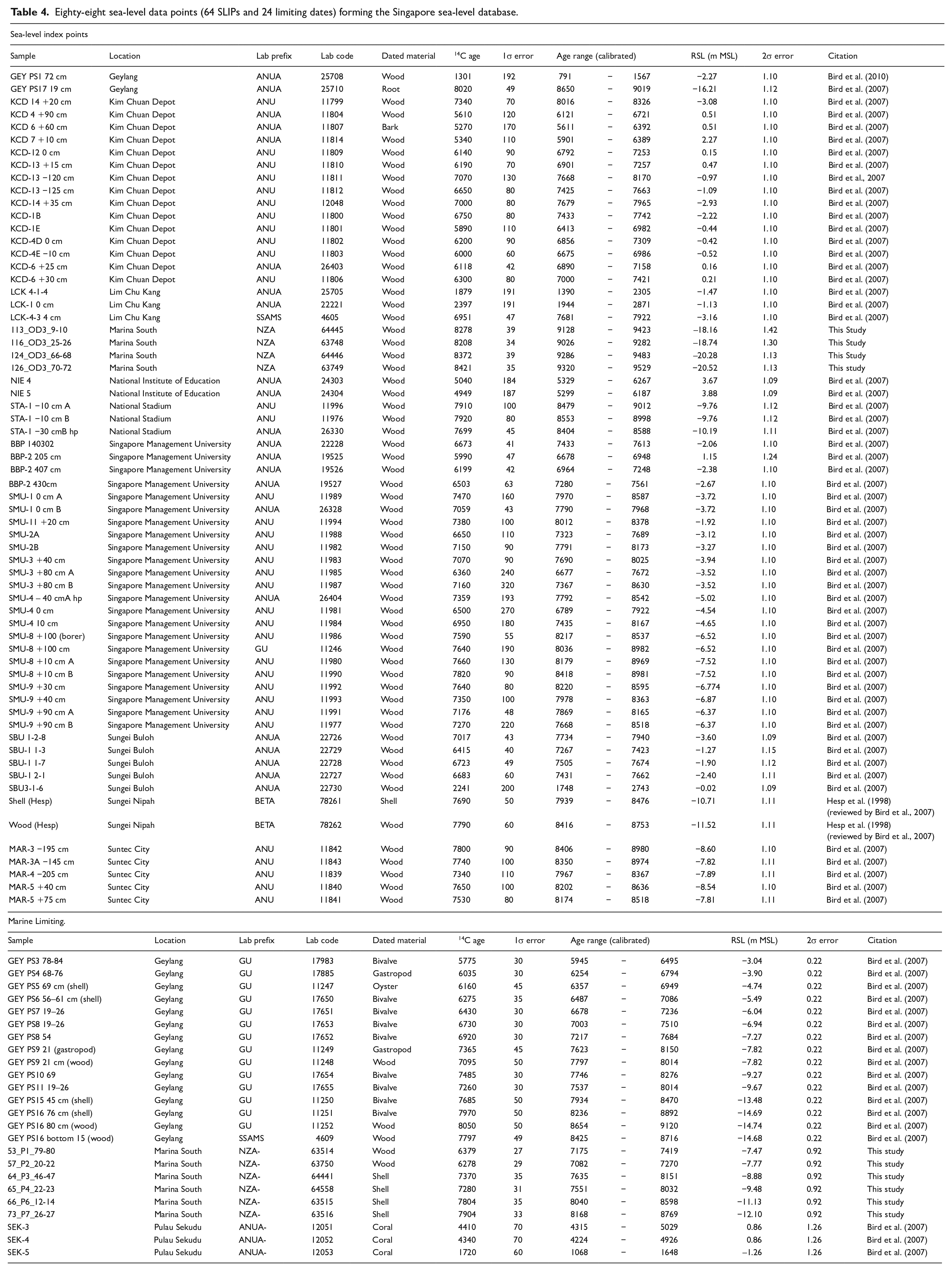
Singapore sea-level database

We validated 88 sea-level data points consisting of 64 SLIPs and 24 limiting dates (Table 4) from Bird et al. (2007, 2010), as well new data points from MSBH01B. The temporal distribution of the Holocene SLIPs is uneven with 93% between 9500 and 5600 cal. yrs. BP. The database has an absence of SLIPs between 5600 and 2500 cal. yrs. BP, but four SLIPs constrain RSL from 2500 cal. yrs. BP to present (Figure 3a).

Figure 3.

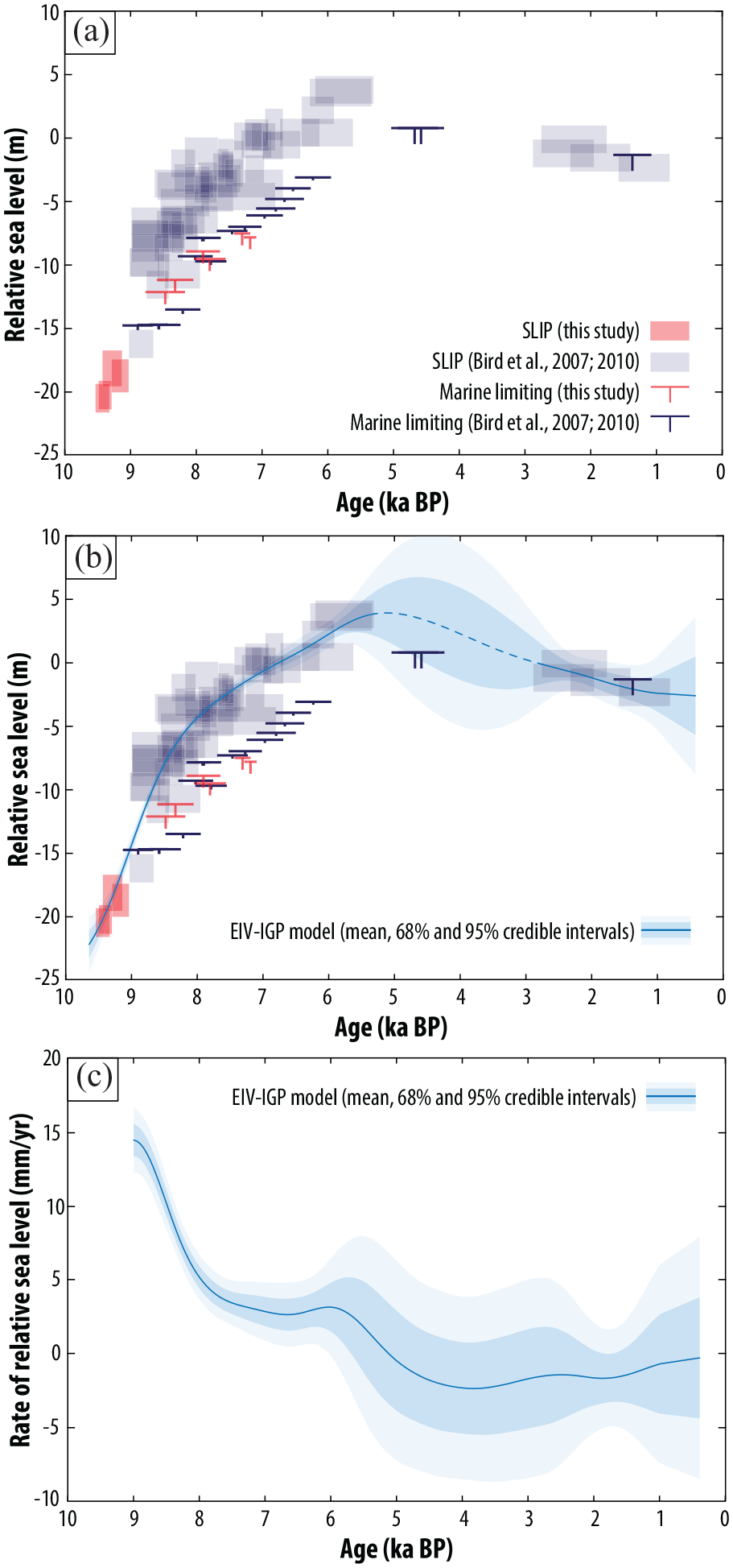
(a) Singapore relative sea-level (RSL) data comprising sea-level index points and marine limiting data. SLIPs and limiting dates from this study and Bird et al. (2007, 2010) are shown in red and blue shapes, respectively. (b) RSL data and Error-in-Variables Integrated Gaussian Process (EIV-IGP) model. Dashed line represents a period with an absence of SLIPs. (c) Rates of RSL change estimated using the EIV-IGP model.

The SLIPs show a continuous rise in RSL during the early Holocene from −21.0 to −0.7 m from ~9500 to 7000 cal. yrs. BP (Figure 3b). The rate of rise was rapid during the early Holocene reaching a maximum rise rate of 14.5 ± 2.2 mm/yr. The rate of sea-level rise subsequently decreased from an average rate of 10.2 ± 1.8 mm/yr between ~9000 and 8000 cal. yrs. BP to an average rate of 3.7 ± 1.6 mm/yr between ~8000 and 7000 cal. yrs. BP (Figure 3c). RSL continued to rise to the mid-Holocene highstand of 4.0 ± 4.5 m at 5200 cal. yrs. BP. Thereafter the mid to late-Holocene RSL is poorly constrained due to a lack of SLIPs, but two marine limiting dates suggest RSL was above 0.9 m between ~5000 and 4200 cal. yrs. BP. SLIPs from the last ~2500 years suggest RSL was near to present at 2800 cal. yrs. BP, before decreasing to −2.4 ± 2.8 m at 1000 cal. yrs. BP.

Discussion

We produced a Holocene RSL record for Singapore consisting of 88 SLIPs and limiting data, extending the reconstructions of RSL into the early Holocene. To better understand the processes controlling RSL, we compared the Singapore data with other studies (e.g. Mann et al., 2019; Tam et al., 2018) from the east coast and west coast of the Malay-Thai Peninsula (ECMP and WCMP) (Figure 1a). This Malay-Thai Peninsula database consists of 58 data points (40 SLIPs, 16 marine limiting and 2 freshwater limiting dates) that span the time interval from ~9500 to 600 cal. yrs. BP (Supplemental Appendix 1). The database shows differences in the rate of RSL change during the early and late-Holocene, and spatial variability in the magnitude and timing of the mid-Holocene highstand.

Early Holocene relative sea-level rise

The most rapid increase in RSL on the Malay-Thai Peninsula is observed in WCMP and Singapore from ~9500 to 8000 cal. yrs. BP (Figures 4b and c). The databases of WCMP and Singapore have near identical records, showing a rapid RSL rise from −21.0 to −4.4 m at average rates of ~8.4 ± 2.6 mm/yr. Such rapid RSL rise was driven by deglaciation of the Laurentide and Fennoscandian ice sheets (e.g. Lambeck et al., 2014; Stroeven et al., 2016; Ullman et al., 2016), which discharged ~20 m of sea-level equivalent into the global oceans during this period (Lambeck et al., 2014). The rates of GMSL change between 11,400 and 8200 cal. yrs. BP is higher than the regional signal of the Malay-Thai Peninsula, with Lambeck et al. (2014) predicting an average GMSL rise rate of ~15 mm/yr during this period.

Figure 4.

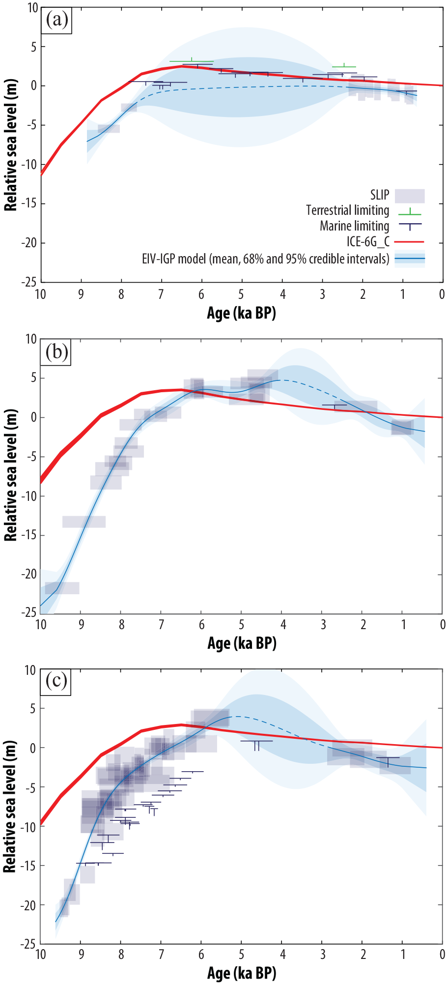
Comparison between ICE-6G_C (Peltier et al., 2015) Glacial isostatic adjustment (GIA) relative sea-level (RSL) predictions with Holocene RSL data and Error-in-Variables Integrated Gaussian Process (EIV-IGP) model for (a) east coast of the Malay-Thai Peninsula (ECMP), (b) west coast of the Malay-Thai Peninsula (WCMP) and (c) Singapore. Dashed lines represent periods with an absence of SLIPs.

Some early Holocene studies have identified a ‘stepped’ rise in GMSL (e.g. Liu et al., 2004; Hori and Saito, 2007). Indeed, in Singapore, Bird et al. (2010) identified an inflection centred upon 7600 cal. yrs. BP. Here, we used an expanded RSL database and the application of the EIV-IGP model, which is useful for non-linear modelling (Cahill et al., 2015). Using this method we do not identify an inflection, although there is a deceleration in the rate of rise from 10.2 ± 1.8 mm/yr at 8500 cal. yrs. BP to 3.0 ± 2.0 mm/yr at 7000 cal. yrs. BP (Figure 3c). The deceleration in the rate of RSL rise coincides with the final deglaciation of Fennoscandian ice sheets (e.g. Stroeven et al., 2016) and decreasing melt water input from the Laurentide (e.g. Ullman et al., 2016) and Antarctic ice sheets (e.g. Hillenbrand et al., 2017; Mackintosh et al., 2011). The presence of an inflection point centred at 7600 years BP (Bird et al., 2010) may still exist, but cannot be verified from the expanded dataset and conservative approach employed here. The debate over whether Holocene sea-level rise was oscillatory or non-monotonic in nature is not new (e.g. Fairbridge 1961; Kidson, 1982). The approach applied here, reiterates the importance of a comprehensive, standardized approach to identifying uncertainties inherent during reconstruction of RSL (Khan et al., 2019; Shennan, 1982).

The ICE-6G_C ice model, coupled with 3D Earth model HetM-LHL140, predicts a continuous, but decelerating RSL rise in Singapore and WCMP in the early Holocene, which is consistent with the trend identified from RSL reconstructions (Figure 4). Although the RSL predictions are higher in elevation compared to the early Holocene RSL reconstructions, the misfit magnitudes decrease markedly from ~15 m at 9500 cal. yrs. BP, to ~6 m in WCMP, and to ~5 m in Singapore at 8000 cal. yrs. BP, and intersects with the RSL reconstructions in both regions at ~6000 cal. yrs. BP (Figures 4b and c). The data-model difference may imply that a greater amount of ice melting is required for the later part of the deglacial period (e.g. Bradley et al., 2016). Also, subsidence of the continental shelf could possibly have contributed to the elevation misfit (e.g. Sarr et al., 2019; Tam et al., 2018). Continental shelf sediments may be affected by subsidence due to long-term (10⁷–10⁶ year) thermoflexural effects and compaction due to sediment loading and groundwater withdrawal (Horton et al., 2018). In New Jersey, thermoflexural subsidence in this region is less than 10 m/Myr (0.01 mm/yr) and subsidence due to deep (pre-Holocene) compaction is less (Miller et al., 2013). Yu et al. (2012) quantified a similar, low (<0.15 mm/yr) thermoflexural subsidence in the Mississippi delta region.

Magnitude and timing of the mid-Holocene highstand

Mid-Holocene highstands in far-field regions are attributed to the interplay between equatorial ocean siphoning and ‘continental levering’. The former is caused by the deglaciation of the Laurentide and Fennoscandian ice sheets that cause the collapse of the peripheral forebulge leading to redistribution of the mass of water away from the far-field causing RSL fall (e.g. Mitrovica and Peltier, 1991; Peltier, 1999). The latter is a result of hydro-isostatic subsidence of continental margins in far-field regions (e.g. southeast Asia) (e.g. Mitrovica and Milne, 2002; Woodroffe and Horton, 2005). This produced uplift at more inland regions away from the subsiding ocean basins (Khan et al., 2015; Mitrovica and Milne, 2002).

Defining the RSL elevation of the mid-Holocene highstand continues to be problematic in the Malay-Thai Peninsula (e.g. Horton et al., 2005; Tjia, 1996) due to a temporal gap in data during this period. Only 10% of the SLIPs cover 6000 and 4000 cal. yrs. BP, and this lack of mid-Holocene SLIPs is particularly pronounced in the ECMP with no SLIPs between 7800 and 2300 cal. yrs. BP (Figure 4a). However, pairs of coeval marine and terrestrial limiting dates tightly constrain the mid-Holocene highstand at two different points of time. At ~6200 cal. yrs. BP the magnitude of the highstand is between 2.7 and 3.1 m, and at 2500 cal. yrs BP the magnitude is between 1.6 and 2.4 m. Nine marine limiting data spanning the mid-Holocene do not exceed 3.1 m, but are consistently above 0.0 m. These data provide minimum RSL estimates of >2.7 m at 6200 cal. yrs. BP, to >1.6 m at 2500 cal. yrs. BP (Figure 4a).

We used the EIV-IGP model to infer the timing of the mid-Holocene highstand in Singapore and the WCMP. The timing of the mid-Holocene highstand differs between these two regions. In the WCMP, the maximum amplitude of the highstand was 4.7 m at 4000 cal. yrs. BP (Figure 4b), whereas it was 4 m at 5100 cal. yrs. BP in Singapore (Figure 4c). Although hydro-isostatic subsidence of continental margins will vary among regions, the timing of the highstand between 5100 and 4000 cal. yrs. BP is similar to that defined in other far-field records in southeast, Australia and northern Japan (e.g. Sloss et al., 2007; Yokoyama et al., 2012). The late timing of the highstand suggests that the contribution of the Antarctic ice sheets to global sea levels continued possibly up to 2000 years BP (Bradley et al., 2016; Lambeck et al. 2014; Prothro et al., 2020). The ICE-6G model also does not agree with the timing of the mid-Holocene highstand from the SLIPs of the Malay-Thai Peninsula. The GIA model predicts an earlier timing at all three regions (~6500 cal. yrs. BP) with a maximum amplitude of 3.5 m, which underpredicts the elevation of the SLIPs. Again, notwithstanding hydro-isostatic subsidence of continental margins will vary among regions, other studies from far-field sites in the Caribbean (e.g. Khan et al., 2017), the Mediterranean (e.g. Vacchi et al., 2016) and northeast Australia (e.g. Leonard et al., 2018) suggest the maximum amplitude of the highstand also occurred earlier between 7000 and 5500 cal. yrs. BP.

Late-Holocene relative sea-level fall

The late-Holocene RSL records of Singapore and WCMP are poorly constrained by the limited number of SLIPs (n = 7) during this time period, which is reflected in the large uncertainty in the EIV-IGP model. The late-Holocene RSL record of ECMP is better constrained by 12 SLIPS obtained from Tam et al. (2018) spanning 2200–800 cal. yrs. BP (Figure 4a). All three regions exhibit a similar trend, which suggests that RSL falls from the mid-Holocene highstand to below present-day levels between 2800 and 1650 cal. yrs. BP. SLIPs reconstruct similar RSL lowstands of −2.4 ± 2.8 m at ~1000 cal. yrs. BP for Singapore, −1.3 ± 1.4 m at ~950 cal. yrs. BP for the WCMP, and −1.2 ± 1.3 m at ~700 cal. yrs. BP for the ECMP. However, we note that the elevation uncertainties for the three locations during the late-Holocene are similar in magnitude to the RSL lowstand.

Limited evidence of RSL falling below present-day levels during the late-Holocene in far-field regions has been found in northern Brazil (Cohen et al., 2005) and the Maldives (Kench et al., 2019). Kench et al (2019) obtained records showing that sea-level lowstands of up to −1.4 m MSL in the Indian Ocean are coincident with cooler periods during the Late Antiquity Little Ice Age (~1500 to 1300 cal. yrs. BP) and the Little Ice Age (~700 to 100 cal. yrs. BP), but these sea-level variations are too large to be caused by climate-driven thermal contraction/expansion of seawater during the pre-industrial Common Era (Piecuch et al., 2021). The ICE-6G_C GIA model predict a near-linear RSL fall during the late-Holocene without going below 0 m because the model assumes 0 m of sea-level equivalent from the Antarctic ice sheet from 4000 cal. yrs. BP to present (Peltier et al., 2015). Similarly, Lambeck et al (2014) found no evidence of fluctuations in GMSL during the late-Holocene.

Local explanation for the reconstructions of RSL lowstands in the Malay-Thai Peninsula include: (1) subsidence of Sundaland due to transient mantle flow disrupted by rapid continental subduction (Sarr et al., 2019). Bird et al. (2006) and Sarr et al. (2019) estimated subsidence of Sundaland of 0.06–0.19 mm/yr and 0.2–0.3 mm/yr, respectively. A rate of 0.2 mm/yr would translate to 0.3 m of land-level subsidence over the last 1500 years; (2) global cooling during the pre-industrial Common Era followed by rapid RSL rise after 1850 CE (Kemp et al., 2018; Kopp et al., 2016; Tam et al., 2018); and (3) atmosphere-ocean dynamics. Meltzner et al. (2017) recorded two 0.6 m fluctuations in RSL history between 6850 and 6500 cal. yrs. BP from Belitung Island on the Sunda Shelf that correlated with other records in the South China Sea. Such oscillations may have occurred during the late-Holocene, associated with cooling of the tropical Pacific Ocean coupled with a slowdown of water exchange between the western Pacific and the South China Sea (e.g. Moffa-Sanchez et al., 2019; Partin et al., 2007). However more data is needed to decipher the possible local explanations for RSL lowstands.

Conclusion

We produced new SLIPs (n = 4) and limiting data (n = 6) from a ~40 m continuous sediment core from Singapore to extend the RSL record to the early Holocene. We re-evaluated published data to produce a standardized Holocene RSL database of 88 SLIPs and limiting dates. RSL increased rapidly in the early Holocene from −21.0 to −0.7 m from ~9500 to 7000 cal. yrs. BP with no evidence of inflection in RSL at ~7600 cal. yrs. BP. RSL reached a mid-Holocene highstand of 4.0 ± 4.5 m at 5100 cal. yrs. BP, before falling to present. The nature of the late-Holocene fall, however, remains poorly understood because of the paucity of SLIPs.

We compared the revised RSL reconstructions for the Singapore region with a subset of the regional database of Southeast Asia and the latest iteration of GIA models to better understand the temporal and spatial variability in Holocene RSL. We show there are substantial misfits between GIA predictions and regional RSL reconstructions: (1) the rate of RSL rise from the GIA model was lower during the early Holocene RSL rise with predicted RSL up to 15 m lower than GIA predictions at 9500 cal. yrs; (2) the timing of the mid-Holocene highstand was up to 2000 years earlier in the GIA model; and (3) the GIA model predicted a gradual RSL fall to 0 m without a RSL lowstand below present. It is unknown whether these misfits are caused by regional processes such as possible subsidence of the continental shelf or inaccurate parameters used in the GIA model.

The findings from this study contribute towards greater understanding of the Holocene sea-level behaviour in far-field regions, which is dominated by the eustatic (or meltwater) signal. The standardized Holocene RSL data will further constrain GIA models for the Malay-Thai Peninsula to better understand the driving mechanisms of temporal and spatial variability in Holocene RSL data.

Supplemental Material

sj-zip-1-hol-10.1177_09596836211019096 – Supplemental material for A new Holocene sea-level record for Singapore

Supplemental material, sj-zip-1-hol-10.1177_09596836211019096 for A new Holocene sea-level record for Singapore by Stephen Chua, Adam D Switzer, Tanghua Li, Huixian Chen, Margaret Christie, Timothy A Shaw, Nicole S Khan, Michael I Bird and Benjamin P Horton in The Holocene

Footnotes

Acknowledgements

The authors would like to thank Cassandra Rowe for preparing the sample slides for pollen analysis. The authors wish to express their gratitude to Robin Edwards and Natasha Barlow for their reviews. This research is conducted in part using the research computing facilities and/or advisory services offered by Information Technology Services, the University of Hong Kong. This article is a contribution to PALSEA (Palaeo-Constraints on Sea-Level Rise), HOLSEA and International Geoscience Program (IGCP) Project 639, ‘Sea-Level Changes from Minutes to Millennia’. This work comprises Earth Observatory of Singapore contribution no. 340.

Declaration of conflicting interests

The authors have no financial or conflict of interest to report.

Funding

The author(s) disclosed receipt of the following financial support for the research, authorship, and/or publication of this article: This research was supported by the Earth Observatory of Singapore (EOS) grants M4430132.B50-2014 (Singapore Quaternary Geology), M4430139.B50-2015 (Singapore Holocene Sea Level), M4430188.B50-2016 (Singapore Drilling Project), M4430245.B50-2017 and M4430245.B50-2018 (Kallang Basin Project). SC, ADS, TL, HC, TAS and BPH are supported by the Singapore Ministry of Education Academic Research Fund MOE2019-T3-1-004 and MOE2018-T2-1-030, the National Research Foundation Singapore, the Singapore Ministry of Education under the Research Centers of Excellence initiative, and by the Nanyang Technological University. This research is also supported by the National Research Foundation, Prime Minister’s Office, Singapore and the Ministry of National Development, Singapore under the Urban Solutions & Sustainability – Integration Fund (USS-IF Award No. USS-IF-2020-1). It is part of the National Sea Level Programme under the National Environment Agency. Any opinions, findings and conclusions or recommendations expressed in this material are those of the author(s) and do not reflect the views of the National Research Foundation, Singapore, the Ministry of National Development, Singapore and National Environment Agency, Singapore. The data that support the findings of this study are openly available in NTU research data repository DR-NTU (Data) at

ORCID iDs

Stephen Chua

Timothy A Shaw

Supplemental material

Supplemental material for this article is available online.

References

Alves

Macario

Urrutia

, et al. (2019) Accounting for the marine reservoir effect in radiocarbon calibration. Quaternary Science Reviews 209: 129–138.

Baisden

Prior

Chambers

, et al. (2013) Rafter radiocarbon sample preparation and data flow: Accommodating enhanced throughput and precision. Nuclear Instruments and Methods in Physics Research Section B: Beam Interactions with Materials and Atoms 294: 194–198.

Berkeley

Perry

Smithers

, et al. (2007) Microfossil-based palaeoenvironmental records in intertidal environments: A review of the ecological and taphonomic controls on foraminiferal assemblage development. Earth Science Reviews 83: 205–230.

Bird

Austin

WEN

Wurster

, et al. (2010) Punctuated eustatic sea-level rise in the early mid-Holocene. Geology 38: 803–806.

Bird

Fifield

Chua

, et al. (2004) Calculating sediment compaction for radiocarbon dating of intertidal sediments. Radiocarbon 46: 421–435.

Bird

Fifield

Teh

, et al. (2007) An inflection in the rate of early mid-Holocene eustatic sea-level rise: A new sea-level curve from Singapore. Estuarine, Coastal and Shelf Science 71: 523–536.

Bird

Pang

Lambeck

(2006) The age and origin of the Straits of Singapore. Palaeogeography, Palaeoclimatology, Palaeoecology 241: 531–538.

Blott

Croft

Pye

, et al. (2004) Particle size analysis by laser diffraction. Geological Society, London, Special Publications 232: 63–73.

Bradley

Milne

Horton

, et al. (2016) Modelling sea level data from China and Malay-Thailand to estimate Holocene ice-volume equivalent sea level change. Quaternary Science Reviews 137: 54–68.

10.

Brown

(2008) Palynological Techniques. Dallas, TX: American Association of Stratigraphic Palynologists.

11.

Cahill

Kemp

Horton

, et al. (2015) Modeling sea-level change using errors-in-variables integrated Gaussian processes. The Annals of Applied Statistics 9: 547–571.

12.

Chua

Switzer

Chiam

(2016) Quaternary stratigraphy of the Kallang river basin, Singapore. In: Underground Singapore, pp.261–270.

13.

Chua

Switzer

Kearsey

, et al. (2020) A new Quaternary stratigraphy of the Kallang River Basin, Singapore: Implications for urban development and geotechnical engineering in Singapore. Journal of Asian Earth Sciences 200: 104430.

14.

Clark

Farrell

Peltier

(1978) Global changes in postglacial sea level: A numerical calculation 1. Quaternary Research 9: 265–287.

15.

Cohen

MCL

Filho

PWMS

Lara

, et al. (2005) A model of holocene mangrove development and relative sea-level changes on the Bragança Peninsula (Northern Brazil). Wetlands Ecology and Management 13: 433–443.

16.

Dey

Ghosh

Mallick

(2000) Generalized Linear Models: A Bayesian Perspective. Boca Raton, FL: CRC Press.

17.

Dodd

TJH

Gillespie

Leslie

, et al. (2019) Paleozoic to cenozoic sedimentary bedrock geology and lithostratigraphy of Singapore. Journal of Asian Earth Sciences 180: 103878.

18.

Engelhart

Horton

(2012) Holocene sea level database for the Atlantic coast of the United States. Quaternary Science Reviews 54: 12–25.

19.

Engelhart

Horton

Kemp

(2011) Holocene sea level changes along the United States’ Atlantic Coast. Oceanography 24: 70–79.

20.

Fairbridge

(1961) Eustatic changes in sea level. Physics and Chemistry of the Earth 4: 99–185.

21.

Fleming

Johnston

Zwartz

, et al. (1998) Refining the eustatic sea-level curve since the Last Glacial Maximum using far- and intermediate-field sites. Earth and Planetary Science Letters 163: 327–342.

22.

Gupta

Rahman

Wong

, et al. (1987) Old alluvium of Singapore and the extinct drainage system to the South China Sea. Earth Surface Processes and Landforms 12: 259–275.

23.

Hanebuth

Stattegger

Grootes

(2000) Rapid flooding of the Sunda shelf: A late-glacial sea-level record. Science 288: 1033–1035.

24.

Hanebuth

TJJ

Stattegger

Bojanowski

(2009) Termination of the last glacial maximum sea-level lowstand: The Sunda-shelf data revisited. Global and Planetary Change 66: 76–84.

25.

Hassan

(1989) Significance of palynology in Late Quaternary sediments in Peninsular Malaysia. Geological Society of Malaysia Bulletin 24: 57–66.

26.

Heaton

Köhler

Butzin

, et al. (2020) Marine20 – The marine radiocarbon age calibration curve (0–55,000 CAL BP). Radiocarbon 62(4): 1–42.

27.

Hesp

Hung

Hilton

, et al. (1998) A first tentative Holocene sea-level curve for Singapore. Journal of Coastal Research 14: 308–314.

28.

Hijma

Engelhart

Törnqvist

, et al. (2015) A protocol for a geological sea-level database. In: Shennan

Long

Horton

(eds) Handbook of Sea-Level Research. Hoboken, NJ: John Wiley & Sons Ltd, pp.536–553.

29.

Hillenbrand

C-D

Smith

Hodell

, et al. (2017) West Antarctic Ice Sheet retreat driven by Holocene warm water incursions. Nature 547: 43.

30.

Hori

Saito

(2007) An early Holocene sea-level jump and delta initiation. Geophysical Research Letters 34: L18401.

31.

Horton

Edwards

Lloyd

(2000) Implications of a microfossil-based transfer function in Holocene sea-level studies. Geological Society, London, Special Publications 166: 41–54.

32.

Horton

Gibbard

Milne

, et al. (2005) Holocene sea levels and palaeoenvironments, Malay-Thai Peninsula, southeast Asia. Holocene 15: 1199–1213.

33.

Horton

Kopp

Garner

, et al. (2018) Mapping sea-level change in time, space, and probability. Annual Review of Environment and Resources 43: 481–521.

34.

Horton

Shennan

(2009) Compaction of Holocene strata and the implications for relative sea level change on the east coast of England. Geology 37: 1083–1086.

35.

Hua

Webb

Zhao

, et al. (2015) Large variations in the Holocene marine radiocarbon reservoir effect reflect ocean circulation and climatic changes. Earth and Planetary Science Letters 422: 33–44.

36.

Kemp

Nelson

Horton

(2013) Radiocarbon dating of plant macrofossils from Tidal-Marsh sediment. Treatise on Geomorphology. New York: Elsevier Inc, pp. 370–388.

37.

Kemp

Wright

Edwards

et al. (2018) Relative sea-level change in Newfoundland, Canada during the past ∼3000 years. Quaternary Science Reviews 201: 89–110.

38.

Kench

McLean

Owen

, et al. (2019) Climate-forced sea-level lowstands in the Indian Ocean during the last two millennia. Nature Geoscience 13: 61–64.

39.

Khan

Ashe

Horton

, et al. (2017) Drivers of Holocene sea-level change in the Caribbean. Quaternary Science Reviews 155: 13–36.

40.

Khan

Ashe

Shaw

, et al. (2015) Holocene relative sea-level changes from near-, intermediate-, and far-field locations. Current Climate Change Reports 1: 247–262.

41.

Khan

Horton

Engelhart

, et al. (2019) Inception of a global atlas of sea levels since the Last Glacial Maximum. Quaternary Science Reviews 220: 359–371.

42.

Kidson

(1982) Sea level changes in the Holocene. Quaternary Science Reviews 1: 121–151.

43.

Kopp

Kemp

Bittermann

, et al. (2016) Temperature-driven global sea-level variability in the Common Era. Proceedings of the National Academy of Sciences 113: E1434–1441.

44.

Lambeck

Rouby

Purcell

, et al. (2014) Sea level and global ice volumes from the last glacial maximum to the Holocene. Proceedings of the National Academy of Sciences 111: 15296–15303.

45.

Leonard

Welsh

Clark

, et al. (2018) New evidence for ‘far-field’ Holocene sea level oscillations and links to global climate records. Earth and Planetary Science Letters 487: 67–73.

46.

(2019) Laterally heterogeneous lithosphere, asthenosphere and sub-lithospheric properties under Laurentia and Fennoscandia from Glacial Isostatic Adjustment. Geophysical Journal International 216: 1633–1647.

47.

Wang

, et al. (2020) Uncertainties of glacial isostatic adjustment model predictions in North America associated with 3D structure. Geophysical Research Letters 47: e2020GL087944.

48.

Liu

Milliman

Gao

, et al. (2004) Holocene development of the Yellow River’s subaqueous delta, North Yellow Sea. Marine Geology 209: 45–67.

49.

Mackintosh

Golledge

Domack

, et al. (2011) Retreat of the East Antarctic ice sheet during the last glacial termination. Nature Geoscience 4: 195–202.

50.

Mann

Bender

Lorscheid

, et al. (2019) Holocene sea levels in Southeast Asia, Maldives, India and Sri Lanka: The SEAMIS database. Quaternary Science Reviews 219: 112–125.

51.

Martin

Culver

Leorri

, et al. (2018) Distribution and Taxonomy of Modern Benthic Foraminifera of the Western Sunda Shelf (South China Sea) off Peninsular Malaysia. Cushman Foundation. Special Publication No. 47, p.108.

52.

Meltzner

Switzer

Horton

, et al. (2017) Half-metre sea-level fluctuations on centennial timescales from mid-Holocene corals of Southeast Asia. Nature Communications 8: 14387.

53.

Miller

Kopp

Horton

, et al. (2013) A geological perspective on sea-level rise and its impacts along the U.S. mid-Atlantic coast. Earth’s Future 1: 3–18.

54.

Milne

(2015) Glacial isostatic adjustment. In: Shennan

Long

Horton

(eds) Handbook of Sea-Level Research. Hoboken, NJ: John Wiley & Sons, Ltd, pp.419–437.

55.

Minhat

Satyanarayana

Husain

M-L

, et al. (2016) Modern benthic Foraminifera in subtidal waters of Johor: Implications for Holocene sea-level change on the east coast of peninsular Malaysia. The Journal of Foraminiferal Research 46: 347–357.

56.

Mitrovica

Milne

(2002) On the origin of late Holocene sea-level highstands within equatorial ocean basins. Quaternary Science Reviews 21: 2179–2190.

57.

Mitrovica

Peltier

(1991) On postglacial geoid subsidence over the equatorial oceans. Journal of Geophysical Research: Solid Earth 96: 20053–20071.

58.

Mitrovica

Tamisiea

Davis

, et al. (2001) Recent mass balance of polar ice sheets inferred from patterns of global sea-level change. Nature 409: 1026–1029.

59.

Moffa-Sanchez

Rosenthal

Babila

, et al. (2019) Temperature evolution of the Indo-Pacific warm pool over the Holocene and the last deglaciation. Paleoceanography and Paleoclimatology 34: 1107–1123.

60.

Sivasothi

Morgany

(1999) Guide to the Mangroves of Singapore. Singapore: Singapore Science Centre.

61.

Partin

Cobb

Adkins

, et al. (2007) Millennial-scale trends in west Pacific warm pool hydrology since the Last Glacial Maximum. Nature 449: 452–455.

62.

Peltier

(1999) Global sea level rise and glacial isostatic adjustment. Global and Planetary Change 20: 93–123.

63.

Peltier

(2004) Global glacial isostasy and the surface of the ice-age Earth: The ICE-5G (VM2) Model and GRACE. Annual Review of Earth and Planetary Sciences 32: 111–149.

64.

Peltier

Andrews

(1976) Glacial-isostatic adjustment—I. The forward problem. Geophysical Journal International 46: 605–646.

65.

Peltier

Argus

Drummond

(2015) Space geodesy constrains ice age terminal deglaciation: The global ICE-6G_C (VM5a) model. Journal of Geophysical Research: Solid Earth 120: 450–487.

66.

Piecuch

Kemp

Gebbie

, et al. (2021) Climate did not drive Common Era Maldivian sea-level lowstands. Nature Geoscience 14: 273–275.

67.

Prothro

Majewski

Yokoyama

, et al. (2020) Timing and pathways of East Antarctic Ice Sheet retreat. Quaternary Science Reviews 230: 106166.

68.

Reimer

Austin

WEN

Bard

, et al. (2020) The IntCal20 northern hemisphere radiocarbon age calibration curve (0–55 CAL kBP). Radiocarbon 62: 725–757.

69.

Reimer

(2017) An online application for ΔR calculation. Radiocarbon 59: 1623–1627.

70.

Ryżak

Bieganowski

(2011) Methodological aspects of determining soil particle-size distribution using the laser diffraction method. Journal of Plant Nutrition and Soil Science 174: 624–633.

71.

Sarr

A-C

Husson

Sepulchre

, et al. (2019) Subsiding Sundaland. Geology 47: 119–122.

72.

Shennan

(1982) Interpretation of Flandrian sea-level data from the Fenland, England. Proceedings of the Geologists’ Association 93: 53–63.

73.

Shennan

(1986) Flandrian sea-level changes in the Fenland. II: Tendencies of sea-level movement, altitudinal changes, and local and regional factors. Journal of Quaternary Science 1: 155–179.

74.

Shennan

(2015) Introduction. In: Shennan

Long

Horton

Handbook of Sea-Level Research. Hoboken, NJ: John Wiley & Sons, Ltd, pp.3–25.

75.

Shennan

Horton

(2002) Holocene land- and sea-level changes in Great Britain. Journal of Quaternary Science 17: 511–526.

76.

Sloss

Murray-Wallace

Jones

(2007) Holocene sea-level change on the southeast coast of Australia: A review. The Holocene 17: 999–1014.

77.

Smith

Harrison

Firth

, et al. (2011) The early Holocene sea level rise. Quaternary Science Reviews 30: 1846–1860.

78.

Southon

Kashgarian

Fontugne

, et al. (2002) Marine reservoir corrections for the Indian Ocean and Southeast Asia. Radiocarbon 44: 167–180.

79.

Stroeven

Hättestrand

Kleman

, et al. (2016) Deglaciation of Fennoscandia. Quaternary Science Reviews 147: 91–121.

80.

Stuiver

Reimer

(2020) CALIB 8.2 [WWW program], Available at: http://calib.org (accessed 23 September 2020).

81.

Suriadi

Shaari

Culver

, et al. (2019) Inner shelf benthic foraminifera of the South China sea, East Coast Peninsular Malaysia. Journal of Foraminifera Research 49: 11–28.

82.

Switzer

Pile

(2015) Grain size analysis. In: Shennan

Long

Horton

(eds) Handbook of Sea-Level Research. Hoboken, NJ: John Wiley & Sons, Ltd, pp.331–346.

83.

Tam

C-Y

Zong

Hassan

, et al. (2018) A below-the-present late Holocene relative sea level and the glacial isostatic adjustment during the Holocene in the Malay Peninsula. Quaternary Science Reviews 201: 206–222.

84.

Tjia

(1996) Sea-level changes in the tectonically stable Malay-Thai Peninsula. Quaternary International 31: 95–101.

85.

Törnqvist

Hijma

(2012) Links between early Holocene ice-sheet decay, sea-level rise and abrupt climate change. Nature Geoscience 5: 601–606.

86.

Törnqvist

Rosenheim

, et al. (2015) Radiocarbon dating and calibration. In: Shennan

Long

Horton

(eds) Handbook of Sea-Level Research. Hoboken, NJ: John Wiley & Sons, Ltd, pp.349–360.

87.

Törnqvist

Wallace

Storms

JEA

, et al. (2008) Mississippi Delta subsidence primarily caused by compaction of Holocene strata. Nature Geoscience 1: 173–176.

88.

Ullman

Carlson

Hostetler

, et al. (2016) Final Laurentide ice-sheet deglaciation and Holocene climate-sea level change. Quaternary Science Reviews 152: 49–59.

89.

Vacchi

Marriner

Morhange

, et al. (2016) Multiproxy assessment of Holocene relative sea-level changes in the western Mediterranean: Sea-level variability and improvements in the definition of the isostatic signal. Earth-Science Reviews 155: 172–197.

90.

van de Plassche

(1986) Sea-Level Research: A Manual for the Collection and Evaluation of Data. Norwich: Geobooks.

91.

Wong

(1992) Impact of a sea level rise on the coasts of Singapore: Preliminary observations. Journal of Southeast Asian Earth Sciences 7: 65–70.

92.

Woodroffe

Horton

(2005) Holocene sea-level changes in the Indo-Pacific. Journal of Asian Earth Sciences 25: 29–43.

93.

(2004) Using commercial finite element packages for the study of earth deformations, sea levels and the state of stress. Geophysical Journal International 158: 401–408.

94.

Wurster

Saiz

Schneider

MPW

, et al. (2013) Quantifying pyrogenic carbon from thermosequences of wood and grass using hydrogen pyrolysis. Organic Geochemistry 62: 28–32.

95.

Yokoyama

Okuno

Miyairi

, et al. (2012) Holocene sea-level change and Antarctic melting history derived from geological observations and geophysical modeling along the Shimokita Peninsula, northern Japan. Geophysical Research Letters 39: L13502.

96.

S-Y

Törnqvist

(2012) Quantifying Holocene lithospheric subsidence rates underneath the Mississippi Delta. Earth and Planetary Science Letters 331: 21–30.

Supplementary Material

Please find the following supplemental material available below.

For Open Access articles published under a Creative Commons License, all supplemental material carries the same license as the article it is associated with.

For non-Open Access articles published, all supplemental material carries a non-exclusive license, and permission requests for re-use of supplemental material or any part of supplemental material shall be sent directly to the copyright owner as specified in the copyright notice associated with the article.

0.00 MB

0.36 MB