
Abstract
Radiocarbon-date assemblages are commonly used as proxies for past human and environmental phenomena. Prominent examples of target phenomena include past population levels and sea level fluctuations. These processes are thought to have affected the amount of organic carbon deposited into the archaeological and/or palaeoenvironmental record. Time-series representing through-time fluctuations in the frequency of radiocarbon samples are, therefore, often used as proxies for such processes. However, there are critical problems with using radiocarbon “dates-as-data” in point-wise comparisons and these problems have gone largely underappreciated. The key problem is that the established proxies are easily misinterpreted. They conflate process variation and chronological uncertainty, which makes them unsuitable for point-wise comparisons aimed at identifying rates of change, comparing variables directly, or estimating parameters in regression models. Here we explore the interpretive and analytical problems in detail in an effort to raise awareness and promote skepticism about the use of the established proxies in point-wise comparisons. We also provide suggestions for future research and point to potential methodological alternatives that may improve the viability of dates-as-data approaches.
Keywords
Introduction
Proxies based on aggregated radiocarbon-dates are popular in archaeological and palaeoenvironmental research. They are created by estimating through-time changes in the amount of radiocarbon deposited into the archaeological and palaeoenvironmental records. These time-series of radiocarbon amounts are thought to reflect target processes including, for example, population levels in archaeological research (e.g. d’Alpoim Guedes et al., 2016; Edinborough et al., 2017; Riede, 2009; Shennan, 2009) or past climate changes in palaeoenvironmental research (e.g. Bleicher, 2013; Thorndycraft and Benito, 2006; Turney and Brown, 2007). Widespread adoption of the proxies is having a significant impact on our understanding of both human–environment dynamics and climate processes.
The idea that radiocarbon dates could be used for something other than chronological control appears to have first been published in a 1969 paper by palaeoclimatologist Mebus Geyh. The paper reports a study of Holocene sea level changes along the North Sea coast with the help of “statistischen Auswertung von 14C-Daten” (“statistical evaluation of 14C data”) (Geyh, 1969). In the paper, Geyh argued that the amount of radiocarbon (effectively, number of dated samples) in different layers of sediment from around the North Sea could be used as a proxy for past through-time fluctuations in sea level. His argument was based on the relationship between marine ingression, wetland formation, peat deposits, and carbon preservation. When sea levels rise, the argument goes, coastal areas experience an increase in wetland formation. This increase in turn leads to the formation of peat and, as a consequence, increased carbon preservation in sediments. Thus, Geyh observed, sediment cores will contain more carbon in layers that formed during periods of high sea level. Using this logic, he proposed a method for turning a set of radiocarbon dates into a proxy for past sea-level changes. The approach entailed approximating the Gaussian radiocarbon-date distributions with step-functions and then summing those functions (see Figure 1). Using this approach, Geyh created several sea-level proxies based on radiocarbon samples from coastal sediment cores around the North Sea. Each proxy corresponded to a region within the wider study area. He then compared the regional proxies and identified peaks in the proxies that appeared to be contemporaneous. These coeval peaks, he claimed, demonstrated sea-level change in the North Sea was regionally synchronous. Geyh then went on to use the technique in several more studies of Holocene climate change (e.g. Geyh, 1971, 1980).
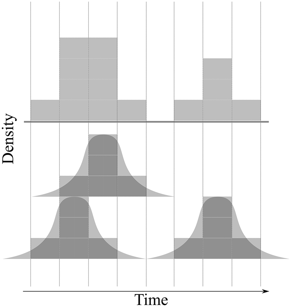
Step function summing technique developed by Geyh (1969) . Each radiocarbon-date density (represented by smooth Gaussian distributions in this image) is first approximated by a step function (represented here by blocks). Then, the height of each step function is summed for each interval of time to produce the summed radiocarbon-date curve, which is represented in this image by the blocky histogram-like figure above the double-line.
Independently, it seems, a similar notion occurred to archaeologists in the early 1970s. Rather than summing step-functions, though, early attempts to count radiocarbon-dated events involved binning median dates into temporal frequency histograms. Janette Deacon (1974), for example, used such a histogram as a proxy for fluctuations in human population levels in South Africa over the last 20,000 years. Deacon collected a database of 200 radiocarbon dates from South African archaeological sites and binned them into 1000-year time bins. The resulting distribution appeared to be dramatically increasing toward the present, which she argued indicated that population levels had increased over that period. Her reasoning was based on the idea that more radiocarbon dated sites in a given time/place indicated more people were present in that time/place. Other studies employed a similar approach with variations in sample size and temporal resolution (bin width) (e.g. Wendland and Bryson, 1974).
A few years later, in 1977, Garry Law suggested a methodological improvement (Black and Green, 1977). In a short contribution to a paper by Black and Green (1977) reporting radiocarbon sample data from the Solomon Islands, Law argued that binning median dates into a histogram failed to account for the probabilistic nature of radiocarbon assays. He proposed instead that the dates should be treated like probability densities and then added together. The approach was coincidentally similar to Geyh’s, but involved a much higher temporal resolution and, consequently, produced smoother curves.
In the following decade, proxies based on radiocarbon dates appeared in several studies that would catalyze growth in the method’s popularity among archaeologists. Michael Berry (1982) examined the temporal distribution of radiocarbon dates from the southwestern US to infer Ancestral Puebloan (Anasazi) population history from roughly 2200 to 1300 years BP. He argued that changes through time in numbers of dates from known sites tracked changes in population size and territorial abandonment. Declines in numbers of dates, he argued, corresponded to important climatic shifts in the region. Similar research involving the same logic was carried out at the same time by Gary Wright (1982) in an analysis of the population history of the Northwestern Plains of North America. Then, John Rick (1987) published a highly influential article titled “Dates as Data: An Examination of the Peruvian Preceramic Radiocarbon Record”. Using a binned-dates approach, Rick argued that radiocarbon dates from Peru indicated important spatio-temporal population dynamics including changes in landscape use and settlement distributions throughout the pre-ceramic period (roughly 20,000 to 3000 years ago). Importantly, Rick dedicated much of the paper to defending the notion of using radiocarbon dates as a proxy for population dynamics, spelling out potential biases and attempting to clarify the inferential logic behind the approach. The paper has since been cited hundreds of times and its title, “Dates as Data,” is now a common label for the approach itself among archaeologists.
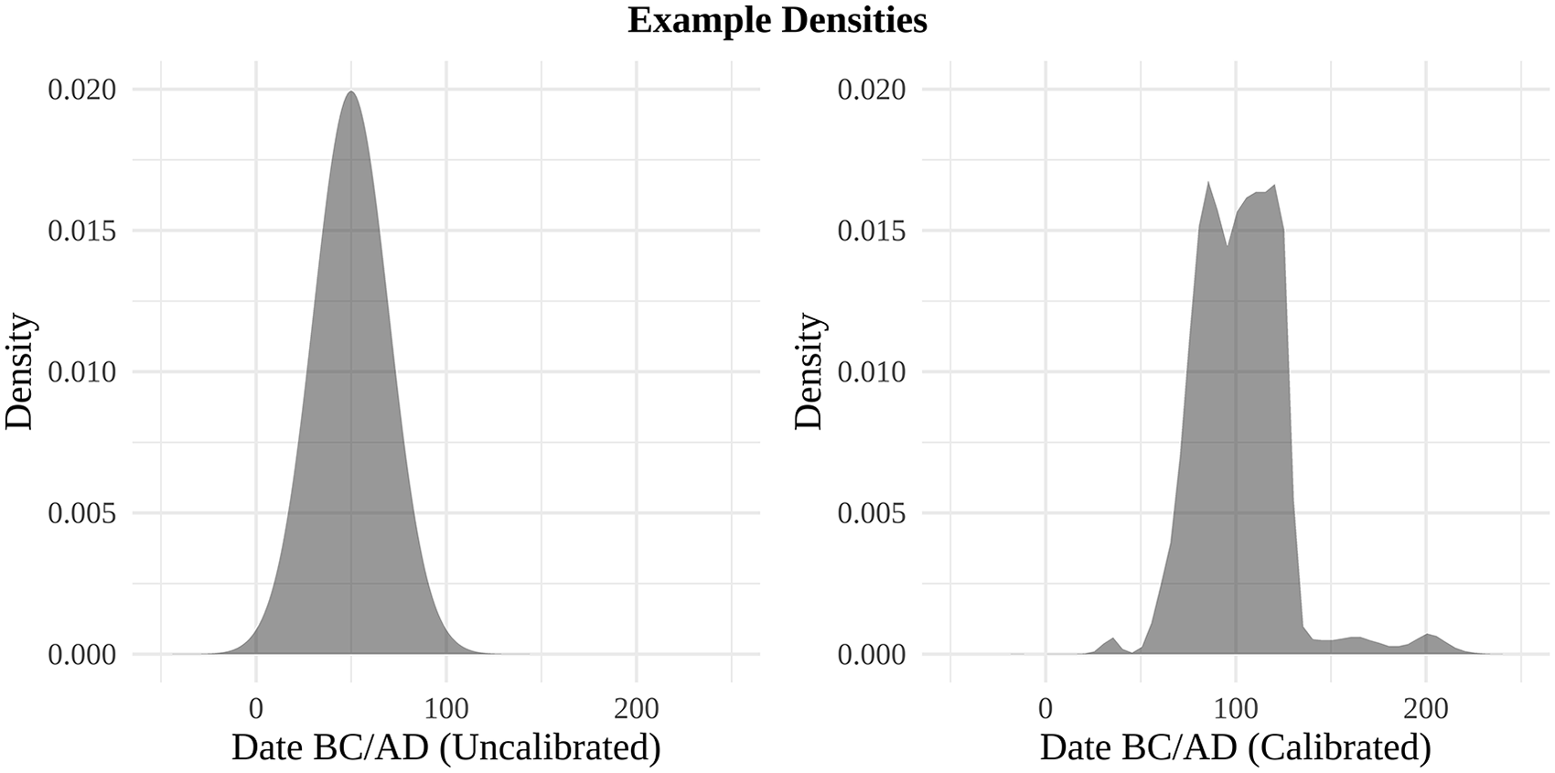
A key methodological development then occurred in the early 1990s. Up to this point, the methods for counting or summing radiocarbon-date densities involved uncalibrated dates. As Dye and Komori (1992) explained, however, aggregating only uncalibrated dates is a problem because it ignores the fact that environmental ratios of radiocarbon isotopes fluctuate through time. This fluctuation gives rise to the need to calibrate radiocarbon dates, which projects the date distribution from the radiocarbon timescale onto the calendar timescale (Taylor et al., 2014). Thus, Dye and Komori (1992) advocated applying the annual frequency distribution method developed by Law (Black and Green, 1977) to calibrated rather than uncalibrated dates. This was the first appearance of the now well-known “summed probability density function” (SPDF; see Figure 2), which is currently the most commonly-used proxy based on aggregated radiocarbon-dates.
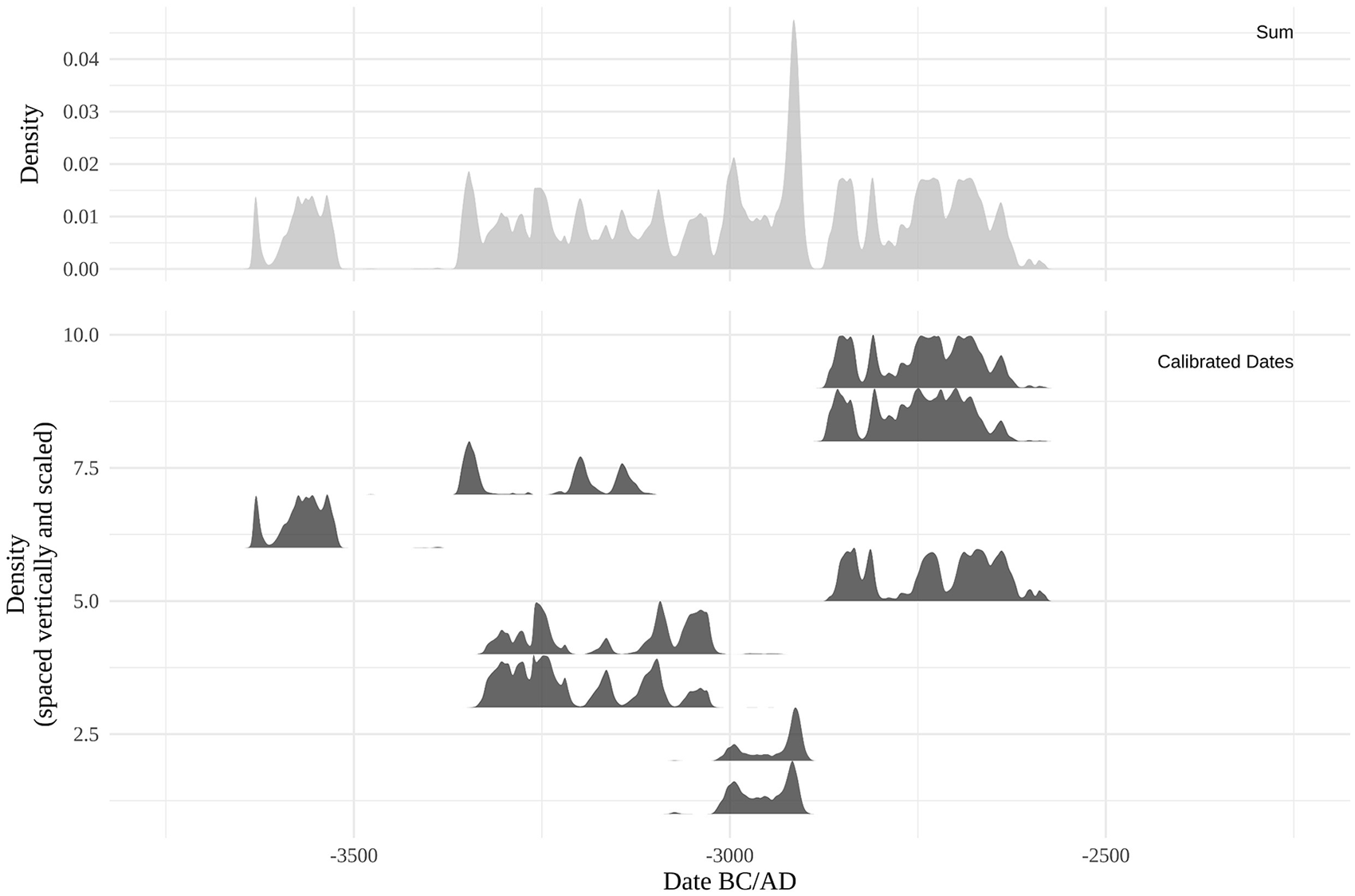
Example SPDF. Top panel (labelled “Sum”) shows an SPDF based on the individual calibrated radiocarbon-date densities in the bottom panel (labelled “Calibrated Dates”).
The proxies have become extremely popular in the last decade as relatively large databases of radiocarbon dates have become available. A Web-of-Science search for the topic “summed radiocarbon” in archaeological and interdisciplinary palaeoenvironmental science journals returned over 100 articles published since 2010 and a similar Google Scholar search returned over 400 articles. In palaeoenvironmental research the approach has been widely adopted, and the proxies have been used to study a variety of target phenomena including past sea level changes, fire-regime surges, and climatic changes more generally (e.g. Bleicher, 2013; Mooney et al., 2011; Pierce et al., 2004; Thorndycraft and Benito, 2006). Archaeologists have been particularly enthusiastic, routinely using radiocarbon dates as a proxy for past population levels (e.g. Armit et al., 2013; Collard et al., 2010; Colledge et al., 2019; Faulkner, 2011; Gamble et al., 2005; Hannah and McLaughlin, 2019; Leipe et al., 2019; Lepofsky et al., 2005; Mclaughlin et al., 2018; Prentiss et al., 2014; Schulting, 2010; Shennan, 2013; Steele, 2010; Turney and Brown, 2007).
Since their introduction in the 1970s, however, scholars have also been aware of several key sources of bias affecting the proxies (e.g. Armit et al., 2013; Bamforth and Grund, 2012; Bleicher, 2013; Brown, 2015; Contreras and Meadows, 2014; Crema et al., 2017; Deacon, 1974; Kerr and McCormick, 2014; Manning and Timpson, 2014; Rick, 1987; Williams, 2012). These include radiocarbon sample quality (Brown, 2015), the relationship between a given sample and its sedimentary context (Geyh, 1969, 1971), spatio-temporal sampling sufficiency (Crema et al., 2017; Deacon, 1974; Rick, 1987; Williams, 2012), taphonomic processes (Brown, 2015; Surovell and Brantingham, 2007; Williams, 2012), calibration artifacts (Bamforth and Grund, 2012; Brown, 2015; Geyh, 1980; Kerr and McCormick, 2014), and – in the case of archaeological research – cultural, technological, and economic effects (Rick, 1987).
The widespread recognition of these biases has led to a number of methodological recommendations (see Crema et al., 2017; Williams, 2012, for more detailed reviews). To address issues of sample quality, several scholars have advocated carefully selecting radiocarbon dates based on the perceived reliability of the dates, quality of the dated material, and consideration of depositional context – together referred to as “chronometric hygiene” (e.g. Collard et al., 2010; Ebert et al., 2017; Hoggarth et al., 2016; Shennan, 2013). To overcome sampling issues, most scholars argue that large databases of dates are required (e.g. Shennan, 2013; Williams, 2012), although little agreement exists regarding what constitutes a good sample size in this setting. And, with respect to taphonomic bias, Surovell et al. (2009) suggested that independently dated tephra-based proxies for taphonomic loss could be used to correct the preservation bias in the proxies.
In addition, there have also been recent methodological advances concerning the proxies. These improvements can be divided into two groups. One focuses primarily on null hypothesis testing – comparing an empirical SPDF to one that acts as a benchmark for determining whether the empirical SPDF differs in a statistically significant way. For the approaches in this group, observed data are either compared to SPDFs of dates simulated from theoretical growth models (Crema and Kobayashi, 2020; Manning and Timpson, 2014; Shennan et al., 2013; Wicks and Mithen, 2014) or to a baseline distribution derived from the observed data with a permutation procedure (Crema et al., 2016, 2017). The former attempts to separate the target process from well-known spurious features introduced by the calibration process (e.g. Manning and Timpson, 2014; Shennan et al., 2013), while the latter attempts to account for spurious patterns produced by sampling variability (variation in spatial sampling intensity, specifically) (e.g. Crema and Kobayashi, 2020). In contrast, the other group focuses on improving the way date densities are summarised. This includes methods like sample bootstrapping (McLaughlin, 2019), Bayesian Gaussian mixture models (unpublished function in BChron, an R package for Bayesian radiocarbon date calibration; http://andrewcparnell.github.io/Bchron/), composite kernel density estimation (CKDE) (Brown, 2017), and partially-Bayesian kernel density estimation (KDE) (Bronk Ramsey, 2017). The density estimation and mixture model approaches limit the impact of calibration curve features resulting in smooth estimates. They also produce uncertainty envelopes that help distinguish potentially important variation from spurious fluctuations caused by the calibration curve (Bronk Ramsey, 2017).
The KDE-based approaches are perhaps the most significant developments because they involve a change in the fundamental way radiocarbon-dates are aggregated (Bronk Ramsey, 2017; Brown, 2017). KDE is a commonly used non-parametric method for estimating the continuous probability density of a random variable given a finite set of realizations of that variable (Silverman, 1986). In the case of proxies based on aggregated radiocarbon-dates, the realizations are an observed set of dates while the desired density is the aggregate temporal distribution of those dates. The kernel is essentially a moving window that computes a weighted-sum of the number of radiocarbon-dated events that occurred in a given time. It assigns weights based on the temporal distance from the center of the kernel to the date of a given sample. The closer a given date is to the center of the kernel, the more it contributes to the level of the proxy at the corresponding time. Of course, the dates are uncertain and that uncertainty is expressed by a radiocarbon-date distribution. So, both Bronk Ramsey (2017) and Brown (2017) have suggested algorithms to incorporate that uncertainty into a KDE. These algorithms sample the individual radiocarbon date distributions producing a set of probable dates, one for each event in a given database. Then, they apply a KDE to the random sample of event dates to produce a smooth estimate of temporal event density. The resulting sample “curve” is also referred to simply as a KDE. This process of sampling and density estimation is repeated a large number times yielding a set of KDEs. These KDEs are then combined to produce a single average KDE – which we will refer to as KDEa to distinguish it. The set of individual KDEs can then be used to produce the uncertainty envelope mentioned earlier.
Proxies based on aggregate radiocarbon-dates have been used so far in at least two distinct ways. The first way we call the “integral approach.” Researchers employing this approach have used the proxies as approximately indicative of the total temporal distribution of events and their corresponding temporal uncertainties in a given database (Bronk Ramsey, 2017). Peaks or rises in the SPDF, for instance, are thought to indicate more events during the interval of time beneath them. This approach involves looking at the area under an SPDF and observing that more/less of that area is concentrated in one interval or another within the span of all of the relevant date densities (see Figure 3). The interpretation is downward-looking and horizontally oriented, focused on intervals of the time axis. In a sense, this view is analogous to the interpretation of an individual radiocarbon date density – that is, the probability that a given event dates to a given interval is proportional to the area under the density that spans the interval in question. In aggregate, then, more events are likely dated to periods over which the sum of many date densities has a larger area than the same sum over other periods.
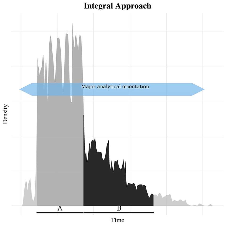
This graphic represents the “integral approach” with a simulated SPDF. Areas under the proxy are compared and interpreted like a probability density function. In this example, area A contains roughly 68% of the total area enclosed by the proxy, so it could be said that most of the total chronological information in the dataset – including uncertainty – is contained in area A, which is defined in part by a corresponding interval of time. Since it is larger than area B, one could argue that given the uncertainties in the underlying event times, most of the events have a higher likelihood of having occurred in interval A. The primary concern under the integral approach is the total temporal distribution of chronological information in the underlying dataset – that is, the distribution of dates for the events in question. The major analytical orientation, therefore, is horizontal, concerning the time-axis.
A prominent example of the integral approach is a study by Shennan (2009) of population dynamics surrounding the appearance of the Linearbandkeramik (LBK) cultural phenomenon of Neolithic Western Europe. Shennan (2009) pointed to a set of SPDFs and claimed that “[l]ow Mesolithic population levels are succeeded by a massively increased LBK population.” (p. 343) This claim appears to have been based on an integral interpretation of the relevant SPDF plots. The area under the SPDFs in those plots was much smaller in the interval before than after the accepted date for the onset of the LBK phenomenon. Thus, more of the dates – including their uncertainties – were located in the interval of time following the onset of the LBK. It follows that the events in question are more likely to be dated to the LBK period than before it. This pattern in turn, according to Shennan, indicates population levels must have increased dramatically after the onset of the LBK. The integral approach has been used extensively in numerous case studies (e.g. Becerra-Valdivia and Higham, 2020; Bishop, 2015; Boulanger and Lyman, 2013; Faulkner, 2011; Kerr et al., 2009; Lepofsky et al., 2005; Riede, 2008; Thorndycraft and Benito, 2006; Weninger et al., 2006).
We refer to the other way the proxies have been used as “point-wise” (or point-wise-like). This approach changes the orientation of analysis from the temporal distribution of events and their uncertainties (horizontal-looking) to through-time fluctuations in a given proxy (vertical-looking). It is a change from viewing the proxies as distributions of chronological information (Bronk Ramsey, 2017) to viewing them as if they are indicators of some process that may have changed through time (see Figure 4). The treatment of an SPDF/KDEa is necessarily point-wise whenever the level of the proxy at a given point in time needs to be compared to either its level at another time or another proxy at the same point in time. The proxy at time
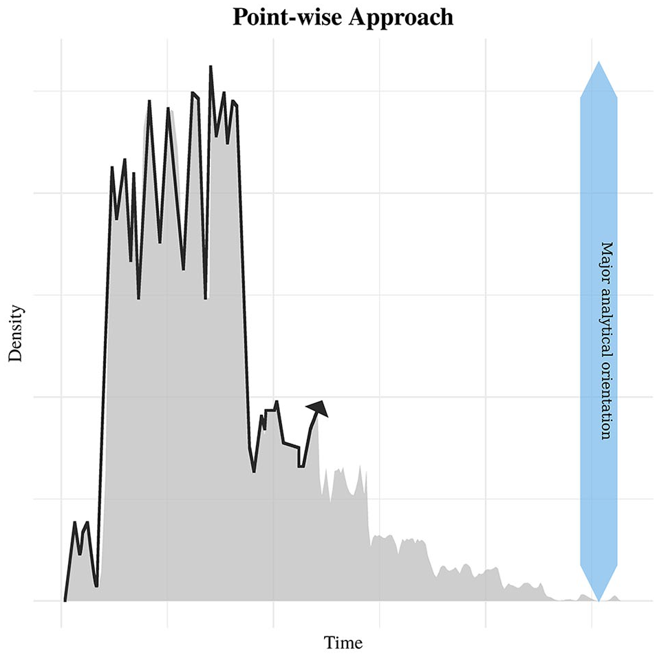
This graphic represents the “point-wise approach” with a simulated SPDF. Every point in the proxy is considered an observation that is indicative of the target process in some meaningful sense. This is required in order to estimate rates of change (i.e. compare the proxy to the passage of time itself) or to compare the proxy to other variables, like palaeoclimate reconstructions. The major analytical orientation, therefore, is vertical, concerning the measurement axis. That axis (the y-axis) is treated as if it measures the number of events dated to a particular time.
A recent example of point-wise comparisons is a paper on Late Quaternary Megafauna extinctions in North America by Broughton and Weitzel (2018). In that paper, the authors used linear regression to compare SPDFs representing megafauna populations to SPDFs representing human populations. By definition, the level of the megafauna population proxy at a given time was being mapped onto the level of the human population proxy at the same time. The average relationship between the pairings for every time under investigation was then represented by the estimated regression model parameters. The authors found a relationship between increasing human populations and declining megafauna populations for some species of megafauna between 15,000 BP and 10,000 BP. Quantitative point-wise comparisons like this occurred sporadically early on in the development of proxies based on aggregated radiocarbon-dates (e.g. Wendland and Bryson, 1974) and are becoming increasingly common (e.g. Bettinger, 2016; Ebert et al., 2017; Edinborough et al., 2017; Hannah and McLaughlin, 2019; Hinz et al., 2012; Plunkett et al., 2013; Robinson et al., 2019; Smith et al., 2008; Wang et al., 2014; Zahid et al., 2016).
Point-wise comparisons are important for understanding past processes, but it is not clear that they make sense where SPDF/KDEa proxies are involved. Ideally, point-wise comparisons would allow us to estimate rates of change in target processes and to identify potentially important casual forces by comparing a given proxy to the passage of time or to other proxy records, as we explained. Unfortunately, though, there is a good reason to think these comparisons may be unwise. Individual radiocarbon-date densities do not represent duration or through-time variation in a process that produces radiocarbon samples – they represent chronological uncertainty. It follows, then, that sums or aggregates of individual date densities also reflect chronological uncertainty in some way. Currently, to our knowledge, no attempts have been made to derive accurate point-wise interpretations for the established proxies, which leaves open crucial questions about how chronological uncertainty affects point-wise comparisons.
Here we attempt to rectify this situation. We first describe an attempt to derive interpretations for the SPDF and KDEa proxies and then we explore the downstream implications of those interpretations for point-wise comparisons. Lastly, we provide suggestions for future research that we think could improve dates-as-data approaches.
Interpreting proxies based on aggregated radiocarbon dates
For context, we imagined a hypothetical research scenario in which a large database of radiocarbon dates had been amassed. We further supposed that the individual dates represented a climatic or archaeological process. We also imagined that there was no need for a complex Bayesian calibration model because the individual radiocarbon dates were not related stratigraphically, and we assumed a good representative sample. Lastly, we assumed that each event (e.g. archaeological or palaeoenvironmental deposit) was dated by precisely one radiocarbon date density – this meant that each event was dated by only one radiocarbon sample or that a given event was dated by a pooled density of multiple samples. These simplifications aided only in the exploration of the simplest kinds of SPDF/KDEa and more complex scenarios could be considered in the same manner.
SPDF
First, we explored the SPDF. Let
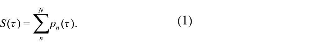
That

Since the terms in the sum are proportional to probabilities, the sum is a quantity proportional to the sum of the individual probabilities. We can, therefore, treat them as equivalent to probabilities and look to modern probability theory for the correct interpretation of
Example radiocarbon date densities. These densities represent an uncalibrated radiocarbon date of 1900 BP (50 CE) with an error of
Given standard probability theory, there are two potential interpretations of
For the first interpretation, we assume that the events are mutually exclusive, meaning that they cannot co-occur. Consider, for example, events

With respect to a pair of radiocarbon dates, mutual exclusivity would mean that the two events in question could not have happened in the same interval. Or, more formally, given two events,

where
Substituting into equation (3) two mutually exclusive radiocarbon-dated events –

The interpretation in this case is straightforward. It is the probability that at least one of the individual events occurred (Blitzstein and Hwang, 2015). In archaeological terms, it would be the probability that at least one of our imaginary radiocarbon-dated domestic buildings dates to a given time. This is essentially the interpretation described in the reference manual for OxCal under the “sum function” entry (https://c14.arch.ox.ac.uk/oxcalhelp/hlp_commands.html, accessed 2019-11-01).
If, however, the individual events are not mutually exclusive, the probability of the union must be calculated differently and this yields the second interpretation for

where the last term –
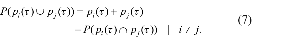
Thus, considering

it is clear that

As a result, when the events in a given sample are not mutually exclusive, the level of an SPDF,
The SPDF at any specific time conflates the number of events in a given database with uncertainty about their temporal positions. Even accounting for the probabilistic relationships among events – say by including the intersection term in equation (6) – the SPDF still refers to uncertainty. Its level at any given time indicates only the probability that at least one event occurred at the relevant time. Importantly, even the probability being indicated – at least one event – bears no necessary connection to the number of events that occurred. A few events with a high probability of occurrence at a given time would produce an SPDF value indistinguishable from a larger number of events that each had a low probability of having occurred at that time. Thus, variation from one time to the next in the level of the SPDF indicates only a change in relative probabilities, not a change in the number of events. There need not be any change in the number of underlying events for there to be fluctuations in level of an SPDF – and this would be true even in the absence of calibration artifacts or other biases.
Average KDE models
The KDEa models recently proposed by Bronk Ramsey (2017) and Brown (2017) are constructed in a very different way than a standard SPDF. Rather than summing radiocarbon-date densities at a given temporal resolution, the KDEa models are based on estimating the temporal density of radiocarbon samples. As a result, a KDEa model has a different interpretation than an SPDF. For our investigation, we primarily followed Bronk Ramsey’s (2017) definitions and approach, but the same basic process underlies Brown’s (2017) model.
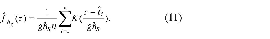
Kernel density estimation is a method for approximating an unobservable continuous distribution from a finite observed sample (Silverman, 1986). In the context of KDEa models, the samples are a database of radiocarbon dates and the continuous distribution refers to the distribution of the relevant events in time. If there was no chronological uncertainty, the continuous density at any given time,
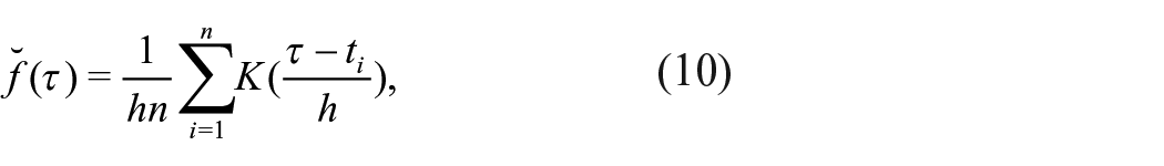
where
In order to account for chronological uncertainty in the temporal locations of radiocarbon-dated events, the KDEa approaches involve a simulation. Essentially, the simulation has three main steps. First, a sample of potential dates,
Then, a bandwidth is determined. For Bronk Ramsey’s approach, a modifier,
where
Brown’s (2017) approach differs only in that it does not involve a Bayesian treatment of the bandwidth parameter. Instead, it uses a “plug-in” bandwidth that is determined by solving a separate equation (Jones et al., 1996) for every randomly drawn set of probable event dates. Ultimately, though, it also produces an average (composite) KDEa model and an ensemble based on randomly sampled dates from the set of densities.
We discovered a precise interpretation of both KDEa models by looking at the way they account for chronological uncertainty. As we explained, each iteration of the simulation used to produce a KDEa model involves randomly drawing a set of probable dates for a given set of radiocarbon samples. So, we let
Viewing this equation, it became clear that variation at
Importantly, the second part of this interpretation means that a KDEa model does not solely reflect through-time changes in the number of radiocarbon samples – it reflects chronological uncertainty as well. Just like the SPDF, changes in the level of the proxy are also a function of chronological uncertainty, not simply the number of radiocarbon samples dated to a particular time. This mixture of through-time variation in the number of dated events and chronological uncertainty is partly what makes the KDEa useful as a summary of chronological information for a large database of radiocarbon dates. It also, however, raises problems for interpreting specific fluctuations (point-wise differences) in the model. Ups and downs in the level of the curve cannot be directly interpreted as fluctuations in the number of events dated to a given time, nor the temporal density of events at a given time. The fluctuations also represent uncertainty about the temporal locations of the events in question, specifically uncertainty about the temporal distance between them. Consequently, point-wise fluctuations in the model cannot be straightforwardly interpreted as directly indicative of through-time fluctuations in the number of events or the corresponding target process. As Bronk Ramsey (2017) explained, the KDEa approach “. . . can be used to
Discussion
Our investigation revealed a major underappreciated problem with proxies based on aggregated radiocarbon-dates: they do not represent the processes they are often thought to represent in a point-wise sense. It is important to stress that the problem does not extend to the method of radiocarbon dating more generally, only the use of aggregated/summed date densities as proxies for event counts. Both SPDF and KDEa proxies conflate chronological uncertainty with through-time variation in their target process. Neither, therefore, should be expected to clearly reflect through-time (point-wise) changes in any phenomenon related to the number of radiocarbon samples in palaeoenvironmental or archaeological records.
The conflation gives rise to several problems for point-wise analyses. We will explore the ones we think are the most obvious and important. Then, we will consider some of the main implications of these problems. Lastly, we will share some ideas for future research directions that we think could overcome them.
Analytical problems for point-wise approaches
Conceptual and statistical model mis-specification
Chiefly, the logic underpinning point-wise comparisons fails to hold because these proxies do not sufficiently indicate their intended target. This means that conceptual or quantitative models based on point-wise comparisons are mis-specified. Consequently, models involving these proxies are almost certain to be misleading. While this is a problem for both quantitative and qualitative (visual) assessments, it is easiest to understand why the problem exists in quantitative terms.
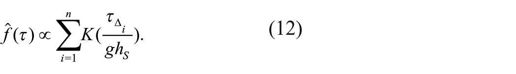
Quantitatively, a point-wise comparison makes an explicit claim about how variables might be related. One variable, often called the “response” variable, is said to be a function of one or more other variables, often called “covariates” (Rencher and Schaalje, 2008). Referring back to Figure 4, the radiocarbon proxy would be the response variable and the covariate would be the date corresponding to a given proxy measurement. This type of point-wise relationship can be expressed by a simple equation. Imagine a single response variable, say an SPDF thought to represent the number of hearths dated to a given time. Also imagine a single covariate, say a palaeoclimate proxy for temperature, that we hypothesize might be related to hearth numbers. A simple equation describing the relationship between these variables could be written as,

In this equation

But, when an SPDF or KDEa model is used as a proxy for the response, the equation would actually look more like the following (with some abuse of notation for simplicity),
The revised model is saying that temperature determines the mean of some variable that is both the number of hearths and uncertainty about whether the hearths date to the relevant time. Information about dating uncertainty is being treated in the model as if it were information about hearth-count. We cannot tell the difference between an increase in hearth count and an increase in the relative likelihood that at least one hearth is dated to the relevant time. Consequently, the model cannot be used to say anything exclusively about hearth-count.
This conflation diminishes the model’s utility as an explanation for through-time changes in the number of hearths. With the SPDF/KDEa proxies, it is as if someone poured two bags of marbles into a new bag, handed it to you, and then asked you to tell them how much each of the original bags weighed. Without more information you could never know. We cannot weigh the effect of temperature on mean hearth-count separate from its relationship to dating uncertainty. The marbles are all in the same bag.
This type of information misplacement is a kind of model mis-specification (Dennis et al., 2019; Rencher and Schaalje, 2008). The mathematical model is saying the wrong thing about the focal process. We want the model to tell us how temperature is related to the average number of hearths, but it is clearly telling us something else. Mis-specifications are known to produce biased and misleading results (Dennis et al., 2019), and the one we are describing here would have a similar effect. In fact, a recent simulation study by Brown (2017) demonstrated as much. Brown estimated a simple linear model that used a simulated SPDF as the response variable and found that the estimated regression coefficient –
The mis-specification should trigger concern for a couple of reasons. One involves the biased estimates and misleading patterns we just discussed. It makes it much harder to meaningfully compare SPDF/KDEa proxies to other variables or to make comparisons involving the same proxy at different times. This problem precludes certain lines of research altogether – like identifying rates of change, or distinguishing the impacts of one potential causal factor from another.
The other reason is more grave. While some scholars may choose to see biases affecting statistical models as merely a technical nuisance, the main reason for concern is that the point-wise comparisons necessary for creating such a model make no scientific sense. These proxies mix up chronological uncertainty with their intended target in such a way that the two values cannot be unmixed. So, even if a covariate looks as if it may explain variation in the target process, what is actually being explained will always be a combination of variation in chronological uncertainty
Strange non-independence
A second, closely related, analytical problem involves observation independence. For both the SPDF and KDEa model, neighbouring observations have an unusual effect on each other. If one observation is proposed to be true – that is, accurately reflects the underlying number of events at a given time – the neighbouring observations
To illustrate, consider a single calibrated radiocarbon-date density. Variations in the level of the density indicate the relative probability that the event in question occurred at a given time. If it did occur in a particular time, however, it cannot have occurred in another time. The same logic applies to the SPDF and KDEa models. If we imagine for a moment that the level of an SPDF at time
This inter-temporal dependence has two immediately obvious consequences. One is that the error terms in a typical regression model are no longer independent. Referring back to the examples above (equations (13)–(15)), the dependence means that the
The other consequence of the unusually complex inter-temporal dependence in SPDF/KDEa proxies is that the proxies cannot be mapped to covariate observations in a stable, consistent way. It is impossible to determine whether a given proxy observation – say the level of an SPDF at time
Finite observations and infinite sample sizes
A third problem is that these proxies can give a false impression of the number of observations available with consequences for the identification of significant features/findings. In a classical statistical setting, “significance” often depends on the number of unique and independent pieces of information contributing to a perceived pattern. This is why standard text books devote space to discussing the importance of sample size (e.g. Devore, 2012; Ryan, 2013). Far from being unique to statistical applications, though, it is simply good scientific practice to be aware of how many observations are required to be confident that an identified pattern reflects reality.
The aggregate proxies, however, can be sampled at an arbitrarily high rate. This allows for a kind of quantitative alchemy whereby a finite number of individual radiocarbon-dated events can be transmuted into a sample of unlimited size. An individual radiocarbon-date density, for instance, is an approximation of an underlying function that can be produced at any resolution. Often the default for calibration programs is 5 or 10 years, but there is no hard cap in theory with the only limiting factor being a trade-off between spuriously high precision and accuracy. So, an SPDF or KDEa model could, for example, be annually resolved and span millennia. This would result in an apparent sample size in the multiple thousands, even if the SPDF was ultimately based on only a dozen dates.
A statistical model, unfortunately, could not “know” the difference – they are just equations, after all, and it is up to the one using them to decide whether they apply in a given case. Most common approaches (regressions or time-series methods, for example) entail counting the number of observations in the SPDF in order to determine sample size. This would mean that the sample size was the number of time-points at which the proxy was sampled, which is determined by its resolution, not the number of dates used to create the proxy in the first place. Scientifically, though, it is the number of dates that indicate how many unique pieces of information are involved in the analysis, at least with respect to models seeking to explain event count variation.
For point-wise comparisons, we think this sample size problem is unavoidable. While several archaeologists have cautioned that sample sizes need to be large for SPDFs/KDEas to be meaningful (e.g. Bishop, 2015; Contreras and Meadows, 2014; Williams, 2012), it is nonetheless always possible to oversample these models. Thus, these proxies will tend to give the impression that the sample size is much larger than it actually is. More importantly, there is no obvious relationship between the number of dates used to create a proxy and the appropriate sampling rate that should be used in order to avoid oversampling. Ultimately, the problem again stems from confusing chronological uncertainty with event counts. Single date densities, representing only one sample, are treated like representations of through-time processes when they are aggregated with the densities of other samples. Individually, the densities do reflect some latent, smooth process that has to do with radiocarbon-dating uncertainties (e.g. isotope instrumentation error, calibration curve uncertainties, through-time fluctuations in environmental carbon isotope ratios, etc.). But aggregated together and used as a proxy for a radiocarbon sample producing process, the smooth line is thought to reflect event-count. In the former case, one could justifiably assume that there is some smooth underlying process represented by a date density and then sample it at whatever rate was reasonable – this is the basis for Functional Data Analysis where a smooth estimate based on a finite sample actually does represent an underlying continuous process (Ramsay et al., 2009). With proxies based on aggregated radiocarbon-dates this is simply not the case. At least, the continuous underlying process that could be sampled is a reflection of chronological uncertainty, not through-time changes in the number of events. It is the latter most scholars are interested in and the way that the established proxies are often interpreted.
Misleading density-like structure
The last major analytical problem is that chronological uncertainty imposes a characteristic structure on these proxies that can be misleading. Chronological uncertainty is inherently density-like, by which we mean shaped like a density function (e.g. a bell-curve). Uncertainty about the timing of an event means that we assign some likelihood to the event having occurred at a given time and that likelihood declines with increasing temporal distance from that most likely time. As one might expect, this density-like structure applies to individual radiocarbon-date densities, sums of radiocarbon-date densities, and of course KDEas based on radiocarbon-date densities.
A density-like structure creates a confounding problem for point-wise approaches. Any density function has to have a positive finite integral – that is, the area between a continuous density function (curve) and its domain (x-axis) has to be entirely above the domain (positive everywhere) and it has to have a finite limit (the area cannot be infinitely large) (Blitzstein and Hwang, 2015). In more concrete terms, our uncertainty about the timing of one or more events is not infinite, so a curve representing that uncertainty must occupy a finite amount of time. This means that the curve can go up and down in any manner, but it must “begin” by going up and “end” at some point by going down. The same is true of aggregated density functions representing groups of individual events, like the SPDF and KDEa. Sometimes, a given proxy may exhibit several up/down fluctuations, but overall the up-then-down pattern will be consistent irrespective of the true through-time structure of the target process. Consequently, whatever the true relationship looks like for a given process–covariate pair, the relationship between a corresponding proxy and the covariate will be distorted. Ultimately, the distortion occurs because we are uncertain about the timing of the individual events in question and our uncertainty has a natural density-like structure. Importantly, this structure cannot be accounted for separately from variation in event-count when SPDF/KDEa models are used.
Implications
The problems we identified can lead scientists severely astray in point-wise analyses. Determining the magnitude of the problem depends on many factors that will be particular to a given dataset and analysis. These include the number of dates involved, the span of time under analysis, the level of calibration curve uncertainty, the slope of the calibration curve, and the variation in the target process. These factors will affect the “signal-to-noise” ratio – that is, the magnitude of variation in the target process relative to the level of chronological uncertainty. If, for example, the underlying target process changes dramatically over a given interval of interest, then certain features of an SPDF/KDEa proxy of that process may be vaguely representative assuming (1) a high enough sampling rate (number of dates per unit of time) and (2) low chronological uncertainty per date relative to the length of interval of interest. But, the chronological uncertainty will be present nonetheless and the problems we described above will continue to hinder attempts to recover underlying patterns. Importantly, the problem of inter-temporal dependence will still be present, and the overall density-like structure of the proxy will distort the true target process. Thus, faulty inferences are very likely, even when attempting to address an elementary research question like whether a given target process increased, decreased, or remained constant through time.
To demonstrate, we conducted a simple simulation. The target process in our simulation was a simple uniform function – meaning, no change through time and an average slope of zero. It would be analogous to, say, population levels that were constant through time. We then used standard regression models to try and estimate the slope value. The goal was to determine whether false-positive findings were likely and, if they were, to figure out whether the conflation between chronological uncertainty and process variation was likely to blame.
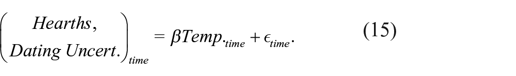
First, we created a uniform process over a 1000-year interval with a start date chosen at random from between 48,000 and 2000 BP (see Figure 6). We then sampled the uniform process randomly, drawing 1000 event-dates from it. Next, we used the “calBP.14C” function from the R package, “clam” (Blaauw, 2020), to derive uncalibrated dates from the event-date sample, which we subsequently calibrated with the “calibrate” function from the same package. We then created three time-series. One was an SPDF based on the simulated calibrated dates. The second was a count time series of the event-date sample – this series represents a high-fidelity sample of the true process with no chronological error. The last was a density estimate of the event-date sample, produced with R’s built-in “density()” function. This series was approximately like an SPDF/KDEa model, but without any chronological error. It allowed us to isolate the distorting effects that smooth density estimates would be expected to have on regression models from the specific effect of conflating chronological uncertainty with process variation as the SPDF/KDEa proxies do.
Simulated SPDF data. The bottom time series represents the target uniform process. The center series represents the count series corresponding to the random event-date sample of 1000 observations. The top series is the corresponding SPDF proxy.
With these data in hand, we ran three regressions using R’s “glm()” function. In one, we used a Gamma-distributed model with the simulated SPDF as the response variable and time as the only covariate. For the second one we used the count-series as the response variable and time as the covariate in a Poisson model. For the last regression we produced another Gamma-distributed model with the chronological-error-free density estimate as the response variable.
The regression results were very clear. Unsurprisingly, the models involving the chronological-error-free time-series indicated that the slope of the target process was indistinguishable from zero (see Figure 7). The SPDF regression, however, produced a very different result. The target estimate was severely biased, with the mean very far from zero (see Figure 7). Crucially, it also indicated that the non-zero effect was highly statistically significant, well beyond the standard 95% or 99% confidence levels. We re-ran this simulation repeatedly with consistent results. Using an SPDF in a point-wise analysis can be very misleading for the reasons we outlined. The simulation described in our SI demonstrates similar problems for the KDEa proxy.
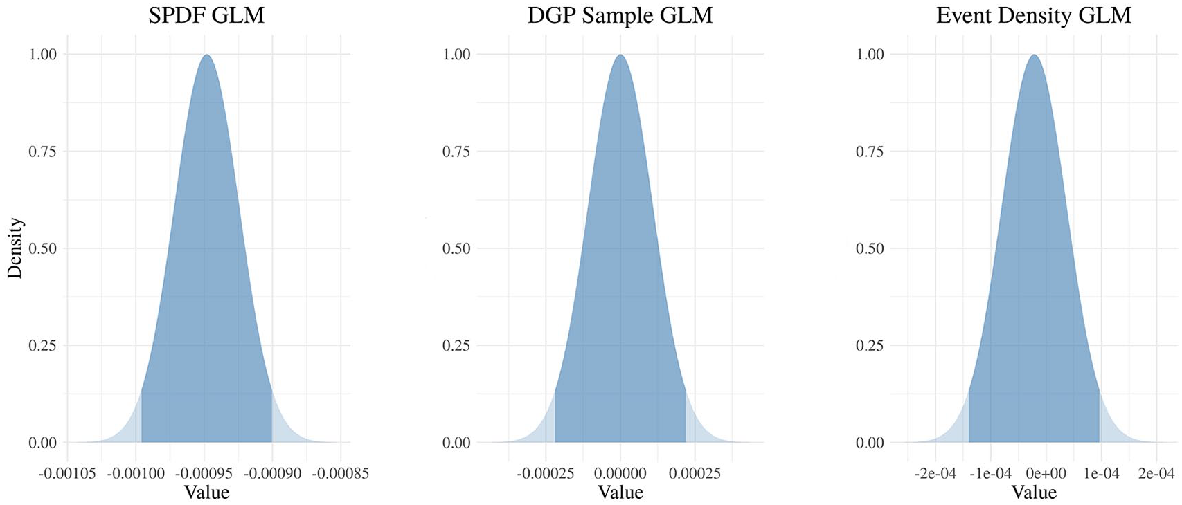
Regression simulation parameter estimates. The two densities were created by using the regression coefficient parameters estimated from our two regression models. The density on the left represents the sampling distribution for the regression coefficient related to time in the SPDF regression model. The density in the center represents the sampling distribution for the corresponding coefficient in the Poisson model based on the sample of event-dates. And, the distribution on the left represents the same information for the model involving the density estimate of the event-dates. The dark blue areas indicate the 95% confidence regions and the lighter blue areas represent the 99% regions.
These problems have important implications for past and future research. A major implication for previous research is that published findings based on SPDF/KDEa proxies could be misleading. In more qualitative studies involving no regression models (e.g. Bradtmöller et al., 2012), narratives about through-time processes like demographic changes or fluctuations in sea level may be telling the wrong story. In more quantitative research involving correlation and/or regression (e.g. Bettinger, 2016), hypothesis tests could be invalid and parameter estimates false or biased, calling into question inferences drawn from such findings. In light of the potential problems we have identified, this body of research should be viewed with some measure of suspicion, in our view.
A major implication for future research is that these proxies should be avoided when point-wise interpretations are necessary or implied. They could instead be profitably used for addressing some questions about chronological relationships. Research into, for example, whether a collection of events pre- or post-dates a fixed date could also be based on the established proxies (e.g. Bronk Ramsey, 2017). This is the “integral approach” we described earlier whereby the analysis is focused on the relative sizes of areas under the proxies and the corresponding intervals of time covered. Comparing these areas does not appear to be conflating process variation and chronological uncertainty in the same manner as the “point-wise” approach does. It is important to emphasize, though, that more systematic and mathematically grounded approaches exist for estimating the relevant probabilities (Bronk Ramsey, 2009; Buck et al., 1996) and, at best, an SPDF or KDEa may only be appropriate for visualization. Research intended to improve our understanding of through-time fluctuations in the number of radiocarbon-dated events, however, should not be based on these proxies.
Directions for future work
We imagine future research proceeding in two main directions. One involves a review of previous studies. Many of the published studies involving proxies based on aggregated radiocarbon-dates should be re-evaluated to determine whether the problems we identified undermine previous conclusions. This is especially the case where interpretations depend on the point-wise approach. We recognize that determining whether a given argument or study depends on point-wise interpretations may be challenging for qualitative cases because of the vagueness of the language sometimes used. But, reports that highlight short-term fluctuations in these proxies, or reports that involve claims about rates of change or magnitude of fluctuations, should probably be considered suspect. Similarly, claims about “events,” like rapid declines in event counts, must be relying on point-wise comparisons because identifying a “rapid change” requires one to evaluate the difference between levels of a given proxy at neighbouring or nearby times. Quantitative research, in contrast, will be easier to evaluate in this regard because it is necessarily point-wise and the claims being made must have been explicitly spelled out.
The other direction for future research involves methodological development. As is hopefully clear, we think that the main problem with using dates-as-data in point-wise analyses is the confounding between chronological uncertainty and process variation. There are potentially useful alternative approaches, though. In a study on chronological uncertainty in layer-counted archives, for example, Boers et al. (2017) proposed a method of re-projecting uncertainty from the time-domain onto the measurement domain. It takes chronological uncertainty and turns it into measurement uncertainty, which would make point-wise comparisons more sensible. Rather than conflating chronological uncertainty with event counts, the reprojected proxy would ideally indicate the probable number of events that occurred in a given time. That way, point-wise conceptual or quantitative models would be explaining variation in one dimension exclusively. The method they proposed was developed for use with layer-counted archives – e.g. ice cores, or varved lake sediments – but it might be adapted for use with radiocarbon-dated events. A persistent challenge will be finding a way to correctly account for the non-independence between observations, but further research is warranted.
Another recent development involves a Bayesian regression approach for analyzing radiocarbon-dated event-count series. These Radiocarbon-dated Event Count (REC) models have been tested with simulated data and appear to be able to separate target process dynamics (event-counts) from chronological uncertainty (Carleton, 2020). REC models effectively extend the basis of the KDEa approaches (Bronk Ramsey, 2017; Brown, 2017) but are directed at regression model estimation rather than density estimation. They are based on ensembles of potential event-count sequences created by sampling the corresponding calibrated radiocarbon-date densities – a Radiocarbon Event-Count Ensemble, or RECE. Each member of the RECE is then placed in a suitable regression model. The individual models are nested in a multi-level Bayesian framework so that priors for target parameters (e.g. regression coefficients) can be specified. As such, no individual regression model conflates uncertainty with process variation – these types of information are kept separate. At the same time, chronological uncertainty is accounted for in the posterior distributions of the top-level parameters. Further methodological exploration of REC models could go some way toward making the dates-as-data paradigm viable in the context of point-wise comparisons aimed at rate estimation, model comparison, and standard hypothesis testing.
Conclusion
Proxies for radiocarbon-dated event counts are tempting to use and have appeared in hundreds of scholarly articles since their inception. They are generally intended to represent through-time fluctuations in the amount of radiocarbon in the archaeological and palaeoenvironmental records. These through-time fluctuations are thought to be caused by variation in one or more radiocarbon-producing target processes, including past human activity, population level changes, sea-level changes, and surging fire regimes. However, there are lurking problems that make these proxies unsuitable representations of their targets when viewed in a point-wise way. The main problem is that these proxies do not clearly reflect through-time variation in the number of radiocarbon-dated events in a given database. Rather, they combine through-time variation with chronological uncertainty. Unfortunately, this conflation is easy to miss, leading to biases and faulty interpretations. We, therefore, urge scholars to think carefully about how the proxies are being interpreted and whether they are appropriate for a given research agenda. Any researchers intent on using the proxies will need to explain precisely why the problems we have identified are not materially affecting their interpretations. Alternative approaches that avoid the conflation are under development and scholars interested in using radiocarbon-dates as data should consider using those methods instead.
Supplemental Material
sj-pdf-1-hol-10.1177_1049732320931430 – Supplemental material for Sum things are not what they seem: Problems with point-wise interpretations and quantitative analyses of proxies based on aggregated radiocarbon dates
Supplemental material, sj-pdf-1-hol-10.1177_1049732320931430 for Sum things are not what they seem: Problems with point-wise interpretations and quantitative analyses of proxies based on aggregated radiocarbon dates by W. Christopher Carleton and Huw S Groucutt in The Holocene
Supplemental Material
sj-pdf-2-hol-10.1177_1049732320931430 – Supplemental material for Sum things are not what they seem: Problems with point-wise interpretations and quantitative analyses of proxies based on aggregated radiocarbon dates
Supplemental material, sj-pdf-2-hol-10.1177_1049732320931430 for Sum things are not what they seem: Problems with point-wise interpretations and quantitative analyses of proxies based on aggregated radiocarbon dates by W. Christopher Carleton and Huw S Groucutt in The Holocene
Supplemental Material
sj-R-3-hol-10.1177_1049732320931430 – Supplemental material for Sum things are not what they seem: Problems with point-wise interpretations and quantitative analyses of proxies based on aggregated radiocarbon dates
Supplemental material, sj-R-3-hol-10.1177_1049732320931430 for Sum things are not what they seem: Problems with point-wise interpretations and quantitative analyses of proxies based on aggregated radiocarbon dates by W. Christopher Carleton and Huw S Groucutt in The Holocene
Footnotes
Acknowledgements
We would like to thank the editor, Professor John Matthews, and three anonymous reviewers for their helpful comments and feedback. We would also like to thank Professor Caitlin Buck for her helpful correspondence early on in the research process.
Funding
The author(s) disclosed receipt of the following financial support for the research, authorship, and/or publication of this article: Funding for this research was provided by the Max Planck Society.
Supplemental material
Supplemental material for this article is available online.
References
Supplementary Material
Please find the following supplemental material available below.
For Open Access articles published under a Creative Commons License, all supplemental material carries the same license as the article it is associated with.
For non-Open Access articles published, all supplemental material carries a non-exclusive license, and permission requests for re-use of supplemental material or any part of supplemental material shall be sent directly to the copyright owner as specified in the copyright notice associated with the article.