Sage Journals: Discover world-class research

Abstract

High-resolution paleoceanographic reconstruction of surface water properties during the most recent Sapropel event (S1) has been carried out by means of quantitative analyses of planktonic foraminiferal assemblages, planktonic foraminiferal oxygen isotopes (δ¹⁸O) and XRF elemental data from a 655 m depth core recovered in the North Ionian Sea. The results show that the S1 interval presents two distinctive warm phases (S1a and S1b), separated by a cold interruption event (S1i). High resolution faunal and geochemical analyses allow to identify two sub-phases within S1a interval, the oldest one has similar characteristics to S1b interval while the youngest sub-phase has less stratified surface waters with relatively lower nutrient content. The high abundance of Globigerinoides ruber white variety opposite to the low percentages of Neogloboquadrina pachyderma during the pre-S1 phase suggests that the onset of surface waters stratification occurred prior to the beginning of Sapropel deposition, acting as a pre-conditioning phase. Paleo-productivity proxies indicate that the deposition of S1 initiated after an increase in nutrient content, potentially related to increased fluvial inputs. Based on the integrated ecological interpretation of our records we argue that S1a and S1b are characterized as warm, stratified and nutrient rich surface waters in the Ionian Sea, while proxies related to oxygen content indicate dysoxic deep waters linked to a combination of the high nutrient content and stratified water column. The S1 interruption phase is characterized by the entrance of colder waters that caused mixing of the stratified water column and re-ventilation of the deep dysoxic waters.

Keywords

Mediterranean Sea North Ionian Sea Paleoceanography planktonic foraminifera Sapropel 1 XRF elemental ratios

Introduction

The deposition of dark-coloured, organic-rich sediment layers (Sapropels) in the eastern Mediterranean Sea have been described and characterized by several studies (Calvert et al., 2001; Casford et al., 2002, 2003; De Lange et al., 1999, 2008; Filippidi et al., 2016; Geraga et al., 2008; Giamali et al., 2019; Kallel et al., 2000; Kontakiotis, 2016; Kontakiotis et al., 2009, 2013; Kotthoff et al., 2008; Mélières et al., 1997; Plancq et al., 2015; Rohling, 1994; Rohling et al., 1997, 2015; Siani et al., 2010; Tesi et al., 2017;). However, there is a lack of consensus on the precise mechanisms and the exact sequence of climatic and oceanographic events that lead to the formation of Sapropels. It is generally accepted that Sapropels are the result of complex interactions between regional climatic, oceanographic and biogeochemical processes as a response to shifting global climate patterns (De Lange et al., 2008; Grimm et al., 2015; Le Houedec et al., 2020; Mercone et al., 2000, 2001; Rohling et al., 2015; Tachikawa et al., 2015; Vadsaria et al., 2019). Sapropel 1 (S1) is the only sapropel event that appears during Early-Mid-Holocene (interglacial period), between 10.8 ± 0.4 and 6.1 ± 0.5 kyrs BP (De Lange et al., 2008; Incarbona et al., 2019). General consensus suggests that the deposition of S1 was caused by the combination of three main factors. First, the freshening and stratification of Mediterranean surface waters, both from low salinity Atlantic inflow through Gibraltar Strait as well as from increased river runoff (Geraga et al., 2010; Kontakiotis, 2016; Kontakiotis et al., 2009, 2013; Mojtahid et al., 2019) resulting from northward shifting and intensification of the African monsoon (De Lange et al., 1999, 2008; Grant et al., 2016; Hennekam et al., 2014; Rohling, 1994; Rohling et al., 1997, 2015). Second, the increased river discharge was accompanied by a resupply of land-derived nutrients to the surface ocean, followed by enhanced primary productivity and export of organic matter to the bottom of the basin (De Lange et al., 2008; Rohling and Gieskes, 1989; Rohling et al., 1997). Third, enhanced surface ocean stratification also resulted in reduced ventilation rates of the deep waters through deep water convection (i.e. reduction in dissolved oxygen export) that in turn favoured the preservation of the organic matter due to the establishment of dysoxic conditions (Abu-Zied et al., 2008; De Lange et al., 1999, 2008; Drinia et al., 2016; Grimm et al., 2015; Le Houedec et al., 2020; Louvari et al., 2019; Rohling et al., 2015; Schmiedl et al., 2010). All these factors together could contribute to the formation of the Eastern Mediterranean (EMED) S1 layer.

Several studies have shown that S1 can be subdivided into two distinctive phases (S1a and S1b) separated by an interruption phase (Giamali et al., 2019; Kontakiotis, 2016; Myers and Rohling, 2000; Rohling et al., 1997; Rohling and Pälike, 2005; Triantaphyllou et al., 2009). While both S1a and S1b were periods of warm, stratified waters with dysoxic bottom conditions, the interruption period (S1i) was characterized by the arrival of cold surface waters, which favoured vertical mixing and enhanced re-ventilation of the EMED deep waters (De Rijk et al., 1999; Incarbona et al., 2019; Myers and Rohling, 2000; Rohling et al., 1997, 2015; Rohling and Pälike, 2005; Schmiedl et al., 2010;). The onset and the end of S1 deposition throughout the eastern Mediterranean Sea appears to not have been synchronous (10.8 ± 0.4–6.1 ± 0.5 kyrs BP; De Lange et al., 2008), independently of the water depth of deposition (De Lange et al., 2008; Klein et al., 2000; Schmiedl et al., 2010). However, although S1 has been characterized in many different locations through the Eastern Mediterranean, there is a lack of information available on the northern part of the central Mediterranean basin (Adriatic and Ionian Seas).

This study is focused on the study of the expression of S1 in the northern part of the Ionian Sea, which is a key area for understanding the Mediterranean thermohaline circulation (MedTHC) system. In this sense, the Ionian Sea acts as an important gateway between the Adriatic Sea and the rest of the Mediterranean, where water exchange occurs both at surface and intermediate-deep levels. Surface and intermediate waters from the Ionian Sea enter the Adriatic Sea forming a cyclonic gyre, while Adriatic Deep waters (ADW) overflow to the Ionian Sea (Cushman et al., 2001; Manca et al., 2003). These complex interactions between the Adriatic and the Ionian Sea make this study area a key gateway zone. With the objective of understanding the hydrographic changes that lead to the Sapropel formation in the study area, we present the first high resolution dataset with precise chronology for the North Ionian Sea, containing proxy records from planktonic foraminifera assemblages, stable isotopes (δ¹⁸O) and bulk XRF elemental composition of sediments. Although S1 has been previously defined as having two main phases (S1a and S1b), their characterization has never been done at very high resolution, thus lacking the possibility of identifying centennial or even decadal variability within this time interval. Thus, the final goal of this study is the understanding of the hydrographic changes that lead to the Sapropel S1 formation in the central Mediterranean at very high resolution (centennial or decadal) along with the reconstruction of the oceanographic conditions and climate variability over this time interval.

Study area

The Mediterranean is a semi-enclosed Sea divided by two main basins, the western and eastern Mediterranean, separated by the Sicily channel (Figure 1). Its reduced spatial scale, partial isolation and marginal configuration make the Mediterranean Sea an excellent “natural laboratory” acting as an amplifier, where climatic and oceanographic processes can be studied with a better signal to noise ratio compared to the open ocean (Antonarakou et al., 2019; Cacho et al., 2001; Kontakiotis, 2016; Rohling et al., 2015). The Mediterranean Sea sediments have proved to be an excellent archive where climatic events can be recorded (i.e. Bazzicalupo et al., 2020; Koutrouli et al., 2018; Lirer et al., 2013; Margaritelli et al., 2018). Typically, high sedimentation rates during the Holocene represent one of the most powerful tools to monitoring the climate evolution by amplifying the climatic signals over the Holocene (Antonarakou et al., 2018; Cacho et al., 2001; Giamali et al., 2019; Louvari et al., 2019; Marino et al., 2009).

Figure 1.

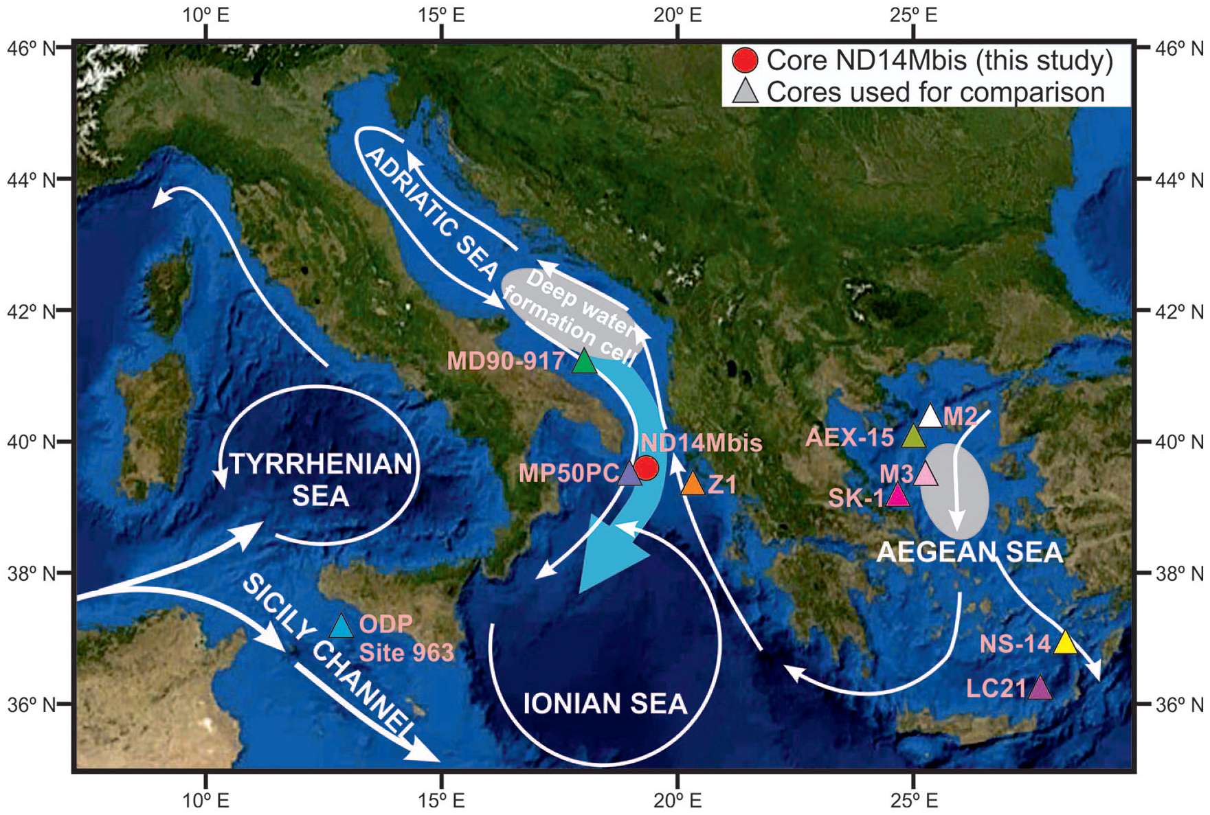
Map of the study area showing the modern surface (white arrows) and deep (blue arrow) circulation patterns based on Rohling et al. (2009), and also core ND14Mbis location. Other reference core sites used in the text for comparison (LC-21, Casford et al. (2002) and Rohling et al. (2002); ODP Site 963, Sprovieri et al. (2003); M2 and M3, Roussakis et al. (2004); Z1, Geraga et al. (2008); MD90-917, Siani et al. (2010); MP50PC, Filippidi et al. (2016) and Filippidi and De Lange (2019); SK-1 and NS-14, Kontakiotis (2016); AEX-15, Giamali et al. (2019) are also shown.

The study core ND14Mbis is located at the north-east end of the Ionian Sea. The Ionian Sea waters are connected with the Adriatic Sea on the north by the Otranto strait, with the Aegean Sea on the east and the Tyrrhenian Sea on the west through the Sicily Channel. Adriatic deep waters (ADW) typically overflow through the Otranto strait and contribute as one of the main sources and precursors of Eastern Mediterranean Deep Waters (EMDW) (Manca et al., 2003) (Figure 1). Across the Sicily Channel, a surface layer of strongly Modified Atlantic Water (MAW) enters the Levantine basin from the western Mediterranean (Figure 1). That surface water inflow is balanced out through the outflow of intermediate (Levantine Intermediate Water, LIW) and deep (EMDW) waters into the Tyrrhenian Sea (Garcia-Solsona et al., 2020; Manca et al., 2003) (Figure 1).

The Adriatic Sea typically presents lower surface salinities than the rest of the Mediterranean, mostly due to large fresh water discharge from rivers (e.g. Po River, Ofanto River), and it collects up to a third of the total annual fresh water discharge into the Mediterranean, thus acting as a dilution basin (Manca et al., 2003; Özsoy et al., 1989). In the southern part of the Adriatic Sea, there is a deep water convection cell that forms dense waters (ADW) (Cushman et al., 2001; Özsoy et al., 1989) (Figure 1). The formation of this water mass starts with the pre-conditioning of surface waters with sustained cold, dry north-easterly winds. As a result, buoyancy loss of surface waters through intense cooling and evaporation result in the establishment of a deep water convection system. The ADW is formed when this denser and cold waters flows towards the deep South Adriatic basin and mixes with LIW, a relatively warm and salty water mass. The result of this mixing is a denser water mass (the ADW) that spills over into the Ionian Sea through the Otranto strait and sinks into the deep basin becoming the primary source of EMDW (Cushman et al., 2001; Özsoy et al., 1989, Figure 1). Being a dilution basin, the Adriatic Sea exports relatively fresh surface waters to the Ionian Sea which is compensated by the inflow of warmer and saltier waters from the eastern Mediterranean through the surface and intermediate water layers (Cushman et al., 2001). The surface ocean currents flow counter-clockwise from the Strait of Otranto, passing by the eastern coast and then southward to the strait by the western (Italian) coast (Figure 1).

Material and methods

This study focuses on the S1 sedimentary sequence of the gravity core ND14Mbis, recovered during the Next-Data 2014 expedition on board of the Italian Vessel R/V Urania-CNR. The core is located at the north-eastern part of the Ionian Sea (39°35′53,94″N, 18°47′40,48″E, 655 m depth) (Figure 1) along the exit pathway of deep waters from the Adriatic Sea into the Ionian Sea. Core length is 332 cm and the studied interval is located between the interval 80–150 cm, which comprises the pre-Sapropel, the Sapropel layer (between 105 and 126 cm) and the post-Sapropel intervals. The Sapropel interval is characterized by two dark layers of 11 and 5 cm respectively, interbedded by a light interval of 5 cm, above the Sapropel unit, we can see a 2 cm light dark layer (between 103 and 105 cm) lithologically similar to the sapropel (Figure 2a). For this study, the entire core was sampled at 1 cm resolution.

Figure 2.

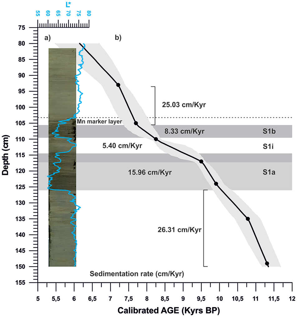
(a) High resolution digital image of core ND14Mbis and lightness values (L*) (blue line) acquired with the high-resolution colour line scan camera of Avaatech XRF core scanner at the CORELAB laboratory of the University of Barcelona. Different phases within sapropel 1 are identified with black boxes (S1a, S1i and S1b) and the Mn marker layer has been highlighted with a dotted line. (b) Age model of core ND14Mbis around Sapropel 1 time interval (marked in grey). Age-depth correspondence is marked with a white line while the light grey cloud represents age uncertainties (2 sigma). Corresponding sediment accumulation rates are also shown.

Stable isotopes

We have measured oxygen stable isotopes (δ¹⁸O) on Globigerinoides ruber white variety, through S1 interval at 1 cm resolution (71 samples). Between 10 and 15 specimens of G. ruber white (>150 µm) were picked. The samples were crushed and sonicated in methanol to remove fine-grained detrital particles. These analyses were performed with a mass spectrometer Finnigan MAT 252 fitted with a carbonate preparation line (Kiel device), at the University of Barcelona (CCiT-UB). The estimated external reproducibility is typically <0.05‰ for δ¹⁸O. Calibration to Vienna Pee Dee Belemnite (VPDB) was carried out following NBS-19 standards (Coplen, 1996).

X-ray fluorescence (XRF)

Bulk elemental geochemical composition of core ND14Mbis was measured with an Avaatech XRF core scanner at the CORELAB laboratory of the University of Barcelona. The sediment core was measured at 1 cm resolution with excitation conditions of 10 kV, 0.5 mA and 10 s for major elements (Al, Si, S, K, Ca, Ti, Mn, Fe), 30 kV, 1.0 mA, 30 s with a Pd-thick filter for Br, Rb, Sr and Zr, and 50 kV, 1.0 mA, 30 s and a Cu filter for Ba. In addition, the core section corresponding to S1 interval (dark layers in Figure 2a) was measured at 2 mm resolution with excitation conditions of 10 kV, 1.0 mA and 10 s, 30 kV, 1.4 mA, 45 s with a Pd-thick filter, and 50 kV, 1.4 mA, 45 s and a Cu filter. The relative abundance of the elements of interest is shown as elemental ratios normalized to Al as a way to avoid the dilution effect that happens to some elements (Calvert and Pedersen, 2007).

Planktonic foraminiferal assemblages

The planktonic foraminiferal analysis was realized on a total of 71 samples with 1 cm resolution. The bulk sediment samples were dried at 60°C in the oven and then wet sieved through a 63 µm mesh to separate sand and clay fractions. Quantitative planktonic foraminiferal analysis was done in the >150 µm fraction. For each sample a number between 200 and 300 individuals were counted and identified following morphotype-specific (Kontakiotis et al., 2017) and/or specialized taxonomical concepts and ecological inferences (Hemleben et al., 1989; Pujol and Vergnaud-Grazzini, 1995), summarized in Table 1a. Species with phylogenetic affinities and similar ecological characteristics were counted together and grouped to better interpret distribution patterns.

Table 1.

(a) Summary of the main ecological habitats of some planktonic foraminifera taxa following Cita et al. (1977); Hemleben et al. (1989); Pujol and Vergnuad-Grazzini (1995); Sprovieri et al. (2003); Kontakiotis et al. (2017). (b) List of tie points with corresponding dated species. Absolute dates (AMS¹⁴C) are indicated with their corresponding uncertainties (two sigma) and the calibrated ages obtained, expressed as years Before Present (BP). Sedimentation rates are shown as cm/kyr.

(a) Specie		Ecological preference
Globigerina bulloides		Cold waters, upwelling areas after phytoplankton and zooplankton blooms.
Globigerinita glutinata		Cold, well-mixed, high nutrient waters. Opportunistic response to increases on nutrients. Areas with continental runoff.
Globigerinoides elongatus		Depending of the summer thermocline during oligotrophic conditions.
Globigerinoides ruber white variety		Shallow dwelling species. Warm, oligotrophic, salty, well stratified surface waters.
Globigerinoides ruber pink variety		Shallow dwelling species. Warm, salty, well stratified surface waters with a high nutrient content.
Globigerinoides sacculifer Globigerinoides quadrilobatus		Shallow, warm, low salinity, well stratified euphotic zone and oligotrophic mixed layer.
Globorotalia inflata		Cold and deep mixed layer. No deep chlorophyll maximum.
Globorotalia scitula		Cold waters.
Turborotalita quinqueloba		Cold, high productivity surface waters. Continental run-off.
Globigerinella siphonifera		Warm upwelling waters.
Orbulina spp.		Warm surface waters.
Neogloboquadrina dutertrei		Cold waters with high productivity and deep chlorophyll maximum.
Neogloboquadrina pachyderma		Cold, deep-dwelling and high productivity. Lives close or below the thermocline. Deep chlorophyll maximum at the base of the euphotic layer.
Globorotalia truncatulinoides		Cold waters with strong deep mixing. High nutrient. No deep chlorophyll maximum.
P/B ratio		Productivity variations or terrigenous input (dilution effects).
(b) CORE ND14Mbis
Depth (cm)	Dated specie	Uncorrected AMS ¹⁴C (yrs BP)	Calibrated (yrs BP) with Rstudio	Age uncertainties interval (yrs BP)	Sedimentation rate (cm/Kyr)
30	G. ruber + G. bulloides	2422 ± 26	2075	1940.2–2258	12.62
93	G. ruber + G. bulloides	6777 ± 25	7215.9	6768.3–7391.9	21.93
105	G. ruber	6857 ± 24	7702.9	7343.7–8090	14.04
110	G. ruber	7803 ± 27	8254	8097–8374.1	7.10
117	G. ruber	8876 ± 30	9501.8	9320.6–9602.6	13.28
124	G. ruber	9110 ± 34	9911.1	9734.7–10105.8	14.58
135	G. ruber + G. bulloides	10170 ± 34	10785.7	10442.4–11114.6	20.83
149.5	G. ruber + G. bulloides	10269 ± 33	11333.4	11168.9–11663.4	27.47
210	G. ruber	12419 ± 53	13969.4	13748.8–14247.7	21.69
273	G. ruber + G. bulloides	14675 ± 50	17417.3	17122.8–17745.3	15.67

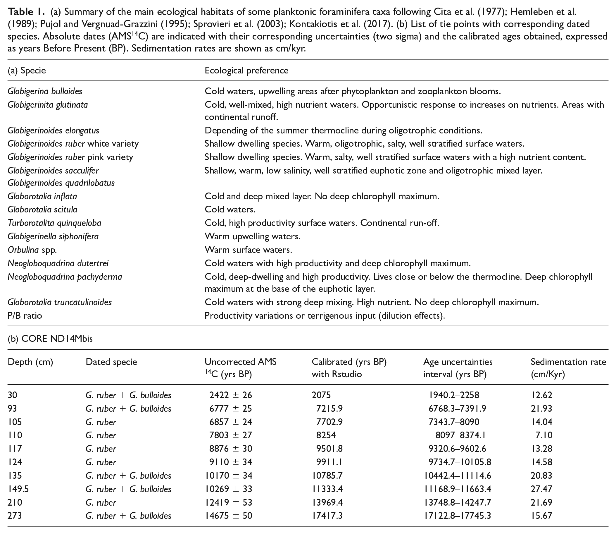
Some planktonic species have been grouped as follows: Globigerina bulloides, Globigerinita glutinata, Globigerinoides elongatus, Globigerinoides ruber divided in the white and the pink varieties, Globigerinoides quadrilobatus which includes Globigerinoides trilobus and Globigerinoides sacculifer, Globorotalia inflata, Globorotalia scitula distinguishing between left and right coiling, Turborotalita quinqueloba, Globigerinella siphonifera which includes Globigerinella calida, Orbulina spp. which includes Orbulina universa and O. suturalis, Neogloboquadrina dutertrei and, finally, Neogloboquadrina pachyderma and Globorotalia truncatulinoides distinguishing in both between left and right coiling. These species are represented in percentages of the total assemblage. In order to characterize environmental changes, the planktonic/benthic foraminifera ratio (P/B ratio) was also calculated and plotted.

Age model

The age model of core ND14Mbis is based on ten radiocarbon (¹⁴C) AMS measurements, seven of which were strategically selected along the S1 interval, including the pre- and post- intervals (Figure 2b). 3–6 mg per sample of monospecific G. ruber white variety (and G. bulloides in some cases) were handpicked from the >150 µm fraction (Table 1b). Samples were graphitized at the Godwin Laboratory for Palaeoclimate Research of the University of Cambridge (UK) following the protocol described on Freeman et al. (2016) and analysed at the ¹⁴CHRONO Centre of the Queen’s University of Belfast (UK). Radiocarbon ages were calibrated using MARINE13 calibration curves (Reimer et al., 2013) to account for global marine reservoir ages and to obtain calendar ages (cal yr BP), age correction for regional reservoir effects (ΔR) was not applied due to the lack of reliable estimates. The age model was constructed using the Bayesian statistics software Bacon with the statistical package R (Blaauw and Christien, 2011). Hereafter, the ND14Mbis calibrated ages are reported as kyrs.

Based on the constructed age model, the sedimentation rates were estimated to be ~26.3 cm/kyr for the pre-Sapropel period, ~15.9 cm/kyr for the S1a, ~5.4 cm/kyr for the S1i, ~8.3 cm/kyr for the S1b and ~25 cm/kyr for the post-Sapropel period (Table 1b). This is equivalent to a temporal sampling resolution of 38–185 year per sample, therefore allowing sub-millennial events in the sedimentary record to be inferred. In addition, focusing only on Sapropel S1 deposition, the mean sedimentation rate of the study core (~10 cm/kyr) is almost comparable with the sedimentation rate of other Sapropel S1 Mediterranean records, independently of the water depth, as follows: North Ionian Sea (~10 cm/kyr, Filippidi et al., 2016), North-east Ionian Sea (~5.5 cm/kyr, Geraga et al., 2008), Adriatic Sea (~20 cm/kyr, Mercone et al., 2000; Siani et al., 2010), South Aegean Sea (~10.3 cm/kyr, Casford et al., 2002), North Aegean Sea (~15.4 cm/kyr, Roussakis et al., 2004 and 17,3 cm/kyr Giamali et al., 2019) and Eastern Levantine basin (~20 cm/kyrs, Cornuault et al., 2018). On the other hand, our average sedimentation rates during the S1 are significantly different from other core sites with exceptionally high sedimentation rates in the North (67.6 cm/kyr, Kontakiotis, 2016) and South Aegean (~37.5 cm/kyr, Kontakiotis, 2016) Sea records. These differences in sedimentation rate from different sites of the Mediterranean could be related to several factors such as continental input, regional oceanography, water depth, deep currents lateral sediment transport, etc.

Results

Stable isotopes

The δ¹⁸O_G.ruber signal shows relatively heavy isotopic ratios (1.25–2.35‰) at the base of the studied interval (11.3–6 kyrs BP) followed by a trend towards lighter δ¹⁸O values that culminates at the onset of S1a (10 kyrs BP) with relatively light values (−0.22−0.95‰) (Figure 3a). This record has been compared with nearby deep-sea cores (Filippidi and De Lange, 2019; Geraga et al., 2008; Rohling et al., 2002 and Siani et al., 2010; Figure 3). To prevent age model discrepancies between core sites in the data comparison we have recalculated the radiocarbon age models for the published δ¹⁸O_G.ruber records following the same Bayesian age model approach adopted for the study core (cf. section 3.4). The comparison of the recalibrated stable isotope G. ruber records shows that in the study core (ND14Mbis) δ¹⁸O reaches the lighter interglacial values (–0.22–0.95‰) at 10 kyrs BP (Figure 3a), in Filippidi and De Lange (2019) at 10 kyrs BP (north Ionian Sea, Figure 3c), in Geraga et al. (2008) at 9.5 kyrs BP (north eastern Ionian Sea, Figure 3b), in Siani et al. (2010) at 9 kyrs BP (South Adriatic Sea, Figure 3d) and in Rohling et al. (2002) at 9.5 kyrs BP (South Aegean Sea, Figure 3e). All these records, show relatively constant δ¹⁸O values around −0.3–1.2‰ throughout the Early Holocene.

Figure 3.

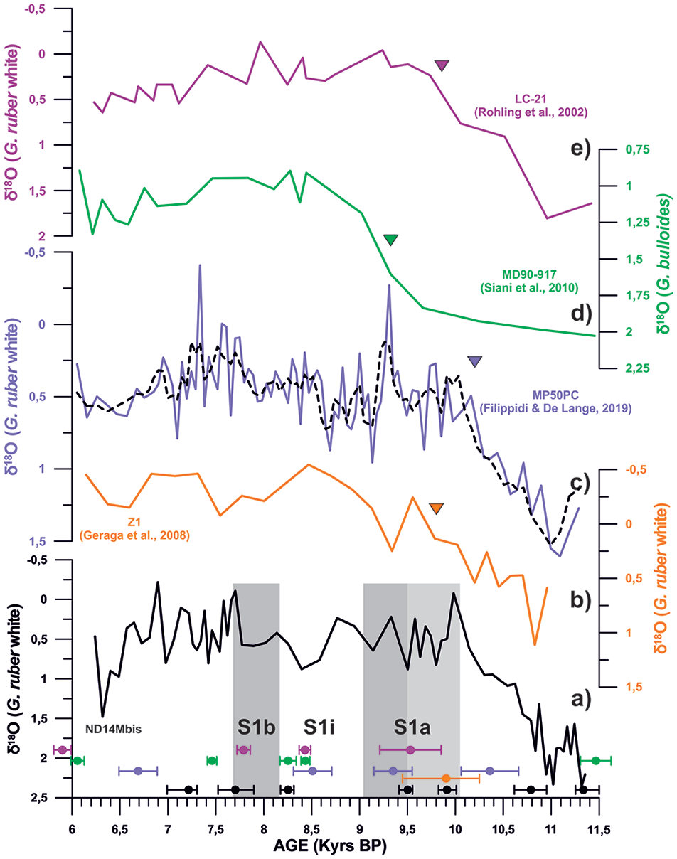
δ¹⁸O_G.ruber data of core ND14Mbis represented in black, compared to δ¹⁸O_G.ruber data from the north Ionian Sea of core Z1 (in orange, Geraga et al., 2008), core MP50PC (in purple and in black the mean values, Filippidi and De Lange, 2019) and the South Aegean Sea core LC-21 (in pink, Casford et al., 2002), andδ¹⁸O_G.bulloides data from core MD90-917 (in green, Siani et al., 2010), from the Adriatic Sea. Black, orange, purple, green and pink dots correspond to each tie point used in the age model of each core. The orange, purple, green and pink triangles correspond to the age of the beginning of the S1 deposition according to each author. The grey bars represent the S1a and S1b phase time intervals.

XRF analysis

Sapropel layers in sediments are typically expressed as distinct dark coloured layers, sometimes laminated and enriched in organic carbon. This feature makes for an easy recognizable trait of Sapropel layers. The 37 cm-length interval that was analysed at a higher resolution corresponds to these dark layers that can be seen at Figure 2a. We used the lightness values (L*) obtained from the high-resolution images of the sediments (taken with the Avaatech XRF core scanner) to identify the Sapropel unit and its interruption more precisely (Figure 2a). The marked decrease in the lightness values observed in this section marks the Sapropel layers on the core (Figures 4a and 5a). It has been shown at other Sapropel layers that dark colour bands are often slightly thicker than the interval defined by the organic carbon (De Lange et al., 1999). In our study core we clearly find a light dark coloured 2 cm thick layer (between 103 cm and105 cm) above the defined end of the sapropel unit based on our proxies, with a diffuse upper boundary and a relatively abrupt colour transition at its lower boundary (Figure 2a).

Figure 4.

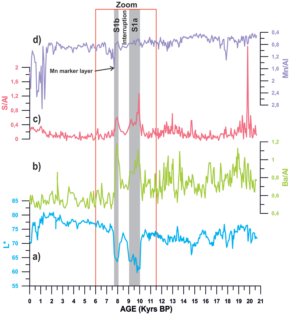
Records from core ND14Mbis of (a) lightness (1 cm resolution), (b) Barium/Aluminium ratio (Ba/Al), (c) Sulphur/Aluminium ratio (S/Al), and (d) Manganese/Aluminium ratio (Mn/Al). The red box represents the study period around sapropel 1, between 6 and 11.5 kyrs BP, and the grey bars mark S1a and S1b phases.

Figure 5.

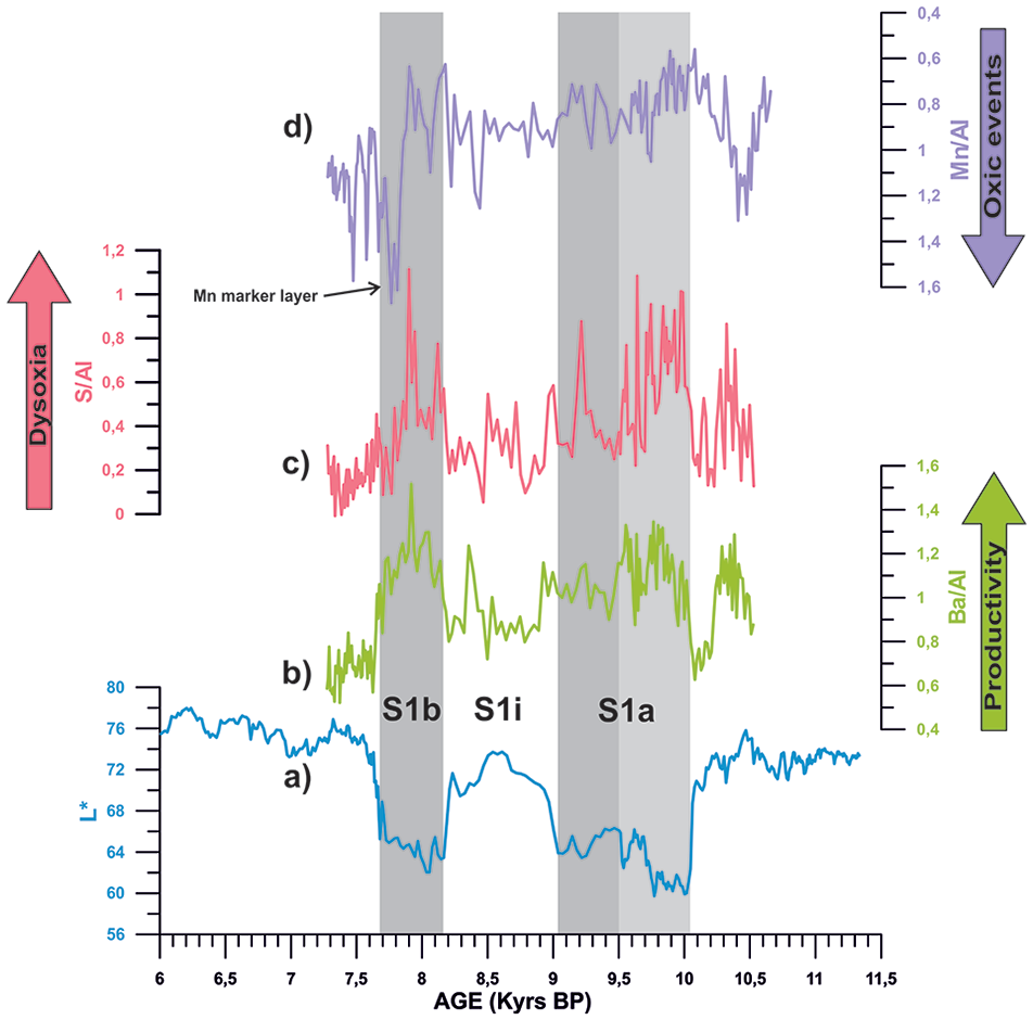
High-resolution (2 mm) XRF records from core ND14Mbis. (a) lightness, (b) Barium/Aluminium ratio (Ba/Al), (c) Sulphur/Aluminium ratios (S/Al), and (d) Manganese/Aluminium ratio (Mn/Al). This data corresponds to the studied period marked in red on Figure 5. Grey bars represent the S1a and S1b phase time intervals, while light grey bar shows the subdivision of S1a.

XRF elemental ratios such as Ba/Al and S/Al show particularly abrupt changes through S1a and S1b intervals, synchronous to lowest values of lightness record (Figures 4 and 5). During S1i, all these elemental ratios recover back to similar values than during pre-Sapropel times. After 7.7 kyrs BP (end of Sapropel deposition), all proxies recover their pre-Sapropel values again.

Planktonic foraminiferal assemblages

The relative percentage abundance of the most significant planktonic foraminiferal species recovered in core ND14Mbis between 11.5 and 6 kyrs BP is displayed in Figure 6. Over the studied time interval, the planktonic foraminifera were relatively abundant and well preserved. The planktonic foraminiferal assemblage was dominated by G. ruber white variety, G. inflata and N. pachyderma (right and left coiling), reaching abundances of 68.2, 42.3, and 30.6%, respectively.

Figure 6.

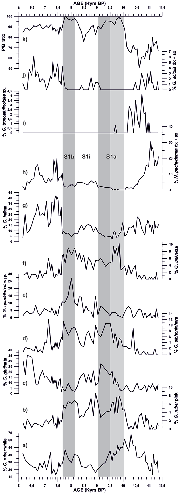
Records of planktonic foraminifera assemblages from core ND14Mbis for the 11.5–6 kyrs time interval. Grey bars represent the S1a and S1b phase time intervals, while light grey bar shows the subdivision of S1a.

The planktonic foraminifera G. ruber pink, G. siphonifera, G. quadrilobatus gr. and O. universa describe similar trends with high abundance values mainly during S1a and S1b (Figure 6). Conversely, they present lower values, before and after these two intervals, as well as during S1i (from 9 to 8.2 kyrs BP). G. ruber white has a distinctive behaviour with respect to the others, showing an earlier onset in the abundance increase at 11 kyrs BP and reaching its maximum peak at 10.3 kyrs BP (Figure 6a). At this point, G. ruber white abundance starts a decreasing trend until it reaches its lower values at 9 kyrs BP (end of S1a), while other warm water species (G. ruber pink, G. siphonifera and O. universa) present high abundance values. G. ruber white recovers high abundance values during S1b, presenting a similar trend to that of the rest of the warm water species, but with lower abundances than those recorded during S1a. Contrarily, G. ruber pink warm species resembles the same trend but presents a relative maximum peak at 8.9–8.8 kyrs BP (Figure 6b), when G. ruber white, G. siphonifera, G. quadrilobatus and O. universa were characterized by low relative abundances.

G. inflata presents a mean value of 7% in abundance during S1a and S1b phases, and increases in abundance to a mean value of 11.5% during S1i interval. With the ending of the Sapropel event (7.7 kyrs BP), G. inflata increases significantly reaching mean values of 25.8% (Figure 6g). N. pachyderma shows high relative abundances (15–31%) from 11.3 to 11 kyrs BP, then it starts a decreasing trend to 10.3 kyrs BP, in phase with G. ruber white increase (Figure 6a and 6h). From 10.3 kyrs BP and during S1a, N. pachyderma documents its lower values (0.3–1.4%), while during the S1i interval it documents a slightly increase in abundance to mean values of 3.5%. After the end of the Sapropel event, at 7.7 kyrs BP, the percentages of N. pachyderma show a marked increase in abundance to 22% (Figure 6h). G. scitula shows a peak of abundance ranging between 0 and 3.4% during the pre-Sapropel period, followed by its disappearance at the onset of S1a (10 kyrs BP) (Figure 6). Similar to N. pachyderma, G. scitula also presents a slight increase in abundance (0–2.2%) during S1i and during the post-Sapropel record (mean values of 2.2%). G. truncatulinoides shows peaks of abundance (mean values of 4.5%) during the pre-Sapropel period and then it abruptly disappears at 10.1 kyrs BP, at the onset of S1a (Figure 6i).

G. quadrilobatus gr. has a continuous distribution pattern with values ranging 0.5–8.5% with a prominent peak (27%) at 8 kyrs BP (Figure 6). G. glutinata shows very low abundances during S1a and S1b (2–10.3%) however, during S1i and between 9.5 and 8.2 kyrs (final part of S1a), this species has two increments in abundance of 10–20%. At 7.7 kyrs, with the end of the Sapropel period, G. glutinata shows a progressive increase in abundance reaching values of 35% (Figure 6c).

The P/B ratio shows an abrupt increase from values of 50–79%, during the pre-Sapropel phase, to 98.8% during S1a and 100% during S1b. It presents a slight reduction during S1i down to 75.8–91.2%. After 7.7 kyrs BP (at the end of the Sapropel interval deposition), the P/B ratio values decrease to 85.5–92%. When comparing the P/B ratio values during the pre-Sapropel period (before 10 kyrs BP) with the post-Sapropel period (after 7.7 kyrs BP), it can be determined that the P/B ratio after the Sapropel resulted higher than the pre-Sapropel one (Figure 6k).

Discussion

A combined approach based on the integration of different paleoclimatic proxy signals (L*, planktonic foraminiferal assemblages, δ¹⁸O records and XRF data) was used to identify and characterize S1 within a robust chronological constrain (Figure 7). In particular, we identified the following phases: S1a (10–9 kyrs BP), an interruption phase or S1i (9–8.2 kyrs BP), and S1b (8.2–7.7 kyrs BP). We defined the onset of the Sapropel taking as reference the first abrupt decrease of the L* signal (Figures 4a and 5a), associated with the disappearance of the planktonic foraminifera G. truncatulinoides (Figure 7d), at 10 kyrs BP. The end of S1 interval occurs at 7.7 kyrs BP, when L* values increase again.

Figure 7.

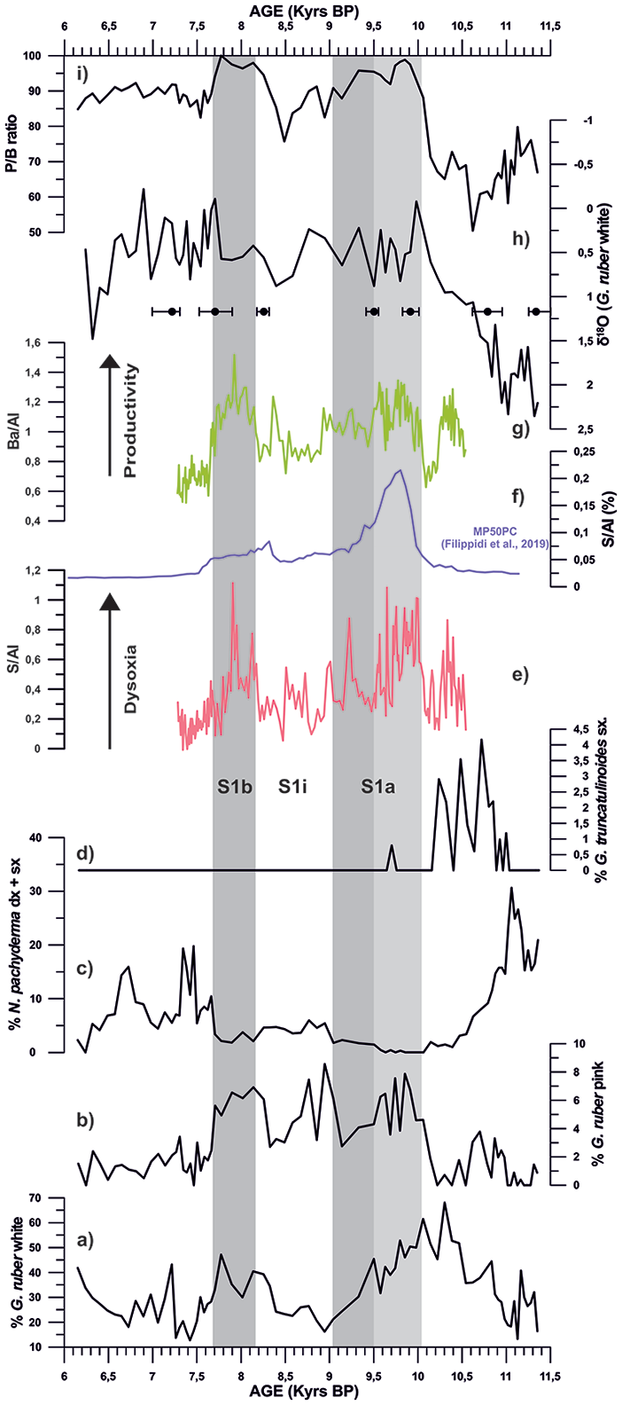
Records from core ND14Mbis of (a) Globigerinoides ruber white, (b) Globigerinoides ruber pink, (c) Neogloboquadrina pachyderma, (d) Globorotalia truncatulinoides, (e) Sulphur/Aluminium ratio (S/Al), (f) Sulphur/Aluminium ratio (S/Al) from core MP50PC (in purple, Filippidi et al., 2019), (g) Barium/Aluminium ratio (Ba/Al), (h) δ¹⁸O_G.ruber data of core ND14Mbis (i) Planktonic/Benthic foraminifera ratio (P/B ratio). Grey bars represent the S1a and S1b phase time intervals, while light grey bar shows the subdivision of S1a.

Pre-Sapropel interval: pre-S1 (11.3–10 kyrs BP)

The time interval before S1 deposition (pre-S1) was a period characterized by a series of hydrographic changes in surface water conditions that acted as pre-conditioning factors for the S1 deposition in the Ionian Sea. This period corresponds to the onset of the Holocene after the deglaciation period (dated at 11.7 kyrs BP, Walker et al., 2018). This suggested paleoceanographic framework can be confirmed by the δ¹⁸O data shown in Figure 7h.

δ¹⁸O_G.ruber data of our study core shows a 2.2‰ transition interval from heavy to light values during the pre-Sapropel interval (11.3–10 kyrs BP), corresponding to the global sea level rise after the YD event (Grant et al., 2016) followed by relatively stable and light δ¹⁸O_G.ruber values during the Holocene (Figure 7h). The pattern of our study record is comparable to other δ¹⁸O records in the Eastern Mediterranean basin (Figure 3). However, we find that our light δ¹⁸O values are achieved during the pre-S1, at 10 kyrs BP, while on the other sites light isotopic values happened at the beginning of S1 deposition; on the North Ionian record (Filippidi and De Lange, 2019) at 10 kyrs BP, on the North-eastern Ionian record (Geraga et al., 2008) at 9.5 kyrs BP, on the Southern Aegean Sea record (Rohling et al., 2002) at 9.5 kyrs BP and on the South Adriatic record (Siani et al., 2010) at 9 kyrs BP (Figure 3). However, for Geraga et al. (2008) this 500 yr discrepancy could be attributed to weak chronological constraints since the age model for this record has only one sample dated by radiocarbon during the sapropel event (Figure 3). These differences on the δ¹⁸O_G.ruber depletion age, between different cores (Ionian, Adriatic, and Aegean Sea), have already been described by other authors, who determined that the onset of the Sapropel layer deposition throughout the eastern Mediterranean Sea was not synchronous, irrespectively of the water depth deposition (10.8 ±0.4–6.1 ±0.5 Kyrs BP; De Lange et al., 2008; Incarbona et al., 2019). In spite of this asynchronicity, the similarities between the δ¹⁸O data of the four cores confirm the consistency of the age model for our study core within the ¹⁴C age uncertainty (Figure 3).

In the study core, the main planktonic foraminiferal change during this interval is the antithetic distribution patterns between G. ruber white and N. pachyderma (Figures 7a and c). In particular, G. ruber white, indicator of stratified (Principato et al., 2003), warm and oligotrophic surface waters (Hemleben et al., 1989; Zaric et al., 2005), shows a progressive abundance increase during the pre-S1, reaching maximum values at 10.3 kyrs BP. This species is associated with the presence of G. ruber pink, strongly suggesting stratified surface water conditions. Conversely, N. pachyderma, a deep dweller cold-water species linked to winter/spring high productivity and to a distinct deep chlorophyll maximum layer (Rohling and Gieskes, 1989), shows a decreasing abundance trend over the pre-S1 interval. This antithetic planktonic foraminiferal signature, previously documented in the Sicily Channel (Sprovieri et al., 2003), in the Gulf of Taranto (Di Donato et al., 2019), in the North eastern Ionian Sea (Geraga et al., 2008) and the Aegean Sea (Kontakiotis et al., 2009, 2013; Kontakiotis, 2016), suggests the gradual development of stratiﬁed and oligotrophic surface waters. In particular, high abundance of N. pachyderma, between 11.3 and 10.9 kyrs BP, suggests a well-developed deep Chlorophyll maximum and probably represents the end of the cooling related to the Younger Dryas event (i.e. Sprovieri et al., 2003; Di Donato et al., 2019). Upwards, peaks in abundance of G. inflata and G. truncatulinoides associated with G. scitula (Figures 6g, I, and j) suggest prevailing cool and deep vertical mixing conditions during winter (Hemleben et al., 1989; Pujol and Vergnaud-Grazzini, 1995). From 10.3 kyr BP, a sharp increase in the abundance of G. ruber white, associated with a sharp decrease of G. inﬂata and G. truncatulinoides, suggest the beginning of enhanced stratification of the water column. This micropaleontological signature is also associated with a gradual decrease in P/B ratio present both on our study core and on core MP50PC (Filippidi et al., 2016), located very close to our study area (North Ionian Sea), implying a progressive decrease in bottom waters oxygen concentration. According to these planktonic foraminiferal assemblages, we interpret the pre-Sapropel interval as a period with strong seasonality, having warm stratified surface water conditions but with winters characterized by colder waters and enhanced vertical mixing in the water column. The increased stratification could be the result of the entrance of freshwater and decreased surface water density. Plausible scenarios for the increased freshwater input suggest a combination of both post-glacial freshening, with the entrance of a less salty inflow from the Atlantic waters, and the African monsoon, with the increase of the rivers inflow and precipitations (Casford et al., 2002; Cita et al., 1977; De Lange et al., 1999, 2008; Di Donato et al., 2019; Rohling 1994; Rohling et al., 1997, 2015).

Sapropel interval: S1a (10–9 kyrs BP)

The onset of S1a interval occurs at 10 kyrs BP and is marked by the disappearance of G. truncatulinoides (Geraga et al., 2008; Sprovieri et al., 2003). This S1a interval is also characterised by the increase in abundance of warm planktonic foraminiferal species (G. ruber pink, G. quadrilobatus gr. and O. universa) and the low abundance (or absence) of cold planktonic foraminiferal ones (N. pachyderma, G. truncatulinoides, G. inflata and G. scitula), suggesting a progressive stratification of the water column (Figure 6). One of the main planktonic foraminiferal features over the S1 deposition is the strong increase in abundance of G. ruber pink (Figure 7b). This feature has been previously documented by several authors (Casford et al., 2007; Geraga et al., 2008; Siani et al., 2010) in different areas of the eastern Mediterranean (south and north-east Ionian Sea, east of Crete Island, south Aegean Sea). In particular, our records show an evident replacement of G. ruber white distribution pattern by G. ruber pink from 10 to 9.5 kyrs BP (Figure 7a and b) indicating a possible sub-phase inside S1a. This ecological feature could suggest a shift from an oligotrophic environment to eutrophic conditions, related to the ecological preferences of these species to warm, stratified surface waters (Hemleben et al., 1989; Pujol and Vergnaud-Grazzini, 1995). High abundance values of G. ruber pink result in phase with maximum Ba/Al values (Figures 7b and g). The Ba enrichment in sediments is also interpreted an increased productivity. In fact, Ba/Al ratio (Figure 7g), measured both in foraminiferal tests and bulk sediments (Antonarakou et al., 2015; Hönisch et al., 2011), is considered as paleo-productivity proxy (i.e. Gallego-Torres et al., 2007; Martínez-Ruiz et al., 2000). According to this latter Ba/Al interpretation and its agreement with the G. ruber pink record, we could confirm a high productivity interval between 10 and 9.5 kyr BP that we defined as the first sub-phase of S1a. The parallelism between G. ruber pink and Ba/Al record states a progressive decrease in productivity versus the end of S1a interval (9.5–9 kyr BP; second sub-phase of S1a). In this study, Ba/Al record is very similar to the ones on core MP50PC (north Ionian Sea) of Filippidi et al. (2016).

The opportunistic planktonic foraminiferal species G. glutinata shows low values during the beginning of S1a interval (average of 5%), however, from 9.5 to 9 kyrs BP (during the second sub-phase of S1a) presents an abrupt increase in abundance up to 27.5% (Figure 6c). This species is linked to a local rapid nutrient increase and is a specialist diatom feeder, thus being particularly abundant in areas with high continental runoff and high river input; this species can survive on a wide thermal range and within the deep surface mixed layer (Hemleben et al., 1989). The concomitant increase in abundance of G. glutinata and G. siphonifera seems to suggest the shift at the end of S1a interval to relatively well-mixed water masses during the winter season (Rohling et al., 2004). We argue that during the second S1a sub-phase, the stratification of the water column might have decreased slightly, resulting in a replacement of G. ruber pink by G. glutinata, since this species has a wider range of adaptability.

The increase of P/B ratio during S1a (Figure 7i) suggests dysoxic conditions on the bottom waters, since these are not suitable conditions for the proliferation of benthic foraminiferal species. The low oxygen concentration in deep waters could be the result of high nutrient content during a time of surface water stratification. These conditions allowed to the organic matter to be transported downward in the water column and deposited. The respiration of this organic matter by bacteria together with reduced deep water ventilation as a result of the stratified surface waters eventually established the dysoxic conditions necessary to preserve the organic matter and therefore the formation of the Sapropel layer. We interpret the waters as being dysoxic and not anoxic because the benthic foraminiferal fauna (Cassidulinoides brady, Gyroidina spp., Miliolids, Planulina ariminensis, Cibicides spp., Cibicidoides spp. and Planulina spp.) does not completely disappear, being present in almost all the samples even if it is in low proportions (Figure 7i). This hypothesis is also supported by the similar P/B ratio in core MP50PC (Filippidi et al., 2016) and by the higher values shown by our S/Al record and in core MP50PC (Filippidi et al., 2016) during S1a (Figure 7e and f). Sulphur is attributed to pyrite formation that precipitates during reducing conditions (low oxygen) in the bottom waters (Filippidi et al., 2016). According to the P/B and S/Al ratios on both our core and on Filippidi et al. (2016), the second sub-phase of S1a (9.5–9 kyrs BP) was less dysoxic than the first one (10–9.5 kyrs BP), likely due to relatively less productivity than the first sub-phase (as described by G. ruber pink and Ba/Al) and less stratification (as described by G. glutinata).

Sapropel interruption: S1i (9–8.2 kyrs BP)

The main planktonic foraminiferal signature during the Sapropel interruption (S1i; 9–8.2 kyrs BP) is a general increase in abundance of the cold-water species G. inflata and N. pachyderma. The increase of these two species, indicative of a well-developed thick and cold mixed layers and formation of a deep chlorophyll maximum layer (Pujol and Vergnaud Grazzini, 1995) has been previously documented by several authors in the Eastern Mediterranean Basin (Casford et al., 2001; Geraga et al., 2008, 2010; Giamali et al., 2019; Kontakiotis et al., 2013; Kontakiotis, 2016; Lirer et al., 2013; Principato et al., 2003; Siani et al., 2010; Sprovieri et al., 2003; Triantaphyllou et al., 2009). The concomitant decrease in abundance of warm water planktonic foraminifera G. ruber white and O. universa with the slightly heavier values in δ¹⁸O G. ruber signal, describe the S1i as a relatively colder period. In addition, during this sapropel interruption (S1i) phase, the increase in benthic foraminiferal species, documented by a shift in P/B ratio, as also reported in Filippidi et al. (2016) in the Ionian Sea record, suggests an improvement of the bottom water conditions for the proliferation of those benthic species (Figure 7i). These planktonic and benthic foraminiferal signals document a re-ventilation of the deep waters linked to mixing processes, thus giving further arguments in favour of the possible entry of colder waters. These new paleoceanographic conditions are in agreement with the decrease in sulphur (S/Al, Figure 7e and f) signature during S1i, suggesting less pyrite formation, hence more oxygen content in the bottom waters, defining a partial re-oxygenation. The entry of these colder waters could have been at an intermediate depth, since the mixing had effects on both the surface and the deep waters. In addition, the Ba/Al record show lower values suggesting a decreasing input of productivity (Figure 7g).

A peculiar planktonic foraminiferal feature, occurring during S1i interval, is the presence of G. ruber pink with a relative maximum peak at 8.9–8.7 kyrs BP. This signature has not been documented in any other Mediterranean cores and due to a lack of additional data, we have no further insight on why this feature appears on our core. Despite the cause being unknown and the lack of data to support our hypothesis, we can suggest a possible scenario for the appearance of this species during S1i. G. ruber pink variety occurs preferentially at the end of summer (Pujol and Vergnaud-Grazzini, 1995), thus the peak on our data could be interpreted as the result of seasonal resilient stratification that helped preserve warmer waters at a surface level. Core Z1 (Geraga et al., 2008) is located near our core but it does not present this feature, thus we interpret that this phenomenon must have been occurring very locally, and is not particular of whole Ionian Sea.

Sapropel interval: S1b (8.2–7.7 kyrs BP)

S1b interval (8.2–7.7 kyrs BP) is defined by an increase of warm planktonic foraminiferal species (i.e. G. ruber white, G. ruber pink, G. quadrilobatus gr. and O. universa) and a decrease of cold ones (i.e. G. inflata and N. pachyderma) (Figure 6). According to the increase in abundance of G. ruber pink (Figure 7b) and the increase in Ba/Al ratio (Figure 7g), S1b interval can be characterized by high nutrient content, also visible with the darker colour of the sapropel layer described by the lightness values (Figures 4a and 5a). The strong increase in abundance of G. quadrilobatus gr. and O. universa, over the S1b phase, as previously documented in the eastern Ionian Sea (Geraga et al., 2008), and the Aegean Sea (Giamali et al., 2019; Kontakiotis, 2016; Kontakiotis et al., 2013; Triantaphyllou et al., 2009), suggests the presence of an extended warm climate conditions and mixed layer during summer season (i.e. Pujol and Vergnaud Grazzini, 1995). In addition, the occurrence of G. siphonifera, might state well-mixed water masses during winter season (Rohling et al., 2004).

High values of the P/B ratio during S1b interval (comparable to Those of Filippidi et al., 2016), together with an increase of the S/Al record (Figures 7e, f, and i), suggest dysoxic bottom waters conditions, similar to that documented in the first sub-phase of S1a interval. In addition, we suggest that the main source area of nutrients over S1b interval was the increased river runoff, as stated during S1a, even if G. glutinata has very low abundance values. The high stratification of the water column during S1b, similar to that of the first sub-phase of S1a (as described by the P/B ratio and S/Al), could have allowed the proliferation of G. ruber pink not giving space to G. glutinata opportunistic species to occupy its biological niche. In fact, this antagonistic distribution pattern between G. ruber pink and G. glutinata characterize the entire sapropel event.

Post-Sapropel interval: post-S1 (post 7.7 kyrs BP)

From 7.7 kyr BP upwards (post-sapropel period), there is a strong and sudden recovery in the abundance of cold-water species (G. inflata, N. pachyderma and G. scitula) whereas the warm water ones (G. ruber white, G. ruber pink, G. quadrilobatus gr. and O. universa) describe an opposite trend (Figure 6). This abrupt change in the planktonic foraminiferal assemblage and the strong decrease in the Ba/Al records (similar to Filippidi et al., 2016) mark the end of the stagnation and high productivity period, therefore ending S1 (Figure 7g), marking the onset of the re-establishment of cool water conditions and vertical mixing during the winter. The P/B ratio (Figure 7i) associated with the depletion in S/Al signal (Figures 7e and f) shows values similar to that documented during the Sapropel S1i and it never recovers the well-oxygenated deep water conditions as during the pre-Sapropel deposition. In addition, a strong increase in Mn/Al ratio at 7.8 kyrs BP (Figure 5d), marks the occurrence of the manganese marker layer, a well-documented layer of variable thickness (between 2–3 cm) that overlies most sapropel layers in the eastern Mediterranean Sea (De Lange et al., 1999; Filippidi and De Lange, 2019; Martinez-Ruiz et al., 2000; Mercone et al., 2000; Meier et al., 2004; Thomson et al., 1999). This Mn-rich layer has a light dark colour characteristic from sediments enriched with Mn and a 2 cm thickness, a diffuse upper boundary and a relatively abrupt colour transition at its lower boundary (Figure 2a). It was formed when, after the sapropel event, the dysoxic deep waters were re-ventilated, since Mn is present in the soluble form under dysoxic conditions but it precipitates when oxygen is added (Martinez-Ruiz et al., 2000; Meier et al., 2004; Thomson et al., 1995, 1999), thus additional Mn peaks can be found.

Conclusion

We present a high-resolution paleoceanographic reconstruction based on a multi-proxy approach of the most recent sapropel event (S1) (10–7.7 kyrs BP) in a 655 m water depth record from the North Ionian Sea (eastern Mediterranean Sea). The ecological interpretation of planktonic foraminiferal assemblages, integrated with the XRF elemental data and oxygen isotope G. ruber record have provided an accurate interpretation of the changes in surface water properties. The results allowed us to divide S1 into different phases, starting with a preconditioning period (pre-S1) from 11.3 to 10 kyrs BP. We define the pre-S1 as a period with strong seasonality, having warm stratified surface water conditions but with colder winters characterized by an intensification of vertical mixing in the water column. A progressive increase of P/B ratio also suggests a depletion of oxygen concentration of the bottom water. Later, S1 interval has been divided into two warm phases, S1a (10–9 kyrs BP) and S1b (8.2–7.7 kyrs BP), separated by a cold interruption event, S1i (9–8.2 kyrs BP). Proxies of paleo-productivity (G. ruber pink and Ba/Al) and proxies linked to mixing of the water column (G. ruber white and N. pachyderma) indicate that S1a and S1b were characterized by stratified surface waters rich in nutrient content. The deposition of S1a started at 10 kyrs BP with an increase in nutrients related to the river runoff. P/B ratio and S/Al records allowed to define S1a and S1b as dysoxic events. The interruption of S1 (S1i) is characterized by the entrance of colder waters that caused mixing of the stratified water column and re-ventilated of the deep dysoxic waters. The high resolution of our record allowed the identification of a two sub-phases into the S1a interval, being the first sub-phase (10–9.5 kyrs BP) characterized by high productivity, strong stratification and dysoxic deep waters, while the second sub-phase (9.5–9 kyrs BP) by less productivity and a slightly decreased level of stratification that caused less dysoxic deep waters. We conclude that S1 was the result of a complex interaction of different oceanographic processes triggered by the arrival of fresh nutrient-rich waters that caused dysoxia on the deep ocean waters.

Footnotes

Acknowledgements

We thank Maria de la Fuente (University of Barcelona, Spain), Luke Skinner (Godwin Laboratory for Palaeoclimate Research, University of Cambridge, UK) and Ron Reimer (¹⁴Chrono Centre, Queen’s University of Belfast, UK) for providing the ¹⁴C AMS data for the age model. We thank José Noel Pérez-Asensio for providing the data of the benthic foraminifera assemblages present on the study core. L.D. Pena acknowledges support from the CTM2016-75411 project and from the Ramón y Cajal program (MINECO, Spain). We also thank Amalia Filippidi, Maria Geraga and Giuseppe Siani for sharing their δ¹⁸O data from each of their articles. The Generalitat de Catalunya is grateful for its support through its program on Grups de Recerca Consolidats (grant 2017 SGR 315 to GRC Geociències Marines) its program on Serra Húnter Tenure-eligible Lecturer contract (J. Frigola) and its ICREA-Academia program (I. Cacho). Finally, we want to thank Dr. George Kontakiotis and anonymous reviewer for reviewing this paper and for their helpful suggestions that helped improve the manuscript.

Funding

The author(s) disclosed receipt of the following financial support for the research, authorship, and/or publication of this article: The core ND14Mbis has been collected by ISMAR-CNR (Napoli) aboard of the CNR-Urania vessel during the oceanographic cruise NEXTDATA-2014, therefore we want to thank them for collecting the study core. This research has been financially supported by the TIMED Project funded by the European Commission (ERC Consolidator Grant; ID: 683237) and the Project of Strategic Interest NextData PNR 2011–2013 ().

ORCID iD

Helena Checa

References

Abu-Zied

Rohling

Jorissen

, et al. (2008) Benthic foraminiferal response to changes in bottom-water oxygenation and organic carbon flux in the eastern Mediterranean during LGM to Recent times. Marine Micropaleontology 67(1): 46–68.

Antonarakou

Kontakiotis

Mortyn

, et al. (2015) Biotic and geochemical (δ18O, δ13C, Mg/Ca, Ba/Ca) responses of Globigerinoides ruber morphotypes to upper water column variations during the last deglaciation, Gulf of Mexico. Geochimica et Cosmochimica Acta 170: 69–93.

Antonarakou

Kontakiotis

Karageorgis

, et al. (2019) Eco-biostratigraphic advances on late Quaternary geochronology and paleoclimate: The marginal Gulf of Mexico analogue. Geological Quarterly 63(1): 178–191.

Antonarakou

Kontakiotis

Zarkogiannis

, et al. (2018) Planktonic foraminiferal abnormalities in coastal and open marine eastern Mediterranean environments: A natural stress monitoring approach in recent and early Holocene marine systems. Journal of Marine Systems 181: 63–78.

Bazzicalupo

Maiorano

Girone

, et al. (2020) Holocene climate variability of the Western Mediterranean: Surface water dynamics inferred from calcareous plankton assemblages. The Holocene 30(5): 691–708.

Blaauw

Christen

(2011) Flexible paleoclimate age-depth models using an autoregressive gamma process. Bayesian Analysis 6(3): 457–474.

Cacho

Grimalt

Canals

, et al. (2001) Variability of the western Mediterranean Sea surface temperature during the last 25,000 years and its connection with the Northern Hemisphere climatic changes. Paleoceanography 16(1): 40–52.

Calvert

Fontugne

(2001) On the late Pleistocene-Holocene Sapropel record of climatic and oceanographic variability in the eastern Mediterranean. Paleoceanography 16(1): 78–94.

Calvert

Pedersen

(2007) Chapter fourteen elemental proxies for palaeoclimatic and palaeoceanographic variability in marine sediments: Interpretation and application. Developments in Marine Geology 1: 567–644.

10.

Casford

JSL

Abu-Zied

Rohling

, et al. (2007) A stratigraphically controlled multiproxy chronostratigraphy for the eastern Mediterranean. Paleoceanography 22(4): 4215.

11.

Casford

JSL

Rohling

Abu-Zied

, et al. (2002) Circulation changes and nutrient concentrations in the Late Quaternary Aegean Sea: A non-steady state concept for Sapropel formation. Paleoceanography 17(2): 14–1.

12.

Casford

JSL

Rohling

Abu-Zied

, et al. (2003) A dynamic concept for eastern Mediterranean circulation and oxygenation during sapropel formation. Palaeogeography, Palaeoclimatology, Palaeoecology 190: 103–119.

13.

Cita

Vergnaud-Grazzini

Robert

, et al. (1977) Paleoclimatic record of a long deep sea core from the Eastern Mediterranean. Quaternary Research 8(2): 205–235.

14.

Coplen

(1996) New guidelines for the reporting of stable hydrogen, carbon, and oxygen isotope ratio data. Geochimica et Cosmochimica Acta 60(17): 3359–3360.

15.

Cornuault

Tachikawa

Vidal

, et al. (2018) Circulation changes in the Eastern Mediterranean Sea over the past 23,000 years inferred from authigenic Nd isotopic ratios. Paleoceanography and Paleoclimatology 33(3): 264–280.

16.

Cushman-Roisin

Gacic

Poulain

, et al. (2001) Physical Oceanography of the Adriatic Sea: Past, Present and Future. Leeds: Springer-Science + Business Media, BV.

17.

Di Donato

Insinga

Iorio

, et al. (2019) The palaeoclimatic and palaeoceanographic history of the Gulf of Taranto (Mediterranean Sea) in the last 15 ky. Global and Planetary Change 172: 278–297.

18.

De Lange

Thomson

Reitz

, et al. (2008) Synchronous basin-wide formation and redox-controlled preservation of a Mediterranean Sapropel. Nature Geoscience 1(9): 606–610.

19.

De Lange

Van Santvoort

PJM

Langereis

, et al. (1999) Paleo-environmental variations in eastern Mediterranean sediments: A multidisciplinary approach in a prehistoric setting. Progress in Oceanography 44(1–3): 369–386.

20.

De Rijk

Hayes

Rohling

(1999) Eastern Mediterranean sapropel S1 interruption: An expression of the onset of climatic deterioration around 7 ka BP. Marine Geology 153(1–4): 337–343.

21.

Drinia

Antonarakou

Tsourou

, et al. (2016) Foraminifera eco-biostratigraphy of the southern Evoikos outer shelf, central Aegean Sea, during MIS 5 to present. Continental Shelf Research 126: 36–49.

22.

Filippidi

De Lange

(2019) Eastern Mediterranean deep water formation during sapropel S1: A reconstruction using geochemical records along a bathymetric transect in the Adriatic outflow region. Paleoceanography and Paleoclimatology 34(3): 409–429.

23.

Filippidi

Triantaphyllou

De Lange

(2016) Eastern-Mediterranean ventilation variability during Sapropel S1 formation, evaluated at two sites influenced by deep-water formation from Adriatic and Aegean Seas. Quaternary Science Reviews 144: 95–106.

24.

Freeman

Skinner

Reimer

, et al. (2016) Graphitization of small carbonate samples for paleoceanographic research at the godwin radiocarbon laboratory, University of Cambridge. Radiocarbon 58(1): 89–97.

25.

Gallego-Torres

Martínez-Ruiz

Paytan

, et al. (2007) Pliocene–Holocene evolution of depositional conditions in the eastern Mediterranean: Role of anoxia vs productivity at time of Sapropel deposition. Paleogeography, Paleoclimatology, Paleoecology 246(2–4): 424–439.

26.

Garcia-Solsona

Pena

Paredes

, et al. (2020) Rare Earth Elements and Nd isotopes as tracers of modern ocean circulation in the central Mediterranean Sea. Progress in oceanography 185: 102340.

27.

Geraga

Ioakim

Lykousis

, et al. (2010) The high-resolution palaeoclimatic and palaeoceanographic history of the last 24,000 years in the central Aegean Sea, Greece. Palaeogeography Palaeoclimatology Palaeoecology 287(1–4): 101–115.

28.

Geraga

Mylona

Tsaila-Monopoli

, et al. (2008) Northeastern Ionian Sea: Paleoceanographic variability over the last 22 ka. Journal of Marine Systems 74(1–2): 623–638.

29.

Giamali

Koskeridou

Antonarakou

, et al. (2019) Multiproxy ecosystem response of abrupt Holocene climatic changes in the north-eastern Mediterranean sedimentary archive and hydrologic regime. Quaternary Research 92(3): 665–685.

30.

Grant

Grimm

Mikolajewicz

, et al. (2016) The timing of Mediterranean sapropel deposition relative to insolation, sea-level and African monsoon changes. Quaternary Science Reviews 140: 125–141.

31.

Grimm

Maier-Reimer

Mikolajewicz

, et al. (2015) Late glacial initiation of Holocene eastern Mediterranean Sapropel formation. Nature Communications 6(1): 1–12.

32.

Hemleben

Spindler

Anderson

(1989) Modern Planktonic Foraminifera. Leeds: Springer- Verlag.

33.

Hennekam

Jilbert

Schnetger

, et al. (2014) Solar forcing of Nile discharge and sapropel S1 formation in the early to middle Holocene eastern Mediterranean. Paleoceanography 29(5): 343–356.

34.

Hönisch

Allen

Russell

, et al. (2011) Planktic foraminifers as recorders of seawater Ba/Ca. Marine Micropaleontology 79(1–2): 52–57.

35.

Incarbona

Abu-Zied

Rohling

, et al. (2019) Reventilation episodes during the sapropel S1 deposition in the Eastern Mediterranean based on holococcolith preservation. Paleoceanography and Paleoclimatology 34(10): 1597–1609.

36.

Kallel

Duplessy

Labeyrie

, et al. (2000) Mediterranean pluvial periods and Sapropel formation over the last 200.000 years. Palaeogeography, Palaeoclimatology, Palaeoecology 157(1–2): 45–58.

37.

Klein

Wolfgang

Civitarese

, et al. (2000) Is the Adriatic returning to dominate the production of Eastern Mediterranean Deep Water? Geophysical Research letters 27(20): 3377–3380.

38.

Kontakiotis

(2016) Late Quaternary paleoenvironmental reconstruction and paleoclimatic implications of the Aegean Sea (eastern Mediterranean) based on paleoceanographic indexes and stable isotopes. Quaternary International 401: 28–42.

39.

Kontakiotis

Antonarakou

Zachariasse

(2013) Late Quaternary palaeoenvironmental changes in the Aegean Sea: Interrelations and interactions between North and South Aegean Sea. Bulletin of the Geological Society of Greece 47(1): 167–177.

40.

Kontakiotis

Antonarakou

Mortyn

, et al. (2017) Morphological recognition of Globigerinoides ruber morphotypes and their susceptibility to diagenetic alteration in the eastern Mediterranean Sea. Journal of Marine Systems 174: 12–24.

41.

Kontakiotis

Antonarakou

Triantaphyllou

, et al. (2009) Planktonic foraminiferal Mg/Ca as a proxy for paleoceanographic reconstruction during deposition of Holocene S1 sapropel in Aegean Sea. Proceedings of 9th Symposium on Oceanography and Fishery 1: 73–78.

42.

Kotthoff

Pross

Müller

, et al. (2008) Climate dynamics in the borderlands of the Aegean Sea during formation of sapropel S1 deduced from a marine pollen record. Quaternary Science Reviews 27(7–8): 832–845.

43.

Koutrouli

Anastasakis

Kontakiotis

, et al. (2018) The early to mid-Holocene marine tephrostratigraphic record in the Nisyros-Yali-Kos volcanic center, SE Aegean Sea. Journal of Volcanology and Geothermal Research 366: 96–111.

44.

Le Houedec

Mojtahid

Bicchi

, et al. (2020) Suborbital hydrological variability inferred from coupled benthic and planktic foraminiferal-based proxies in the south-eastern Mediterranean during the last 19 ka. Paleoceanography and Paleoclimatology 35(2): e2019PA003827.

45.

Lirer

Sprovieri

Ferraro

, et al. (2013) Integrated stratigraphy for the Late Quaternary in the eastern Tyrrhenian Sea. Quaternary International 292: 71–85.

46.

Louvari

Drinia

Kontakiotis

, et al. (2019) Impact of latest-glacial to Holocene sea-level oscillations on central Aegean shelf ecosystems: A benthic foraminiferal palaeoenvironmental assessment of South Evoikos Gulf, Greece. Journal of Marine System 199: 103181.

47.

Manca

Budillon

Scarazzato

, et al. (2003) Evolution of dynamics in the eastern Mediterranean affecting water mass structures and properties in the Ionian and Adriatic Seas. Journal of Geophysical Research 108(C9): 8102.

48.

Margaritelli

Cisneros

Cacho

et al. (2018) Climatic variability over the last 3000 years in the central – western Mediterranean Sea (Menorca basin) detected by planktonic foraminifera and stable isotope records. Global and Planetary Change 169: 179–187.

49.

Marino

Rohling

Sangiorgi

, et al. (2009) Early and middle Holocene in the Aegean Sea: Interplay between high and low latitude climate variability. Quaternary Science Reviews 28(27): 3246–3262.

50.

Martinez-Ruiz

Kastner

Paytan

, et al. (2000) Geochemical evidence for enhanced productivity during S1 Sapropel deposition in the eastern Mediterranean. Paleoceanography 15(2): 200–209.

51.

Mélières

Rossignol-Strick

Malaizé

(1997) Relation between low latitude insolation and δ18O change of atmospheric oxygen for the last 200 kyrs, as revealed by Mediterranean Sapropels. Geophysical Research Letters 24(10): 1235–1238.

52.

Meier

KJS

Zonneveld

KAF

Kasten

, et al. (2004) Different nutrient sources forcing increased productivity during eastern Mediterranean S1 Sapropel formation as reflected by calcareous dinoflagellate cysts. Paleoceanography 19(1): PA1012.

53.

Mercone

Thomson

Abu-Zied

, et al. (2001) High resolution geochemical and micro-palaeontological profiling of the most recent eastern Mediterranean Sapropel. Marine Geology 177(1–2): 25–44.

54.

Mercone

Thomson

Croudace

, et al. (2000) Duration of S1, the most recent sapropel in the eastern Mediterranean Sea, as indicated by accelerator mass spectrometry radiocarbon and geochemical evidence. Paleoceanography 15(3): 336–347.

55.

Mojtahid

Hennekam

De Nooijer

, et al. (2019) Evaluation and application of foraminiferal Element/Calcium ratios: Assessing riverine fluxes and environmental conditions during sapropel S1 in the south-eastern Mediterranean. Marine Micropaleontology 153: 101783.

56.

Myers

Rohling

(2000) Modelling a 200-yr interruption of the Holocene sapropel S1. Quaternary Research 53(1): 98–104.

57.

Özsoy

Hecht

Ünlüata

(1989) Circulation and hydrography of the Levantine Basin. Results of POEM coordinated experiments 1985–1986. Progress in Oceanography 22(2): 125–170.

58.

Plancq

Grossi

Pittet

, et al. (2015) Multi-proxy constraints on sapropel formation during the late Pliocene of central Mediterranean (southwest Sicily). Earth and Planetary Science Letters 420: 30–44.

59.

Principato

Giunta

Corselli

, et al. (2003) Late Pleistocene–Holocene planktonic assemblages in three box-cores from the Mediteranean Ridge area (west-southwest of Crete): Palaeocological and palaeoceanographic reconstruction of sapropel S1 interval. Palaeogeography, Palaeoclimatology, Palaeoecology 190:61–77.

60.

Pujol

Vergnuad-Grazzini

(1995) Distribution patterns of live planktic foraminifers as related to regional hydrography and productive systems of the Mediterranean Sea. Marine Micropaleontology 25(2–3): 187–217.

61.

Reimer

Bard

Bayliss

, et al. (2013) IntCal13 and Marine13 radiocarbon age calibration curves 0-50,000 years cal BP. Radiocarbon 55(4): 1869–1887.

62.

Rohling

(1994) Review and new aspects concerning the formation of eastern Mediterranean sapropels. Marine Geology 122(1–2): 1–28.

63.

Rohling

Abu-Zied

Casford

JSL

, et al. (2009) The Physical Geography of the Mediterranean. Leeds: Oxford University Press.

64.

Rohling

Gieske

WWC

(1989) Late Quaternary changes in Mediterranean Intermediate Water density and formation rate. Paleoceanography 4(5): 531–545.

65.

Rohling

Pälike

(2005) Centennial-scale climate cooling with a sudden cold event around 8,200 years ago. Nature 434(7036): 975–979.

66.

Rohling

Jorissen

De Stigter

(1997) 200 year interruption of Holocene sapropel formation in the Adriatic Sea. Journal of Micropaleontology 16(2): 97–108.

67.

Rohling

Marino

Grant

(2015) Mediterranean climate and oceanography, and the periodic development of anoxic events (sapropels). Earth-Science Reviews 143: 62–97.

68.

Rohling

Mayewski

Abu-Zied

et al. (2002) Holocene atmosphere-ocean interactions: Records from Greenland and the Aegean Sea. Climate Dynamics 18: 587–593.

69.

Rohling

Sprovieri

Cane

, et al. (2004) Reconstructing past planktic foraminiferal habitats using stable isotope data: A case history for Mediterranean sapropel S5. Marine Micropaleontology 50(1–2): 89–123.

70.

Roussakis

Karageorgis

Conispoliatis

, et al. (2004) Last glacial-Holocene sediment sequences in N. Aegean basins: structure, accumulation rates and clay mineral distribution. Geo-Marine Letters 24(2): 97–111.

71.

Schmiedl

Kuhnt

Ehrmann

, et al. (2010) Climatic forcing of eastern Mediterranean deep-water formation and benthic ecosystems during the past 22000 years. Quaternary Science Reviews 29(23–24): 3006–3020.

72.

Siani

Paterne

Colin

(2010) Late glacial to Holocene planktic foraminifera bioevents and climatic record in the South Adriatic Sea. Journal of Quaternary Science 25(5): 808–821.

73.

Sprovieri

Di Stefano

Incarbona

, et al. (2003) A high-resolution record of the last deglaciation in the Sicily Channel based on foraminifera and calcareous nannofossil quantitative distribution. Palaeogeography, Palaeoclimatology, Palaeoecology 202(1–2): 119–142.

74.

Tachikawa

Vidal

Cornuault

, et al. (2015) Eastern Mediterranean Sea circulation inferred from the conditions of S1 sapropel deposition. Climate of the Past 11(6): 855–867.

75.

Tesi

Asioli

Minisini

, et al. (2017) Large-scale response of the Eastern Mediterranean thermohaline circulation to African monsoon intensification during Sapropel S1 formation. Quaternary Science Reviews 159: 139–154.

76.

Thomson

Higgs

Wilson

TRS

, et al. (1995) Redistribution and geochemical behaviour of redox-sensitive elements around S1, the most recent eastern Mediterranean sapropel. Geochimica et Cosmochimica Acta 59 (17): 3487–3501.

77.

Thomson

Mercone

De Lange

, et al. (1999) Review of recent advances in the interpretation of eastern Mediterranean sapropel S1 from geochemical evidence. Marine Geology 153(1–4): 77–89.

78.

Triantaphyllou

Antonarakou

Kouli

, et al. (2009) Late Glacial-Holocene ecostratigraphy of the south-eastern Aegean Sea, based on plankton and pollen assemblages. Geo-Marine Letters 29(4): 249–267.

79.

Vadsaria

Ramstein

Dutay

, et al. (2019) Simulating the occurrence of the last sapropel event (S1): Mediterranean basin ocean dynamics simulations using Nd isotopic composition modelling. Paleoceanography Paleoclimatology 34(2): 237–251.

80.

Walker

MJC

Head

Berkelhammer

, et al. (2018) Formal ratification of the subdivision of the Holocene Series/Epoch (Quaternary System/Period): Two new Global Boundary Stratotype Sections and Points (GSSPs) and three new stages/subseries. Episodes 41(4): 213–223.

81.

Zaric

Donner

Fischer

, et al. (2005) Sensitivity of planktic foraminifera to sea surface temperature and export production as derived from sediment trap data. Marine Micropaleontology 55(1–2):75–105.

High resolution paleo-environmental changes during the Sapropel 1 in the North Ionian Sea,central Mediterranean

Abstract

Keywords

Introduction

Study area

Material and methods

Stable isotopes

X-ray fluorescence (XRF)

Planktonic foraminiferal assemblages

Age model

Results

Stable isotopes

XRF analysis

Planktonic foraminiferal assemblages

Discussion

Pre-Sapropel interval: pre-S1 (11.3–10 kyrs BP)

Sapropel interval: S1a (10–9 kyrs BP)

Sapropel interruption: S1i (9–8.2 kyrs BP)

Sapropel interval: S1b (8.2–7.7 kyrs BP)

Post-Sapropel interval: post-S1 (post 7.7 kyrs BP)

Conclusion

Footnotes

Acknowledgements

Funding

ORCID iD

References