Sage Journals: Discover world-class research

Abstract

The unique size and development of prehistoric megasites of the north Pontic Cucuteni-Tripolye Chalcolithic groups (4100–3600 BCE) challenge modern archeology and paleoecology. The extremely large number of houses (approximately 3000, mostly burned) necessitates the development of multidisciplinary technologies to gain a holistic understanding of such sites. In this contribution, we introduce a novel geophysical methodology and a detailed analysis of magnetic data – including evolved modeling techniques – to provide critical information about the setup of findings, enabling a thorough understanding of the settlement dynamics, apart from invasive excavation techniques. The case study is based on data from magnetic field maps and distribution maps of the daub and pottery find categories. This information is used to infer magnetic models for each find category to numerically calculate their magnetic fields for comparison with the archeological data. The comparison quantifies the sensitivity of the magnetic measurements with respect to the distribution of the different find categories. Next, via inversion computation, the characteristic depth functions of soil magnetization are used to generate maps of magnetization from the measured magnetic field maps. To validate the inverted soil magnetization maps, the magnetic excavation models are used, providing an interpretational frame for the application to magnetic anomalies outside excavated areas. This joint magnetic and archeological methodology allows estimating the find density and testing hypotheses about the burning processes of the houses. In this paper, we show internal patterns of burned houses, comparable to archeological house models, and their calculated masses as examples of the methodology. An application of the new approach to complete megasites has the potential to enable a better understanding of the settlement structure and its evolution, improve the quality of population estimations, and thus calculate the human impact on the forest steppe environment and address questions of resilience and carrying capacity.

Keywords

Cucuteni-Tripolye daub inversion magnetics magnetization modeling prehistoric sites quantification tripolye megasites Ukraine

Introduction

Since the 1980s, magnetic surveys have found increasing acceptance as a prospecting method for mapping archeological sites. This trend was caused by the advantages of the method: it allows rapid data acquisition – especially if motorized – and reveals the location and contours of subsurface findings such as buildings, pits, and ditches situated in a variety of geological setups if they show a magnetization contrast to the surrounding soil (e.g. Cheyney et al., 2015; Fassbinder, 2015; Gaffney, 2008; Linford, 2006). Usually, as a final product, the measured magnetic data are depicted in the form of maps, basically areal grayscale images of the magnetic field strength. These images are usually visually interpreted, and then, the findings are located and excavations or drillings can be planned. Magnetic maps are typically used to answer three questions: Which kind of finding? Where is it located? What horizontal extent does it have?

In Tripolye giant-settlements, magnetic prospections have been conducted since the 1970s, initially by Soviet and Ukrainian archeologists, and since 2009 by Ukrainian-British and Ukrainian-German teams (Chapman et al., 2014; Rassmann et al., 2014; Videiko and Rassmann, 2016; Дудкiн, 2007; Дудкин, 1978; Кошелев, 2004). In combination with aerial photography and numerous excavations, magnetic surveys in particular contributed decisively to the realization of the unique character of these settlements. Not only is their size of up to 320 ha and their centripetal spatial layout extraordinary but also the extremely good visibility of thousands of pits, predominantly burned residential houses and communal buildings.

The prime objective of the research, conducted in the frame of the Collaborative Research Center 1266 ‘Scales of Transformations’, is to gain a better understanding of the nature of the European-scale unique settlements. Which social or political transformations triggered the agglomeration of thousands of people in Tripolye megasites between 4200 and 3600 BCE, and how was the social and economic space organized within these settlements? Is there a measurable reflection of such processes within the archeomagnetic record? How can we understand the development in the Tripolye areas in a transregional perspective, for example, in relation to neighboring cultures in the Caucasus and the Carpathian Basin, and which social, environmental, or economic factors caused and influenced their decline?

In addressing these and other questions, geophysical methods, in particular magnetic prospections, are of crucial importance. The considered site of the Cucuteni-Tripolye culture consists of several thousands of buildings covering several hundred hectares. Therefore, extensive invasive research is neither feasible nor admissible. However, the question of the internal distribution of findings arises for a thorough understanding of the settlement dynamics. Inevitably, this is directly related to the question of how much preserved archeological material exists in a particular depth range. Transferring this to the interpretation of magnetic data, the question is as follows: Can we determine the spatial extension of the archeological material from its magnetic properties and the observed magnetic anomalies?

This result cannot be achieved from the analysis of magnetic measurements alone, because different subsurface settings exist that involve depth, size, and magnetization of magnetic bodies, which may produce similar magnetic anomalies. Constraining information about the subsurface is necessary to overcome the ambiguity. Constraints can be gained through other geophysical prospection methods as well as through exemplary drillings and excavations.

Here, we present a novel concept of quantitative interpretation of magnetic prospection data, focusing on excavation and drilling results as interpretational constraints to overcome this substantial methodological problem. Thus, our paper has the following prime objectives:

Develop a method to derive the spatial distribution of the magnetic sources;

Develop a method to derive the masses of the magnetic sources;

Exemplarily apply the new interpretation approach to the Chalcolithic site Maidanetske with the goal of extrapolating the results of excavations to the whole settlement area in the sense of a magnetically guided upscaling.

Tripolye megasites and the site Maidanetske

Between approximately 4150 and 3600 BCE, up to 320 ha large settlements emerged in the Southern Bug-Dnieper interfluve with a very distinct concentric spatial layout, central free spaces, public buildings, and thousands of mostly burned dwellings (Menotti and Korvin-Piotrovskiy, 2012; Müller et al., 2016b). The Chalcolithic settlements were termed ‘Tripolye megasites’ during their intensive archeological investigation of more than 100 years (Videiko and Rassmann, 2016). Already since Soviet times, advanced research techniques such as aerial photography, extensive magnetic surveys, and large-scale excavations have been used to investigate these sites (Дудкин, 1978; Шишкiн, 1985). It has been somewhat controversially discussed whether these sites represent proto-Urban settlements, large nucleated villages, or meeting places used only seasonally (Chapman, 2017; Chapman and Gaydarska, 2016; Müller et al., 2018; Шмаглий and Видейко, 2005).

The subsistence in these ‘giant settlements’ was based on the cultivation of cereals and other crop plants, as well as livestock farming, mainly of cattle (Dal Corso et al., 2018; Kirleis and Dal Corso, 2016; Журавльов, 2008). Higher levels of craft specialization are indicated by highly developed and standardized ceramic vessels and kilns of a technologically advanced type (Korvin-Piotrovskiy et al., 2016). Models of cattle-drawn sledges prove the adoption or invention of new transportation techniques that likely made such population agglomerations possible (Shatilo, 2017).

Beside the large settlements of Talianki (48°48’ 17.8" N, 30°31’ 56.0" E), Nebelivko (48°38’ 21.1" N, 30°33’ 38.5" E), and Dobrovody (48°45’ 29.0" N, 30°22’ 45.6" E), the site Maidanetske (48°48’ 25.9" N, 30°41’ 05.8" E) (Figure 1), with a size of approximately 200 ha, represents one of the largest megasites that belongs to the Tomashivka regional group and the advanced stage of Tripolye-development (Tripolye C1). This site is in the focus of a Ukrainian-German cooperation that attempts to gain a better understanding of the nature of these so-called ‘megasites’ based on reconstructions of the site development, environmental conditions, subsistence and economic strategies, sociopolitical organization, and underlying population processes (Müller and Videiko, 2016; Müller et al., 2017; Вiдейко et al., 2015a). For Maidanetske, a significantly longer chronological range of settlement activities of 300–350 years between approximately 3950 and 3650 BCE is suggested by additional radiocarbon dates, in contrast to earlier chronological models, which assumed for Tripolye sites very short occupations of clearly less than 100 years (Müller et al., 2016c; Ohlrau, 2018).

Figure 1.

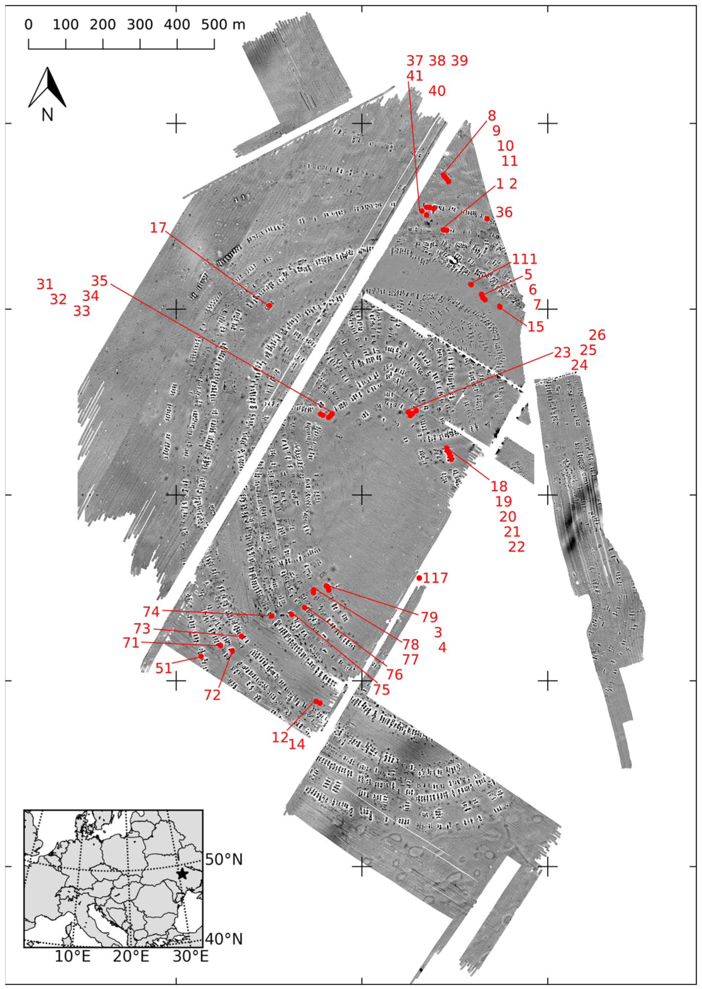
Magnetic map of the site Maidanetske (white: −10 nT, black +10 nT). The examined buildings and trenches are marked. Specifically, the three completely excavated buildings are house 44 (here, in trench no. 51), house 54 (here, marked with consecutive number no. 33), and the megastructure (here, in trench no. 111). In the lower left corner, the location of Maidanetske is marked with a star.

Different types of architectures are known through surveys and excavations: Thousands of domestic dwellings of the Tomashivka regional group show specific constructive characteristics and a high degree of standardization (Chernovol, 2012). Most striking are massive, originally uplifted platforms in the houses, consisting of wooden sub-constructions and partly thick covering layers of chaff-tempered and untempered clay. Relatively lightweight walls of the upper storage supported rounded roofs that can be identified in Chalcolithic house models (Shatilo, 2016). The houses show a very standardized internal division into mostly two and sometimes three rooms, as well as internal furnishing with ovens, installations, grinding stones, and numerous ceramic vessels preserved at the place of their use. ‘Standard houses’ with an anteroom and main room are distinguished from longer and rarer ‘extended houses’ with one additional chamber for workshops (cf. Figure 7).

Another category of buildings is the so-called ‘megastructures’, which are interpreted as communal facilities because of their highly visible positioning in the public space of the settlement (Burdo and Videiko, 2016; Chapman et al., 2016; Müller et al., 2016a; Ohlrau, 2015). In contrast to domestic dwellings, such buildings do not show an elevated platform but only a simple floor applied on the underlying terrain surface (Korvin-Piotrovskiy et al., 2016). Frequently, in the magnetic map of megastructures, the debris of relatively lightweight constructed external walls is particularly visible, while in contrast, the internal area either appears largely empty or shows varying masses of debris from collapsed walls.

The vast majority of houses in Tripolye settlements show traces of burning in varying intensity. In Maidanetske, almost 80% of the buildings are clearly burned, while the condition of the remaining ones is less clear. Findings of clearly burned domestic dwellings usually consist mainly of the highly fired and dropped-down platform. On top of this platform are found the following: daub remains of the internal wall, separating the anteroom and main room, foundation remains of an oven, a central clay installation, a podium on the longitudinal side, and sometimes storage bins (cf. Figure 7). In addition, there are grinding stones and larger quantities of ceramic vessels. Together with the overlying daub of the external wall, these remains form a dense package of highly magnetized materials.

Weak visible house remains that are usually classified as ‘partly burned’, ‘eroded’, ‘unburned’, or ‘possibly burned’ house remains represent the most frequent (20%) deviation from standard houses. Two such objects were excavated in Nebelivko. Indeed, they contained a normal amount of partly secondary burned pottery and some burned installations. However, very few and fragmented daub samples that were partly vitrified were unearthed (Вiдейко et al., 2015b). Based on these observations, the excavators interpret the features as remains of houses that consisted mainly of wood and only a low amount of daub. Assuming the deliberate character of the house burning, insufficient addition of fuel and the resulting lower burning temperatures were suggested as an alternative explanation (Chapman, 2017). Further scenarios take into account the character of these buildings as nonresidential storage buildings or as dwellings that were abandoned during the occupation of the settlement (Diachenko, 2016).

Methodological development and data acquisition

Interpretation concept for magnetic data of large settlements

The archeological investigation of a settlement with the dimension of Maidanetske needs an appropriate excavation design based on well-defined research questions. Taking the enormous size of the settlement into account, only very small excavation windows can be opened. Minimizing the size of the excavation areas is not only an aspect related to the research strategy but also a necessary condition for respecting heritage management guidelines and protecting the archeological archives.

The vast majority of houses need to be identified and classified on the basis of areal magnetic measurements alone. Whereas locating house remains on a magnetic map is straightforward, a joint effort combining geophysical computation with soil and find analyses is needed to perform a quantitative interpretation of the magnetic field data.

In this respect, we develop an approach allowing us to answer questions regarding (1) how the magnetized material associated with each house is spread out in depth and horizontally and (2) how much of this material is present.

Before discussing the details of the analysis procedure, we present an overview of its components and how they interconnect in this section. Because of its principal ambiguity, magnetic model development can only be performed under certain given preconditions. First, we explain the assumptions on which the novel interpretation approach is based, followed by an outline of the concept itself. Next, the methodical details for every step are described.

In the subsequent section ‘Numerical modeling of magnetic anomalies’, we investigate how different find categories contribute to generating magnetic field anomalies. We use the digitally documented spatial distribution of daub and pottery of a megastructure that was excavated in 2016. These data are converted into a magnetic subsurface model, for which synthetic magnetic data are computed. The comparison of the observed and modeled data illustrates the model quality, and the spatial correlation of each digitally documented find category is shown by the model itself.

Having identified the magnetically most significant material (which is daub in our case), we follow the interpretation scheme illustrated in Figure 2. It consists of the following steps:

Step1 – Identification of depth and thickness of the magnetized soil layer: given the magnetic field data, the depth and depth range of soil layer containing the magnetic material have to be identified by exemplary drillings and excavations. This information serves as a numerical constraint under which the distribution of the magnetized material is determined by a so-called inversion computation from the magnetic data. This process is necessary because the spatial distribution of magnetic material cannot be found from magnetic mapping alone, since the magnetic anomalies are ambiguous with respect to shape, depth, and volume-specific magnetization of subsurface materials. Alternatively to drilling and excavation, these depth constraints could also be gained through depth-sensitive geophysical methods if the depth functions of the respective physical soil parameters correlate with magnetization. In the present case, we can limit the magnetic layer to a specific depth range, which is justified by the excavations at the Cucuteni-Tripolyesites. These excavations showed that the remains of the buildings form a dense layer with a high fraction of daub in a specific depth range. The horizons above and beneath this archeological layer show a homogeneous solely induced magnetization and can therefore be neglected in the calculations.

Step 2 – Estimation of geological bias: since the procedure of mass determination relies on the applicability of a general, though location-specific, mass-magnetization relation (Step 3), an assessment of whether bias exists in the form of a spatial variability of potentially magnetic geological layers must be performed. To investigate this, daub samples, soils, and sediments were investigated considering their elemental composition and magnetic susceptibility. Since the source material of the daub is the local loess, the variability of the loess was also determined to enable a respective assessment.

Step 3 – Determination of magnetization map: using the depth information from Step 1, the areal distribution of magnetization is determined inside the magnetic layer from the magnetic survey data by an inversion. This process results in a map showing the magnetization distribution that is in accordance with the measured magnetic field strength.

Step 4 – Establishing a magnetization-mass relation: for converting the volume-specific magnetization determined in Step 3 into the mass of magnetized material, an empirical calibration curve is needed, which can then be applied to quantify the magnetic masses of unexcavated buildings. For determining a calibration curve, the excavation of key targets is needed, including a documentation of the archeological materials with respect to spatial distribution and weight. In the presented case, the masses of daub and pottery per square meter were weighed (cf. ‘excavation technique and daub documentation’) during the excavation of three buildings. From these data, an average calibration curve is computed that also allows us to numerically assess the uncertainties of the resulting mass estimates.

Step 5 – Determination of magnetized mass distribution: In the next step, the calibration curve of Step 4 is applied to the magnetization map determined in Step 3, resulting in a map of magnetized masses. This map can then be analyzed with respect to archeological criteria such as the bulk mass or the shape of house remains.

Figure 2.

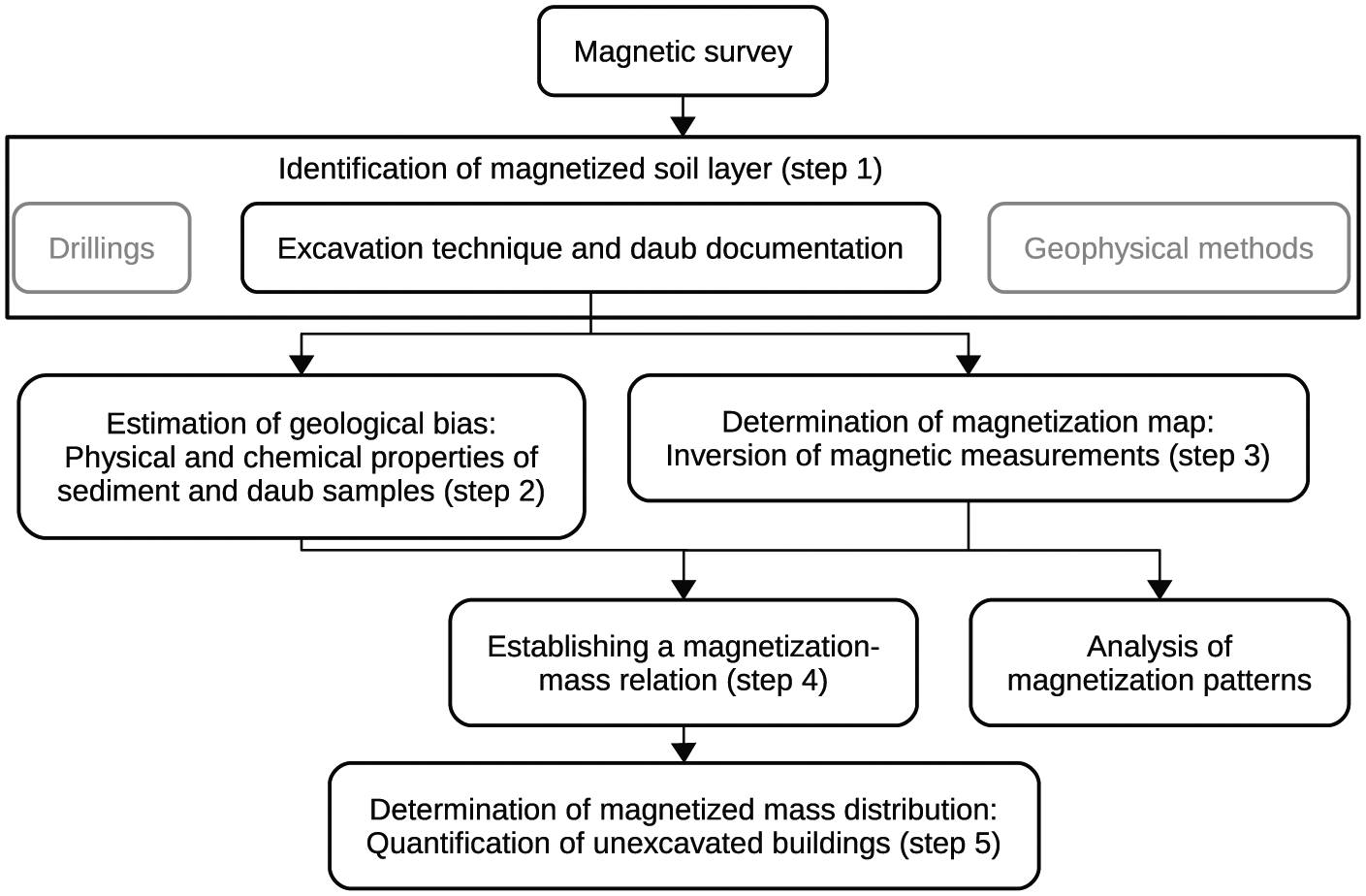
Flowchart of the novel interpretation scheme with Steps 1–5 (cf. ‘Methodological details’).

In sum, the magnetic map is transferred first into a map of magnetization and then into a map of masses of daub and pottery. This approach introduces new possibilities for the archeological interpretation of magnetic measurements at archeological sites with an almost uniform basement geology. The distribution of magnetization, respectively, the concentration of daub and pottery can be interpreted in terms of different internal layouts of buildings (cf. ‘Analysis of magnetization patterns’). The application of the outlined methodology to a whole settlement or even a complete area of settlements can reveal different types of buildings possibly related to ancient societal transformations. It may contribute to a better understanding of the settlement structure, to population estimations, and thus to calculation of the human impact on the forest steppe environment.

Magnetic survey

Since 2011, magnetic surveys have been conducted at the site Maidanetske using the FGM650 gradiometers by Sensys. Most of the total 185 ha has been surveyed in a motorized manner, with a sensor distance (crossline) of 25 cm and a sensor height of 35 cm. With a survey speed between 12 and 16 km/h and a sample rate of 20 readings per second, the inline point distance results in approximately 30 cm. Details of the processing can be found in Rassmann et al. (2016).

Excavation technique and daub documentation (Step 1)

For this study, the results from two completely excavated burned dwellings 44 and 54 (excavations in 2013 and 2014), of one burned megastructure (excavated in 2016), and of 23 small test trenches in the area of burned dwellings (excavated in 2013, 2014, and 2016) are available, which provide a clear picture of the stratigraphical variability in the settlement area (Müller and Videiko, 2016; Müller et al., 2017; Ohlrau, 2018). Additionally, other object categories such as pits, remains of pottery kilns, and ditches have been archeologically investigated in a systematic way.

After removal of the Chernozem top layer, the architectural remains (packages of daub and pottery) of dwellings and the megastructure were removed layer by layer. During this excavation process, the position and masses of archeological finds and daub were systematically documented with point coordinates and ordered in a grid of 1 ×1 m² cell sizes. The documentation of daub includes not only the recording of masses differentiated according to material properties but also registration and mapping of type, direction, and dimensions of wood negatives (Müller et al., 2017).

Physical and chemical properties of sediments and daub samples (Step 2)

The density of 33 samples (14 from the megastructure, 19 from house 44) was determined by dividing the dry weight of selected pieces (between 1 and 2.5 cm in diameter) by its volume (calculated via volume of replaced water). For 75 daub pieces (26 from the megastructure, 49 from house 44), the mass-specific magnetic susceptibility ( $κ$ ) was measured after homogenization < 2 mm following the procedure of Dearing (1999) using a Bartington MS2B susceptibility meter (resolution $2 \times 10^{- 6}$ SI, measuring range $1 - 9999 \times 10^{- 5}$ SI, systematic error 10%). Three samples of each piece were measured, and a standard sample (1% ${Fe}_{3} O_{4}$ ) was measured after each three measurements to check for device drift and to calibrate the results.

Analysis of the elemental composition of 92 daub pieces (38 from the megastructure, 53 from house 44) was carried out on a portable energy dispersive x-ray fluorescence spectroscopy (ped-xrf) device, namely, a Niton XL3t900-ed-XRF. The dried samples (one week at 35°C) were ground in a mortar and homogenized in an agate mill before measurements. For the measurements, He-flotation in the measurement chamber was used. The measurement mode was ‘mining-mode, Cu/Zn’, and the total measurement time was 300 s: main filter, 40 kV, 50 µA- 60 s; high filter, 50 kV, 40 µA- 60 s; low filter, 20 kB, 100 µA- 60 s; light filter 6 kV, 100 µA- 120 s. The semiquantitative results were converted into quantitative percentages per weight according to Dreibrodt et al. (2017). The mass-specific susceptibility and the total iron content of the loess and the soil that developed within that deposit were determined in 16 soil profiles (157 samples in total) at different parts of the settlement area in the same manner as described for the daub above.

Numerical modeling of magnetic anomalies

The terms ‘numerical modeling’ and ‘forward calculation’ describe the calculation of synthetic measurement data based on a numerical model of the subsurface in terms of physical parameters. In this case study, the given spatial distribution of the archeological finds is the basis to calculate the theoretically resulting anomalies of the vertical component of the magnetic field. We approximate the archeological structures by polygonal bodies, which allow calculation of the magnetic fields using the formula of Plouff (1976). The computations were performed with a Python code using the library ‘Fatiandoa Terra’ by Uieda et al. (2013). The total magnetization is assumed parallel to the magnetic field at the time of the survey according to the ‘International Geomagnetic Reference Field’ (IGRF) (Thébault et al., 2015). The magnetic field anomaly is calculated with unit magnetization. It represents a normalized anomaly that can be adjusted to the field data by multiplication with the actual magnetization magnitude.

Inversion of magnetic measurements (Step 3)

The inversion computation leading to the areal distribution of soil magnetization is based on fitting synthetic to measured magnetic data. To achieve this, we define the thickness and depth of the magnetic soil layer according to the depth and thickness of the daub layer as inferred from excavations and drillings. We assume that the observed magnetic anomalies are mainly caused by the magnetization of the burned clay, compared with which the magnetization of the surrounding unburned soil can be neglected. Additionally, we assume that the magnetization direction of the daub is parallel to the direction of the ambient earth’s magnetic field. Next, we divide the magnetic layer into regular grid cells with a given constant depth and thickness but unknown magnetization.

Each model cell $i$ is attributed an unknown magnetization $M_{i}$ , which contributes to the magnetic field anomaly. In our case, $M_{i}$ can be assumed to be scalar values because the direction of magnetization is assumed to be given. The linear superposition of the magnetic fields of all grid cells represents the anomalous magnetic field at the observation points $j$ . The relative field contribution of magnetized cell $i$ to the magnetic field observed at point $j$ is described by the elements $A_{j i}$ of matrix $A$ in Eq. (1). The synthetic data $d_{j}^{s y n}$ at point $j$ is accordingly expressed as

d_{j}^{s y n} = \sum_{i = 1}^{n} A_{j i} \cdot M_{i}

(1)

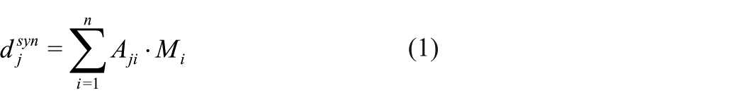
In this study, $d_{j}^{s y n}$ represents the difference in the vertical components of the magnetic field, as measured at the heights of the sensors of the differential magnetometer applied in the field. We computed the relative field strengths at positions $j$ of the magnetized cells at positions $i$ with the formula of Bhattacharyya (1964) (implemented in the Python library ‘Fatiando a Terra’ by Uieda et al., 2013). We applied the ambient magnetic field values according to the IGRF at the time of the magnetic survey (B = 49867.1 nT, I = 65.8918°, D = 6.6206°).

The cost function, which is minimized by the inversion computation, is

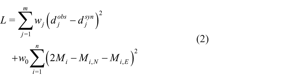
\begin{matrix} L = \sum_{j = 1}^{m} w_{j} {(d_{j}^{o b s} - d_{j}^{s y n})}^{2} \\ + w_{0} \sum_{i = 1}^{n} {(2 M_{i} - M_{i, N} - M_{i, E})}^{2} \end{matrix}

(2)

Here, the sum of the squared residuals between the observed $d_{j}^{o b s}$ and synthetic data are weighted with $w_{j} = 1$ . The second term represents a smoothness constraint, where $M_{i, N}$ and $M_{i, E}$ denote the northern and eastern neighbors of $M_{i}$ , respectively. This term is weighted with the constant $w_{0} = | \max (A_{j i}) |$ . The weight $w_{0}$ is dependent on the depth and thickness of the magnetized layer and varies for our examples between 1.3 and 5.0.

The $M_{i}$ values are determined through minimizing $L$ under the constraint $M_{i} > 0$ . The $M_{i}$ values have to be positive scalars because the direction of magnetization – parallel to the ambient magnetic field – is contained implicitly in the matrix elements $A_{j i}$ and because burned daub is not diamagnetic (diamagnetic materials would have negative $M_{i}$ values).

Computationally, we solved the minimization and inversion problem by applying the so-called subspace trust region interior reflective (STIR) algorithm (Branch et al., 1999), which is a well-established and robust method for nonlinear constrained and unconstrained optimization problems. In the first step, an initial estimate of the $M_{i}$ values is obtained by solving the problem in a least-squares sense without positivity constraints. Next, using these starting values, the STIR algorithm is applied in an iterative way, in which the constraints $M_{i} > 0$ are considered through Kuhn–Tucker conditions. Details of the method can be found in Coleman and Li (1996) and Branch et al. (1999). For the computations, we applied an open-source Python script (scipy.optimize.least_squares) of the scipy library (Jones et al., 2001–).

Establishing a magnetization-mass relation (Step 4)

To determine the masses of daub and pottery of unexcavated buildings, a relation between magnetization of the grid cells, determined through the inversion computation, and the masses of the causative magnetic material must be established. This relation can be derived from the excavations of the Maidanetske site (house 44, house 54, and megastructure), where the masses of daub and pottery have been documented per square meter. Under the assumption that density and volume-specific magnetization of the collected finds are almost constant, this relation is linear.

In principle, the relation can be determined by a bivariate regression between the daub masses, pottery masses, and magnetization of the grid cells. However, in all excavations, the found masses of daub were much higher than the pottery masses so that the regression coefficient of the pottery could not reliably be determined. Therefore, the masses of burned material were summed and treated as an entity.

Eq. (3) describes the linear relation between the mass of burned material $m_{A}$ and the mean magnitude of magnetization $| \bar{M} |$ in the volume $V$ of one grid cell

a_{1} \cdot m_{A} \cdot V^{- 1} + a_{2} = | \bar{M} |

(3)

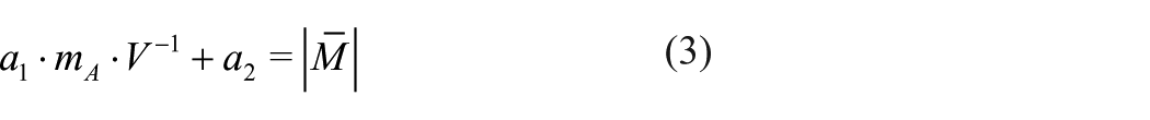
The coefficients $a_{1}$ and $a_{2}$ are determined by orthogonal distance regression (ODR) (e.g. Boggs and Rogers, 1990) because both the mass of burned material and magnetization are prone to statistical errors.

Since the regression coefficients $a_{1}^{(1)}$ , $a_{1}^{(2)}$ , and $a_{1}^{(3)}$ obtained for the three excavated buildings do not agree exactly, we use the middle of the interval

a_{1}^{⋆} = \frac{(a_{1}^{\max} + a_{1}^{\min})}{2}

(4)

as a representative value of $a_{1}$ , where $a_{1}^{\min}$ and $a_{1}^{\max}$ are the minimum and maximum of the determined $a_{1}^{(1)}$ , $a_{1}^{(2)}$ and $a_{1}^{(3)}$ . We use the extrema $a_{1}^{\max}$ and $a_{1}^{\min}$ as an estimate of the uncertainty of $a_{1}^{⋆}$ .

The application of Eq. (4) is motivated by the small number of only three excavations (‘samples’), from which no meaningful average and standard deviation of $a_{1}$ can be computed. With the chosen approach, we assume that the samples bound the possible interval of $a_{1}$ in the sense of a generalized Gaussian of order ∞ (box distribution) such as underlying the $a_{1}$ -norm. This normalized probability density function is centered at the midrange (4), and the uncertainty is given by half of the bandwidth. A more reliable value of $a_{2}$ can be obtained when data of more excavated houses are available.

The variable $a_{2}$ represents an average magnetization offset, which is independent of the recorded find masses. It is caused by the background magnetization of the soil enriched by small grains of daub and ceramics, too small to be collected. Since these values may be quite variable, we made no attempt to define a representative $a_{2}$ -value. Instead, the magnetization offset was determined independently for each investigated building by determining a representative magnetization value of the cells surrounding it.

For this purpose, the following procedure was developed and tested at the three example excavation sites:

The visibly magnetized area of each dwelling is circumscribed with a 2-m wide polygonal stripe.

A cumulative magnetization histogram is determined for the cells of this stripe.

The 75% mark is then used as the representative local $a_{2}$ -value.

The application of the approximate coefficient $a_{1}^{⋆}$ and local $a_{2}$ -value determined as described in the three example sites showed that the gathered find masses could be recovered with an accuracy of ±11%.

Quantification of burned masses of unexcavated buildings (Step 5)

The procedure described in the previous paragraph was exemplarily applied to 45 unexcavated houses, listed in Table 1. These houses were selected according to the following criteria:

Table 1.

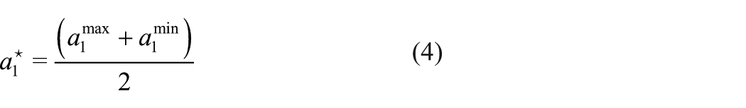
Information on examined buildings. The locations are given in Figure 1 with the ID. The buildings are divided into the categories burned (b), ‘unburned/eroded’ (u/e), and megastructure (m).

ID	Intercept $a_{2}$ (A/m)	Max. magnetization (A/m)	Mass (t)	Min. mass (t)	Max. mass (t)	Area (m²)	Mass/area (kg/m²)	Category	Trench	House ID	Contextual information/remarks
1	0.39	3.48	1.6	1.4	1.8	85.1	18.7	b	110	71	Burned floor but no platform, partly excavated 2016
2	0.02	0.25	0.1	0.1	0.1	57.6	1.6	u/e			Settlement 2
3	0.05	0.2	0.1	0	0.1	43.9	1.3	u/e			Settlement 2
4	0.09	0.34	0	0	0	44.4	0.8	u/e			Settlement 2
5	0.25	1.59	0.4	0.3	0.4	62.4	6.1	u/e			Settlement 1
6	0.23	1.98	0.6	0.6	0.7	89.3	7.1	u/e			Settlement 1
7	0.3	1.95	0.4	0.4	0.5	63.4	6.5	u/e			Settlement 1
8	0.38	1.16	0.1	0.1	0.1	48.1	2.2	u/e			Settlement 1
9	0.41	2.11	0.6	0.5	0.7	99.8	6.3	b			Settlement 1
10	0.36	4.13	0.8	0.7	0.9	92.5	8.2	b			Settlement 1
11	0.39	1.81	0.2	0.2	0.2	64.3	3.2	u/e			Settlement 1
12	0.15	0.44	0.1	0.1	0.1	61	2.1	u/e			Settlement 2
14	0.09	0.38	0.2	0.2	0.3	94	2.4	u/e			Settlement 2
15	0.33	3.56	1.7	1.5	1.9	219	7.6	m			Settlement 2, empty interior space
17	0.52	2.94	5.9	5.2	6.7	431.5	13.6	m			Settlement 2, interior space overbuild
18	0.24	1.34	0.6	0.5	0.7	69.3	8.3	b			Settlement 2
19	0.14	2.07	2.9	2.5	3.3	124	23.3	b			Settlement 2
20	0.02	1.04	0.9	0.8	1	80.4	11	b	96	66	Settlement 2
21	0	2.48	3.2	2.8	3.7	130.4	24.7	b	96	65	Settlement 2
22	0.2	3	6.8	6	7.8	166.3	41.1	b			Settlement 2
23	0.14	1.95	0.6	0.6	0.7	53.7	11.8	b			Settlement 2
24	0.25	3.63	1.6	1.4	1.8	66.5	23.5	b			Settlement 2
25	0.27	3.87	1.5	1.3	1.7	64.9	23.4	b			Settlement 2
26	0.22	1.16	0.2	0.2	0.3	54.3	4.2	b			Settlement 2
31	0.55	2.51	1.2	1	1.3	75.9	15.5	b			Settlement 2
32	0.51	3.76	3.2	2.8	3.7	94.6	33.7	b	91	58	Settlement 2
33	0.62	4.1	1.9	1.7	2.2	71.9	26.5	b	92	54	Settlement 2
34	0.65	2.67	0.6	0.5	0.7	71.6	8.7	b			Settlement 2
35	0.18	1.59	0.8	0.7	0.9	64.7	12.7	b			Settlement 2
36	0.33	2.8	1.4	1.2	1.6	64	21.5	b	103	70	Settlement 2
37	0.19	3.77	2.5	2.2	2.9	79.5	31.8	b	100	67	Settlement 2
38	0.16	1.53	0.3	0.3	0.4	41.2	7.8	u/e			Settlement 2
39	0.81	3.85	5.2	4.5	5.9	204.9	25.2	b			Settlement 2
40	0.24	2.82	1.3	1.1	1.4	73.2	17.1	b	99		Settlement 1
41	0.1	1.77	0.8	0.7	1	71.8	11.6	b			Settlement 1
51	0.46	5.06	3.9	3.4	4.4	110	35.2	b	51	44	Settlement 2
71	0.89	3.83	1	0.8	1.1	39	24.5	b	71	45	Settlement 2
72	0.68	3.7	1.5	1.3	1.7	85.8	16.9	b	72	46	Settlement 2
73	0.88	5.15	2	1.8	2.3	61.1	33.1	b	73	47+48	Settlement 2
74	0.46	3.48	2.6	2.3	3	137.3	18.8	b	74	49	Settlement 2
75	0.34	4.92	3.1	2.8	3.6	85.2	36.8	b	75	50	Settlement 2
76	0.6	3.99	2.1	1.8	2.4	72.8	28.4	b	76	51	Settlement 2
77	0.81	4.88	1.9	1.7	2.2	68.7	27.8	b	77	52	Settlement 2
79	0.14	2.74	2.4	2.1	2.7	108.2	22.1	b	79	53	Settlement 2
111	0.2	1.72	1.8	1.6	2	262.4	6.8	m	111		Settlement 2, interior space partly overbuild

The main selection criterion for the set of objects was the availability of either direct information on the depth range from test trenches, excavations and drilling cores, or the existence of depth information from adjacently located excavations or test trenches. Another intention was to test the method on a variety of different types of dwellings that were classified in the categories ‘burned’, ‘unburned/eroded’, and ‘megastructure’ as well as those belonging to different phases of the site.

Results

Before we start explaining the results obtained from magnetic mapping on the exemplary masses and mass distribution of houses, we focus on the laboratory measurements of the daub and sediment samples to show that no significant geological bias was observed.

Physical and chemical properties of sediments and daub samples

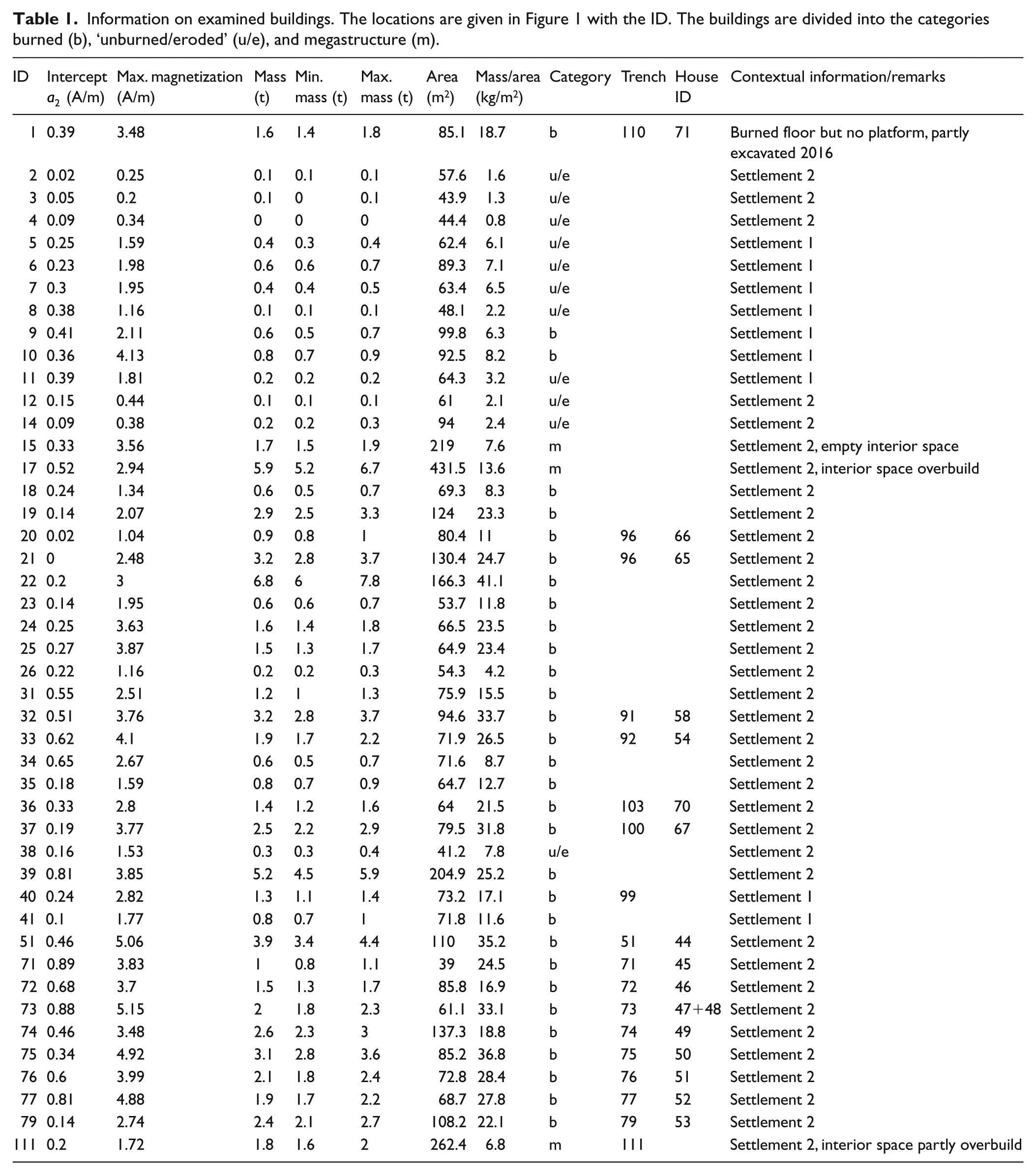
The medians of the densities (cf. Figure 3b) of daub pieces of house 44 and the megastructure were not significantly different with respect to their 25% and 75% quartile levels. The same applies to the medians of the mass-specific magnetic susceptibility (cf. Figure 3c). Moreover, as a main source of magnetism, the total iron content (cf. Figure 3a) of the daub samples does not differ significantly between the two objects. These findings are important because they also justify indirectly the assumption of homogeneity of daub magnetization underlying the interpretation procedure.

Figure 3.

Results of laboratory measurements. (a) Total iron content by weight, (b) density, and (c) mass-specific susceptibility of daub samples from the mega-structure and house 44. (d)–(h) Depth-dependent total iron content of different profiles. (i)–(m) Depth-dependent mass-specific susceptibility of different profiles. The locations of the profiles are given in Figure 1.

The total iron content (cf. Figure 3d–h) in the soils and sediments displays a mean of 2.28%. The measured range spans from a minimum of 1.94% by weight to a maximum of 2.86% by weight (whereas the latter is considered an outlier). Measurements of low-frequency mass-specific susceptibility on soil profiles through and beside houses and the megastructure are given in Figure 3i–m. They show little background variability in the Chernozem that overlays the cultural layer (approximately $100 \times 10^{- 8} m^{3} / kg$ ) with a peak in the depth of the archeo-deposits (approximately $200 \times 10^{- 8} m 3 / kg$ ). Note that in the profiles 76a, 77b, 78ac, and 110, the archeological record is reflected by higher susceptibility values.

Results of numerical modeling study

In this section, we verify the relative contributions of the different find categories to the magnetic patterns of houses by numerical modeling. The bases of this computation are the georeferenced finds of the megastructure, which are not the entirety of finds but can be considered as representative regarding the spatial frequency distribution and location of find categories within the building. Figure 4a shows the distribution of the single objects that have been digitally recorded for the find categories of daub from walls and floor and of pottery from the megastructure (cf. location: no. 111 in Figure 1, magnetic measurements: Figure 4f). Figure 4b–d shows the relative synthetic anomalies of these objects, Figure 4e the superposition of them. Comparing these with the measured data (Figure 4f), we arrive at the following conclusions.

Figure 4.

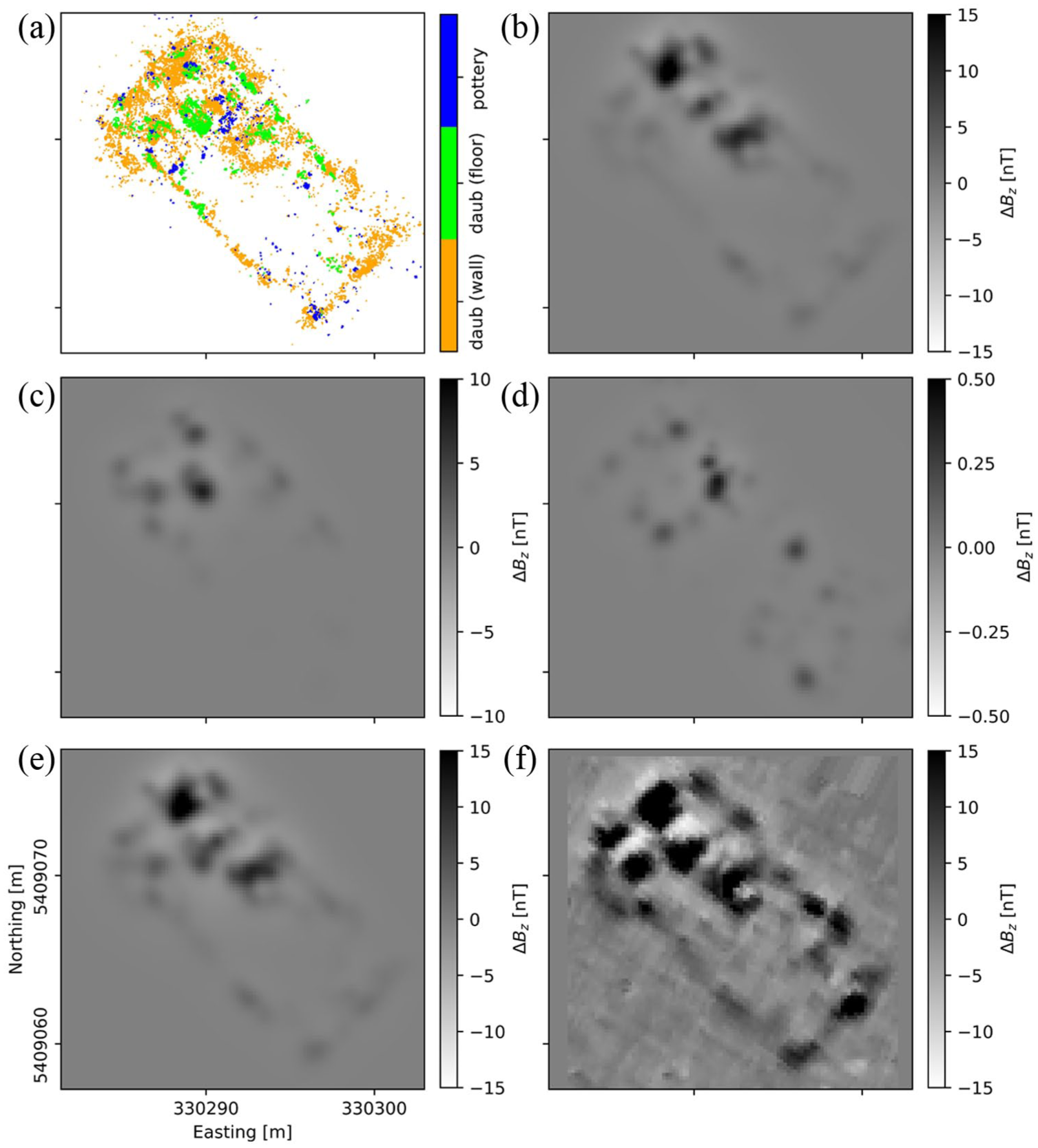
Exemplary building megastructure. (a) Digitally documented finds of the categories daub of walls, daub of floor and pottery, calculated magnetic anomalies for the find categories (b) daub of walls, (c) daub of floor, and (d) pottery. The bottom row shows a comparison of the sum of the (e) calculated anomalies and the (f) measured data.

The synthetic anomalies based on the daub assigned to walls (Figure 4b) resemble in their distribution the overall distribution of measured anomalies. Additionally, the location of local minima and maxima, especially in the northern quarter and the southern outline, correlate. However, the apsis-like shape in the western corner is calculated as a faint anomaly. The synthetic anomalies originating from the daub of the floor are shown in Figure 4c. They mainly appear in the northern half of the building, and the main maxima coincide with maxima in the measured data. In Figure 4d, the calculated anomalies of the pottery are depicted. The extrema of their amplitudes are approximately 50 times smaller than those of the daub from walls. Spatially, they are distributed over the complete area of the building with a gap in the central part.

Comparison of the synthetic with the measured data (Figure 4f) shows that the overall pattern of the measured magnetic anomalies is caused by the daub distribution and that the contribution of ceramics is only of minor importance.

Magnetization intensity of excavated buildings

The inversion yields magnetization maps (Figure 5b, e, and h) that show the areal distribution of magnetized soil matter in a more realistic way than the maps of magnetic field strengths (Figure 5a, d, and g). A comparison between the distribution of the digitally documented finds of the megastructure (Figure 4a) and the calculated magnetization (Figure 5h) shows that areas with increased magnetization coincide well with the location and frequency of finds. The modeling study of the previous paragraph indicated that the daub of the walls has the largest contribution to the magnetic anomalies. This result is confirmed by comparison of the inverted magnetization with the spatial density of the finds. It shows that the daub of the walls has the highest alignment with areas of increased magnetization.

Figure 5.

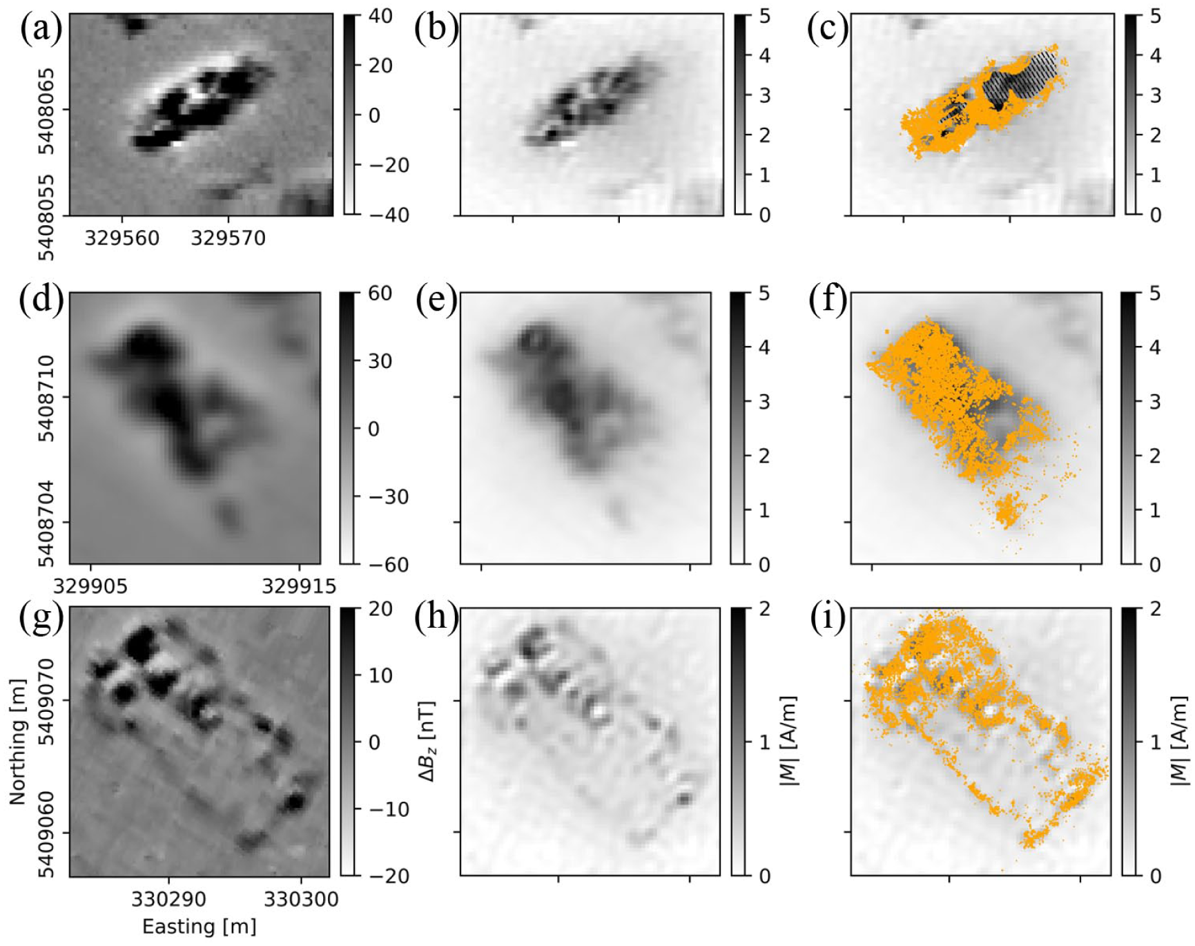
Comparison of measured magnetic data (left column: a, d, g), calculated magnetization (center: b, e, h), and documented daub in orange (right: c, f, i) for the three excavated buildings: house 44 (top row: a–c), house 54 (middle : d–f), and megastructure (bottom row: g–i). The hatched area in house 44 is disturbed because of illegal looting.

Relation between magnetization and magnetized masses

To transfer these results to the unexcavated houses, the relation between magnetization and magnetized masses was quantified by linear regression of the inverted magnetizations of the three excavated buildings and the recorded masses per excavation square. To determine the regression coefficients $a_{1}$ and $a_{2}$ of Eq. (3), the sum of the masses of pottery and daub are compared with the mean magnetization per excavation square (Figure 6). For the megastructure (Figure 6c), these are 392 squares, 200 for house 44 (Figure 6a) and 140 for house 54 (Figure 6b). In Figure 6, the squares with solely pottery are marked with light gray hexagons (⬡), those with solely daub with a gray triangle (▼) and those with both find categories with a point (•). The mass of pottery is small compared with the mass of daub and is equal or under 5% of the total mass for all three buildings. This difference makes a bivariate regression infeasible. The masses per volume range up to 0.2 t/m³ for the megastructure and up to 1 t/m³ (0.5 t/m³) for house 44 (54), and the mean magnetizations range up to 1.2 A/m and 4.5 A/m (4.0 A/m), respectively. The clear differences in the data ranges are also reflected in the different total masses of archeological material of 1.7 t for the megastructure and 4.4 t for house 44. The regression coefficients deduced for the three excavated buildings are given in Figure 6.

Figure 6.

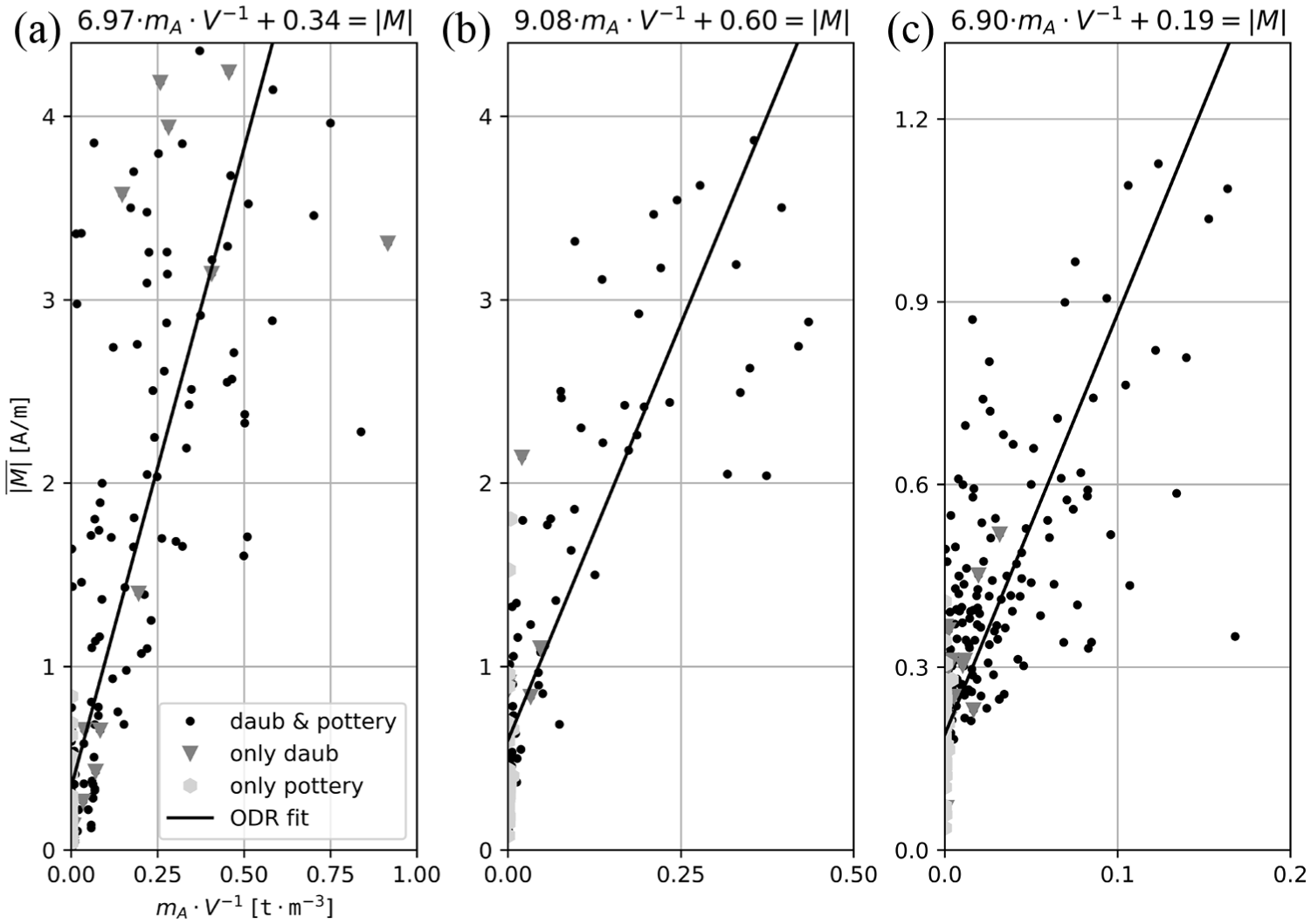
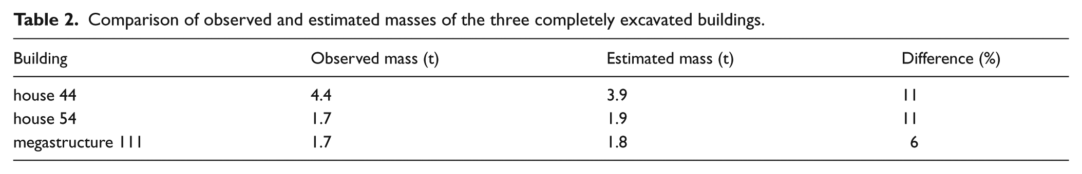
Mass-magnetization relation for (a) house 44, (b) house 54, and the (c) megastructure. The total masses of daub and pottery $m_{A}$ per volume $V$ are contrasted with the mean magnetization $| \bar{M} |$ .

In Table 2, the observed and estimated masses of the three excavated buildings are listed. They were calculated with the local coefficient $a_{2}$ (cf. Table 1) and $a_{1}^{⋆} = 8.0$ , resulting in a maximum difference of 11% between the measured and estimated masses.

Table 2.

Comparison of observed and estimated masses of the three completely excavated buildings.

Building	Observed mass (t)	Estimated mass (t)	Difference (%)
house 44	4.4	3.9	11
house 54	1.7	1.9	11
megastructure 111	1.7	1.8	6

Classification of houses from their magnetization patterns

To explore the archeological potential of the suggested interpretation concept, we applied it exemplarily to a total number of 45 dwellings. Three of them are megastructures, 12 are classified as ‘unburned/eroded’, and 30 as burned houses according to their appearance in the magnetic plan.

Comparing the patterns of the magnetization, different categories can be identified. The dwellings classified prior to the inversion as ‘unburned/eroded’ and megastructures remain in their own groups. In one megastructure (no. 15 in Figure 1), areas with high magnetization are found only for the exterior walls. In contrast, in the other two examples (nos 17 and 111 in Figure 1), the interior space also shows partly or complete areas with increased magnetization. Dwellings classified a priori as ‘unburned/eroded’ generally have low values of magnetization but show patches of increased magnetization not higher than 2 A/m (per inversion cell). Their diverse patterns make a further subcategorization infeasible.

After the inversion, the group of burned dwellings can be further subdivided based on patterns in the magnetization. Figure 7 shows exemplary buildings divided into three subgroups. For better comparison, the magnetization in each subfigure is scaled to its maximum, which is given in Table 1. Moreover, the houses are uniformly reoriented in the figure according to patterns described in the following. The largest subgroup (Figure 7, group 1) with 20 specimens shows a roughly rectangular area of increased magnetization, with one or two local maxima and a local minimum. Referring to the orientation of the standardized floor plan after Chernovol (2012), one local maximum is located at the backend. Moving from there to the front end, on the left side of the house, the local minimum can be seen in the central part. Further toward the front side, a local maximum is located. After that, the area of increased magnetization ends rather sharply. From there until the front end of the object, a zone of slightly increased magnetization commonly follows.

Figure 7.

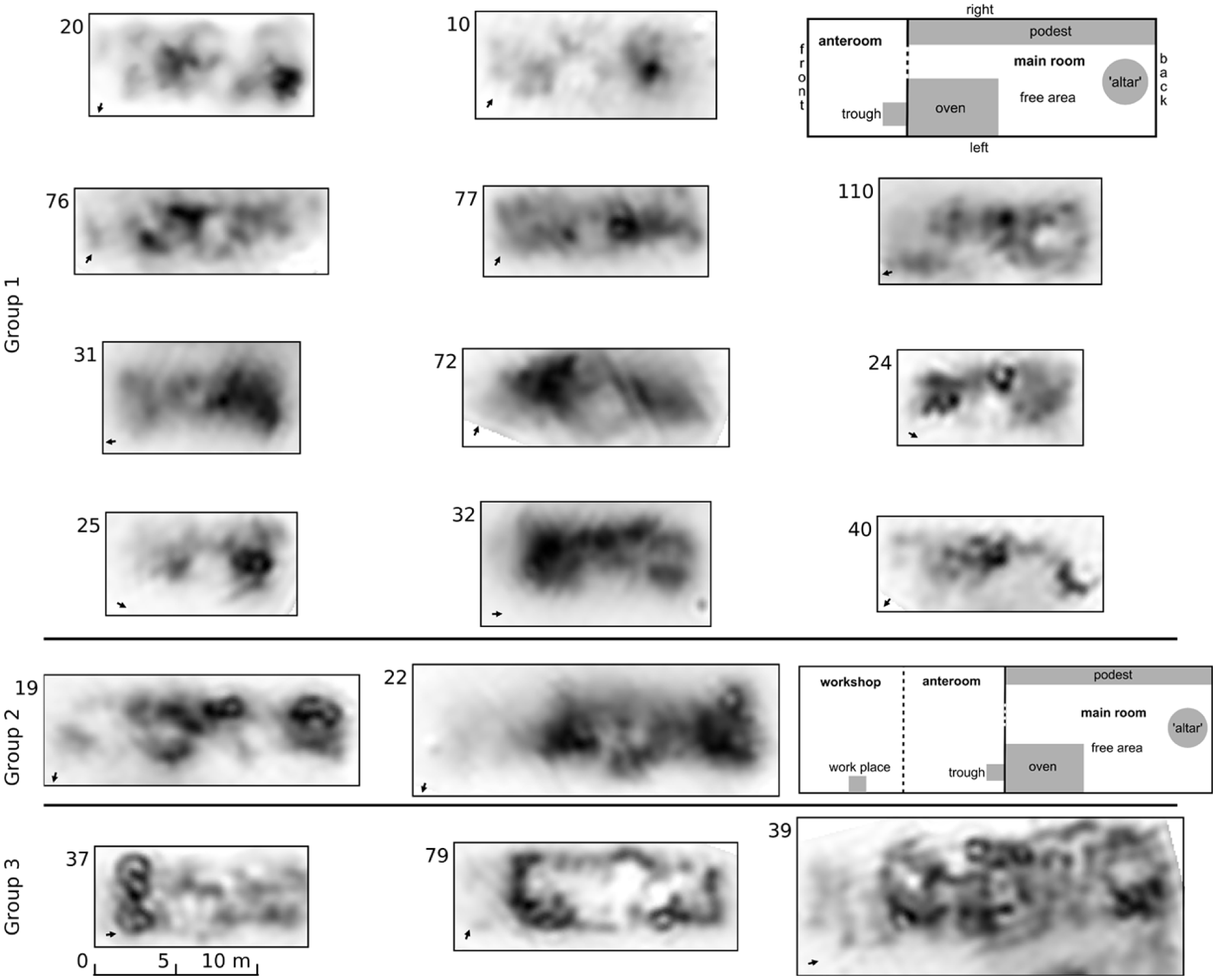
Magnetization maps (all to scale) of unexcavated buildings (white: 0 A/m, black: maximum magnetization). The maximum magnetization is given in Table 1. North is indicated in the lower left corner of each plot. For comparison, the schematic floor plans after Chernovol (2012) for the standard house (upper) and extended standard house (lower) are shown (not to scale). Group 1 are examples for the standard house, group 2 are examples for the extended standard house, and the examples of group 3 show individual patterns.

To test the regularities of the observed patterns, we additionally consider the location of the pit, which is usually associated with each house. For 15 of the 20 houses, the pit is situated on the backside. For the remaining five objects, the pit is on the opposite side. Moreover, there are five more houses with an insecure association to this group of houses.

A second group (Figure 7, group 2) is defined for houses that are larger than the houses of group 1. The group includes three specimens. The basic pattern is identical to the pattern of the houses of group 1. In comparison, however, the group 2 houses show a larger extent and a slightly increased magnetization at the front.

Three buildings are considered as a subgroup (Figure 7, group 3), showing nonuniform patterns in the magnetization. The left building (no. 37 in Figure 7) appears to show the magnetization pattern of the standard houses; however, at the front side, an area of increased magnetization is found. The central building no. 79 stands out because the areas of increased magnetization form its outlines, whereas the complete central part has low magnetizations. The third dwelling of this group (no. 39 in Figure 7) is the largest examined house.

Daub masses of unexcavated buildings

From the previous results, it can be concluded that the house masses, determined in the final step of the interpretation sequence, are basically daub masses. The results of the mass determination are summarized in Table 1. In Figure 8a, the masses determined for the 45 selected unexcavated houses are shown in comparison to the area of each dwelling. Figure 8b depicts the estimated total masses of the dwellings versus their total mass per area. 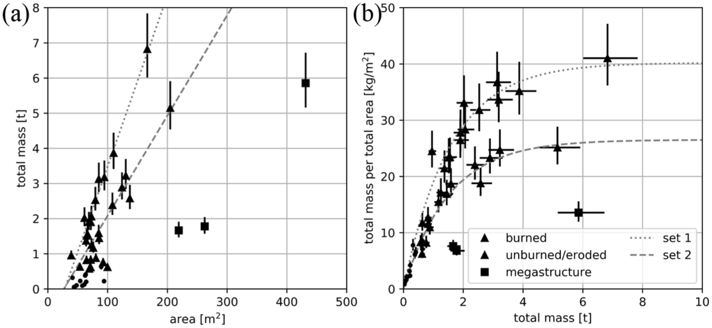The minimum and maximum of the regression coefficient ( $a_{1} \in [6.97, 9.08]$ ) have been used to calculate minimum and maximum estimates of the total mass (cf. Table 1) and consequently the total mass per total area. The masses range up to 7 t and the mass per area up to 41 kg/m². The house groups, classified from the magnetic map, can be identified also as groups in the mass diagrams. The ‘unburned/eroded’ buildings (•) have the lowest masses and are smaller than 100 m² (Figure 8a). In Figure 8b, they lie nearly on a straight line reaching from the origin to 0.6 t and 8 kg/m². The burned buildings ( $▲$ ) also approximately follow that line, up to values of 2 t and 20 kg/m².

Figure 8.

(a) Estimated total masses of examined buildings versus their area. (b) Estimated total mass per area versus total mass.

As shown in both graphs of Figure 8, the group of burned buildings separates apparently into two subsets, indicated tentatively by dashed and dotted gray lines. For the area-versus-mass plot, each subset follows a linear relation. Figure 8b shows the bulk mass per area of each building plotted versus its bulk mass. In this diagram, the tentative regression curves of the two subsets are nonlinear and appear to converge to a constant maximum value with increasing mass. Subset 1 consists of dwellings with an overall increased magnetization, whereas subset 2 consists of buildings showing only patches of increased magnetization. Compared with the houses, the megastructures ( $■$ ) are larger in size and have lower masses and lower masses per area.

Methodological discussion

In this section, we focus on the discussion of mainly methodological aspects. The archeological implications of the study are outlined in the next section.

How far does the presented interpretation approach differ from previously published magnetic interpretation methods?

During the past decades, a large number of studies targeting the quantitative interpretation of archeological magnetic prospection data have been published. The general problem of magnetic data inversion is the principal ambiguity of magnetic source models that can explain observed magnetic anomalies. Attempts have been made to reduce this ambiguity, for example, by applying weight functions regarding the magnetic field decay with depth (Argote et al., 2009), by making certain assumptions on the magnetic susceptibility (Eder-Hinterleitner et al., 1996; Herwanger et al., 2000; Neubauer and Eder-Hinterleitner, 1997), or by constraining positive and negative ranges of allowed susceptibility contrasts (Cheyney et al., 2015). Compared with these approaches, our computational scheme is quite simple, as it is basically a variant of the well-known equivalent-layer approach (e.g., Blakely, 1995), the realization of which is straightforward and merely a question of available computer power. Our approach can be applied here because we are able to impose quite strict constraints on depth and thickness of the major magnetic layer and to evaluate the results by drilling and excavations. The ‘new’ aspect of our approach lies therefore in the systemized coaction of geophysical, geoarcheological and archeological investigations, and not its single components.

What are the causes of the observed spatial variation of soil magnetization?

The presented magnetic interpretation is based on the assumption that the volume-specific magnetization of daub is almost homogeneous so that variations in magnetization can be translated into variation of magnetized mass. Alternatively, it might be considered that the soil from which the houses were constructed could have been heterogeneous from the beginning, especially in its iron content. In this regard, it has to be emphasized that the analysis of the physical and chemical properties of the daub pieces from houses and the megastructure did not show any statistically significant differences. This result implies that the measured properties cannot explain the variability observed in magnetization data. The total iron content of the sediments and soils at Maidanetske slightly varies from sample site to sample site, but the main differences, especially in maximum and minimum total iron content, are a result of a few outliers and are not statistically significant. Taking into account that the depth profiles (Figure 3) were taken from three different parts of the site, the results likely reflect a small-scale variability within the parent material (loess). A comparison of the total iron content of soil and sediment with that of the daub pieces clearly implies that the former was the material used by the Tripolye settlers to produce the latter. Thus, the variability of the parent material is also improbable to explain the observed variability within the magnetization data of the site.

How does the surrounding soil influence the determination of daub mass from magnetization?

Eq. (3) describes the relation between magnetized masses and magnetization. Regarding our idealized subsurface model, where nonzero magnetization is allowed only for the daub layer, an intercept a₂ of zero would be expected, whereas a nonzero intercept is observed. This intercept can be interpreted as the sum of the magnetizations of the hosting sediments and of all fragments of daub and pottery that were not recorded during the excavations. This interpretation is evident from investigations of excavation cells without any recorded daub or pottery in comparison to cells outside the buildings. The differences range from 0.01 A/m to 0.09 A/m, whereas differences would be close to zero if unrecorded fragments would not be present. At the present stage of investigation, this ‘diffuse’ magnetic background signal cannot be further interpreted. In future investigations, however, this aspect should be addressed by special sampling and onsite measurements.

Archeological implications of magnetization patterns and house masses

Analysis of magnetization patterns

The calculated magnetization enables a more distinct insight into the structures of the dwellings. This insight creates the potential for further examinations on the internal setup of the houses. For comparison, the floor plan of the ‘standard’ and ‘extended standard’ house by Chernovol (2012) is shown in Figure 7, besides the examples of calculated magnetization distributions. Additionally, in group 3, other constructive types of houses can also be identified that appear to be unrecorded in current classifications. In particular, house 79 resembles megastructures without an elevated platform because of its empty internal space.

For most inverted houses, the main room is characterized by two maxima and is distinguishable from the anteroom, which is characterized by a slightly increased magnetization at the front of the dwellings. Since several excavation reports (e.g. Kruts et al., 2001: 25; Kruts et al., 2013: 12, 15) note a thinner layer of daub for the anteroom (respectively ‘porch’), this indicates a difference in construction. This lighter type of construction can explain the relatively lower magnetizations compared with the main room. Moreover, for the majority of the dwellings, the area of slightly increased magnetization is on the opposite side than that of the pit associated with each dwelling. The pit was supposedly used to gather the construction material and is located at the backside of the house.

Despite their fuzziness, the displayed magnetization patterns resemble the floor plans, with the areas of increased magnetization belonging to the immovable interior elements. However, because of the fuzziness and the small number of excavated buildings, a clear assignment of spots of increased magnetization to the immovable interior remains insecure. For the excavated houses 44 and 54, no clear assignment can be made. However, for megastructure 15, the location of the central installation can be determined reliably.

Nevertheless, it is not clear if the local minimum of the magnetization distributions located mostly at the ‘left’ side of the buildings originates from the oven or the ‘free area’ toward the ‘backside’ of the building. In favor of the first possibility is the observation that in the excavated examples of the houses 44 and 54, the location of the oven coincides roughly with areas of lower magnetization. Additionally, it could be frequently shown by excavations that the oven was removed or destroyed. This observation gave rise to the assumption of ‘ritual demolitions’ of ovens during the process of house abandonment (Chernovol, 2012: 186; Круц, 2003: 76).

Facing the unsecure assignment of local maxima and immoveable interior elements, we need to take into account the possibility of factors for the location of the local maxima other than immovable interior components. For example, the collapsed material of the backend gable wall or the partition wall between the anteroom and main room might be the source of local maxima in the magnetization patterns. Moreover, both a microtopography and variations in the thickness of the daub layer can result in local extrema because of varying distances between the sensor and magnetized material. Furthermore, different positioning of parts of the immovable interior could also explain these deviations. Finally, the burning conditions are unknown and can vary not only among the buildings but also inside each building. This variation can influence both the formation of durable daub and the composition of (ferri)magnetic minerals.

Masses of unexcavated buildings

The masses of the excavated buildings are estimated with a maximum difference of 11%, which shows that the calculated masses are reliable estimates of the known masses. However, to our knowledge, no study is published aiming to quantify the mass of daub using geophysical methods.

The determined masses provide important new arguments for the discussion on houses with low magnetization that are currently frequently classified as potentially ’unburned’ or ’eroded’ dwellings. It is an important result that these objects contain low amounts of daub and do not represent completely unburned objects. According to our results of magnetic data interpretation, these remnants contain masses of daub and pottery in a range between 0.05 and 0.6 t at the lower end of the determined scale (cf. Figure 8/Table 1).

Similar results were obtained through the excavation of such a building place at the giant settlement Nebelivko (Burdo and Videiko, 2016: 107–110; Вiдейко et al., 2015b; Рудь, 2015). This feature was composed of small-sized, partly vesicular vitrified daub, one locally limited clay installation and larger quantities of pottery. Daub was distributed in a thin veil but also showed clusters at some places. Remains of installations such as the oven, the central installation and the podium, which are usually arranged on the top of the platform, were missing. The building contained a pottery assemblage of at least 19 vessels that showed clear traces of secondary firing. The vitrified daub and the secondary fired pottery might indicate that the firing happened at high temperatures.

We conclude that the labels ‘unburned’ or ‘eroded’ represent incorrect interpretations. Therefore, we suggest a specific expression ‘houses with a low amount of daub’. Far-reaching social and demographic interpretations of such buildings should be avoided as long as the structural reasons for the low masses of daub are not understood from the archeological side (e.g. Nebbia et al., 2018). Concerning the interpretation of buildings with low magnetization, different scenarios have already been discussed (e.g. Diachenko, 2016): The missing characteristic elements of dwellings such as ovens and podiums may indicate a nonresidential use. The low quantity of partly vitrified daub might, among other things, be explained through the use of only small amounts of clay to construct such buildings (Вiдейко et al., 2015b). Furthermore, the partial removal of daub from burned houses cannot be excluded, as large amounts of burned debris in pits show (e.g. Müller et al., 2017: 51–56). Due to the above described difficulties in the interpretation, it still remains very difficult to judge how such buildings should be interpreted with regard to demographic reconstructions. The considerable number of pits and ditches that are filled with daub indicate that the houses were not only burned at the end of Tripolye settlements but already during the use of the sites. Thus, it surely falls short to interpret houses with low magnetization as dwellings that were abandoned already during the life of a settlement.

A further tentative approach for an interpretation of the area-mass plot and the mass-mass per area plot is given in the following. After Chernovol (2012), the dwellings show a high degree of standardization, yet the area-mass plot indicates house sizes between 50 and 200 m². Idealizing the standardization and assuming identical burning conditions, a house of smallest size and mass should exist because a dwelling even smaller would be unusable. If all components of the building and the immovable inventory would scale proportionally with the size of the house, the relation between the size and the mass should be linear. Our data differ from this idealized image for several reasons: It is most likely that the burning conditions differ for each building and within each building because of variable movable and immovable interior elements. Furthermore, there are some variations in the floor plan of the houses that are possible, such as a second ‘altar’ (increase in total mass) in different locations of the building (Chernovol, 2012). Moreover, buildings with and without a platform, on which the buildings rests, exist (respectively, increase or decrease in total mass). It is rather unlikely that the constructional elements and the immovable interior scale proportional to the size of the building (e.g. thickness of walls). Additionally, the free, usable area might grow (decrease in total mass). Some excavations (Chernovol, 2012: 186; Круц, 2003: 76) showed that the oven was removed from the dwelling, resulting in a decrease in total magnetized mass. However, the size of the buildings is also an estimate based on the remains that produce the magnetic anomaly; therefore, an under- or overestimation is also possible. The anteroom is constructed in a lighter way (e.g. Kruts et al., 2001: 25; Kruts et al., 2013: 12,15), resulting in an uncertainty whether it is visible in the magnetic anomaly or magnetization map. The differences in the total mass for set 1 and set 2 (cf. Figure 8a) for dwellings of same size are of the order of a ton or more for buildings larger than 100 m². This difference seems to be too large to be explained by the existence or not of an oven. Summarizing, the tentative split in the two subsets resulting in different slopes for a linear relation between area and mass, most likely results from different types of construction and/or burning conditions. Thus, a general model of intentional house burning after abandonment suggested by Johnston et al. (2018) seems improbable. Either the inhabitants did not have equal access to wood to burn their houses, or the houses burned down under varying conditions. Since paleoecological results imply a proper wood delivery of the settlement throughout its inhabitation time (Dal Corso et al., this issue), the latter might be more probable.

In the mass per area versus total mass plot (Figure 8b), the two subsets of burned houses also become visible. While for masses higher than 4 t only a few examples exist, deliberate examination allows an asymptotic saturation curve to be observed. As a tentative interpretation, houses at the saturation level might be burned completely so that all building material is transformed into durable daub. The two different levels could then represent houses with and without a platform in the construction. For a more differentiated interpretation, a larger number of inverted houses ideally accompanied by additional examinations are needed, including measurements of the magnetic properties of daub and the determination of burning conditions.

Conclusion

Based on constraints from excavations and drillings, magnetic gradiometer measurements of the Chalcolithic Maidanetske settlement could be converted into an areal distribution of magnetization intensity by application of a rather simple inversion algorithm.

The resulting magnetization maps display the magnetized remains of the buildings in clearer images than the gradiometer measurements. This approach enables a distinct examination of patterns in the magnetization. A comparison with existing floor plans of excavated houses showed common structures, yet a clear identification of an immovable interior was not possible. However, in most cases, the orientation of the building could be identified. Comparison with the existing floor plans also showed that there might be buildings that do not fall into the existing classification.

Based on three excavated buildings, an empirical relation between the calculated magnetization and magnetized masses was found and applied to determine the masses of unexcavated buildings from magnetization maps. Based on test computations for excavated buildings, the accuracy of the derived masses is of the order of approximately ±10%. Masses of up to 0.6 t of daub are determined for buildings that were initially classified as ‘unburned/eroded’. Hence, rephrasing as ‘houses with a low amount of daub’ is suggested. Houses with higher masses can be grouped into two subsets if their ground areas are considered. These subsets might be a result of different burning conditions or construction types.

The interpretation scheme can be applied directly without modification to sites where the magnetic sources are confined to one distinct soil layer of approximately constant depth and thickness. If the thickness or depth of these layers varies significantly, site-specific modifications need to be incorporated, for example, using interpolated depths and thicknesses based on a densified grid of drillings.

The application of the novel interpretation scheme to the complete settlement can form the basis for a profound statistical analysis, including cluster analysis, of the size, mass and relative location of the buildings. Our tentative archeological interpretation can then be reevaluated, and the analysis of the settlement as a whole will lead to an improved understanding of settlement structure, population estimations and human impact on the forest steppe environment.

Footnotes

Acknowledgements

The authors thank the two anonymous reviewers for their constructive critical comments that helped to improve the paper.

Funding

The author(s) disclosed receipt of the following financial support for the research, authorship, and/or publication of this article: We are grateful to the Deutsche Forschungsgemeinschaft (DFG, German Research Foundation - Projektnummer 2901391021 – SFB 1266) for funding the presented research.

ORCID iDs

Natalie Pickartz

René Ohlrau

References

Argote

Tejero

Chávez

et al. (2009) 3D modelling of magnetic data from an archaeological site in North-Western Tlaxcala state, Mexico. Journal of Archaeological Science 36(8): 1661–1671.

Bhattacharyya

(1964) Magnetic anomalies due to prism-shaped bodies with arbitrary polarization. Geophysics 29(4): 517–531.

Blakely

(1995) Potential Theory in Gravity and Magnetic Applications. Cambridge; New York: Cambridge University Press.

Boggs

Rogers

(1990) Orthogonal distance regression. In: Brown

Fuller

(eds) Statistical Analysis of Measurement Error Models and Applications: Proceedings of the AMS-IMS-SIAM Joint Summer Research Conference Held June 10–16, 1989. Providence, RI: The American Mathematical Society, pp. 186–194.

Branch

Coleman

(1999) A subspace, interior, and conjugate gradient method for large-scale bound-constrained minimization problems. SIAM Journal on Scientific Computing 21(1): 1–23.

Burdo

Videiko

(2016) Nebelivka: From magnetic prospection to new features of mega-sites. In: Müller

Rassmann

Videiko

(eds) Trypillia Mega-Sites and European Prehistory 4100–3400 BCE. London; New York: Routledge, pp. 95–116.

Chapman

(2017) The standard model, the maximalists and the minimalists: New interpretations of Trypillia Mega-Sites. Journal of World Prehistory 30(3): 221–237.

Chapman

Gaydarska

(2016) Low-density urbanism: The case of Trypillia group of Ukraine. In: Fernández-Götz

Krause

(eds) Eurasia at the Down of History. Urbanization and Social Change. New York: Cambridge University Press, pp. 81–105.

Chapman

Gaydarska

Hale

(2016) Nebelivka: Assembly houses, ditches, and social structure. In: Müller

Rassmann

Videiko

(eds) Trypillia Mega-Sites and European Prehistory 4100–3400. London; New York: Routledge, pp.117–131.

10.

Chapman

Videiko

Hale

et al. (2014) The second phase of the Trypillia mega-site methodological revolution: A new research agenda. European Journal of Archaeology 17(3): 369–406.

11.

Chernovol

(2012) Houses of the Tomashovskaya local group. In: Menotti

Korvin-Piotrovskiy

(eds) The Tripolye Culture Giant-Settlements in Ukraine. Formation, Development and Decline. Oxford:Oxbow Books, pp.183–209.

12.

Cheyney

Fishwick

Hill

et al. (2015) Successful adaptation of three-dimensional inversion methodologies for archaeological-scale, total-field magnetic data sets. Geophysical Journal International 202(2): 1271–1288.

13.

Coleman

(1996) An interior trust region approach for nonlinear minimization subject to bounds. SIAM Journal on Optimization 6(2): 418–445.

14.

Dal Corso

Hamer

Hofmann

et al. (this issue) Modelling landscape transformation at the Chalcolithic Tripolye mega-site of Maidanetske (Ukraine): Wood demand and availability. The Holocene.

15.

Dal Corso

Out

Ohlrau

et al. (2018) Where are the cereals? Contribution of phytolith analysis to the study of subsistence economy at the Trypillia site Maidanetske (ca. 3900–3650 BCE), Central Ukraine. Journal of Arid Environments 157: 137–148.

16.

Dearing

(1999) Environmental magnetic susceptibility: using the Bartington MS2 system. 2nd ed. Oxford: Bartington Instruments.

17.

Diachenko

(2016) Demography reloaded. In: Müller

Rassmann

Videiko

(eds) Trypilla Mega-Sites and European Prehistory 4100–3400 BCE (Themes in Contemporary Archaeology). London; New York: Routledge, pp. 181–193.

18.

Dreibrodt

Furholt

Hofmann

et al. (2017) P-ed-XRF-geochemical signatures of a 7300 year old linear band pottery house ditch fill at Vráble-Ve’lké Lehemby, Slovakia-House inhabitation and post-depositional processes. Quaternary International 438 (Part B): 131–143.

19.

Eder-Hinterleitner

Neubauer

Melichar

(1996) Reconstruction of archaeological structures using magnetic prospection. Analecta Praehistorica Leidensia 28(2): 131–137.

20.

Fassbinder

(2015) Seeing beneath the farmland, steppe and desert soil: Magnetic prospecting and soil magnetism. Journal of Archaeological Science 56: 85–95.

21.

Gaffney

(2008) Detecting trends in the prediction of the buried past: A review of geophysical techniques in archaeology. Archaeometry 50(2): 313–336.

22.

Herwanger

Maurer

Green

et al. (2000) 3-D inversions of magnetic gradiometer data in archeological prospecting: Possibilities and limitations. Geophysics 65(3): 849–860.

23.

Johnston

Diachenko

Gaydarska

et al. (2018) The experimental building, burning and excavation of a two-storey Trypillia house. PAST (Newsletter of the Prehistoric Society) 89: 13–15.

24.

Jones

Oliphant

Peterson

et al. (2001–) SciPy: Open source scientific tools for Python. Available at: http://www.scipy.org/ (accessed 23 November 2018).

25.

Kirleis

Dal Corso

(2016) Trypillian subsistence economy: Animal and plant exploitation. In: Müller

Rassmann

Videiko

(eds) Trypillia Mega-Sites and European Prehistory 4100–3400 BCE. London; New York: Routledge, pp. 195–205.

26.

Korvin-Piotrovskiy

Hofmann

Rassmann

et al. (2016) Pottery kilns in Trypillian settlements. Tracing the division of labour and the social organisation of Copper Age communities. In: Müller

Rassmann

Videiko

(eds) Trypillia Mega-Sites and European Prehistory 4100–3400 BCE (Themes in Contemporary Archaeology). London; New York: Routledge, pp. 221–252.

27.

Kruts

Korvin-Piotrovskiy

Chabanyuk

et al. (2013) Taliank–Settlement-Giant of the Tripolian Culture. Investigations in 2012. Kiev: Institute of Archaeology of the National Academy of Science of Ukraine.

28.

Kruts

Korvin-Piotrovskiy

Rizhov

(2001) Talianki – Settlement Giant of the Tripolian Culture. Investigations in 2001. Kiev: Institute of Archaeology of the National Academy of Science of Ukraine.

29.

Linford

(2006) The application of geophysical methods to archaeological prospection. Reports on Progress in Physics 69(7): 2205–2257.

30.

Menotti

Korvin-Piotrovskiy

(2012) The Tripolye Culture Giant-Settlements in Ukraine: Formation, Development and Decline. Oxford: Oxbow Books.

31.

Müller

Videiko

(2016) New facts of a mega-site. In: Müller

Rassmann

Videiko

(eds) Trypillia Mega-Sites and European Prehistory 4100–3400 BCE. London; New York: Routledge, pp. 71–93.

32.

Müller

Hofmann

Ohlrau

(2016a) From domestic households to mega-structures: Proto-urbanism? In: Müller

Rassmann

Videiko

(eds) Trypillia Mega-Sites and European Prehistory 4100–3400 BCE. London; New York: Routledge, pp. 253–268.

33.

Müller

Rassmann

Videiko

(2016b) Trypilla Mega-Sites and European Prehistory 4100–3400 BCE. London; New York: Routledge.

34.

Müller

Hofmann

Brandtstätter

et al. (2016c) Chronology and demography: How many people lived in a mega-site? In: Müller

Rassmann

Videiko

(eds) Trypillia Mega-Sites and European Prehistory 4100–3400 BCE. London; New York: Routledge, pp. 133–170.

35.

Müller

Hofmann

Kirleis

et al. (2017) Maidanetske 2013: New Excavations at a Trypilia Mega-Site. Bonn: Habelt, R.

36.

Müller

Hofmann

Ohlrau

et al. (2018) The social constitution and political organisiation of Tripolye mega-sites: Hierarchy and balance. In: Meller

Gronenborn

Risch

(eds) Surplus without the State – Political Forms in Prehistory: 10Th Archaeological Conference of Central Germany October 19–21, 2017 in Halle (Saale). Halle (Saale): Landesamt für Denkmalpflege und Archäologie Sachsen Anhalt – Landesmuseum für Vorgeschichte, pp. 247–260.

37.

Nebbia

Gaydarska

Millard

et al. (2018) The making of chalcolithic assembly places: Trypillia megasites as materialized consensus among equal strangers? World Archaeology 50(1): 41–61.

38.

Neubauer

Eder-Hinterleitner

(1997) 3D-interpretation of postprocessed archaeological magnetic prospection data. Archaeological Prospection 4(4): 191–205.

39.

Ohlrau

(2015) Trypillia Großsiedlungen – Geomagnetische Prospektion und architektursoziologische Perspektiven. Journal of Neolithic Archaeology 17: 17–99.

40.

Ohlrau

(2018) Maidanets’ke. Development and decline of a Trypillian mega-site in Central Ukraine. PhD Thesis, Christian-Albrechts-Universität zu Kiel.

41.

Plouff

(1976) Gravity and magnetic fields of polygonal prisms and application to magnetic terrain corrections. Geophysics 41(4): 727–741.

42.

Rassmann

Korvin-Piotrovskiy

Videiko

et al. (2016) The new challenge for site plans and geophysics: Revealing the settlement structure of giant settlements by means of geomagnetic survey. In: Müller

Rassmann

Videiko

(eds) Trypillia Mega-Sites and European Prehistory 4100–3400 BCE. London; New York: Routledge, pp. 29–54.

43.

Rassmann

Ohlrau

Hofmann

et al. (2014) High precision Tripolye settlement plans, demographic estimations and settlement organization. Journal of Neolithic Archaeology 16: 96–134.

44.

Shatilo

(2016) Roofs of Tripolian houses. Reconstruction: Sources and problems. In: Preoteasa

Ciprian-Dorin

(eds) Cucuteni Culture within the European Neo-Eneolithic Context. Proceedings of the International Colloqium ‘Cucuteni 130’ 15–17 October 2014, Pietra Neamț, Romania. in Memoriam Dr. Dan Monah. in Memoriam Dr. Gheorghe Dumitroaia. Pietra Neamț:Editura Constantin Matasă, pp.725–740.

45.

Shatilo

(2017) Ornaments and signs on the sledge models from Talianki (Excavation 2012) – Art decor or a source of information? In: International Symposium ‘From Symbols to Signs. Signs, Symbols, Rituals in Sanctuaries’ (eds CE

Ursu

Poruciuc

Lazarovici

), Suceava, 9–11 September 2016, pp. 177–185. Suceava: Editura Karl. A. Romstorfer.

46.

Thébault

Finlay

Beggan

et al. (2015) International geomagnetic reference field: The 12th generation. Earth, Planets and Space 67(1): 67–79.

47.

Uieda

Oliveira

Barbosa

VCF

Jr (2013) Modeling the earth with Fatiando a Terra. In: Proceedings of the 12th Python in Science Conference (eds van der Walt

Millman

Huff

), Austin, TX, 24–29 June, pp.96–103. Available at: http://conference.scipy.org/proceedings/scipy2013/html/pdfs/uieda.pdf.

48.

Videiko

Rassmann

(2016) Research on different scales: 120 years of Trypillian large sites research. In: Müller

Rassmann

Videiko

(eds) Trypillia Mega-Sites and European Prehistory 4100–3400 BCE. London; New York: Routledge, pp.17–28.

49.

Вiдейко

МЮ

Мюллєр

Бурдо

НБ

et al. (2015a) Дослiдження у централнiй частинi Майданецького. Археологiя 1: 71–78.

50.

Вiдейко

МЮ

Чепмэн

Дж

Бурдо

НБ

et al. (2015b) Комплексные исследования оборонительных сооружений, производственных комплексов и остатков построек на трипольском поселении у села Небелевка.Stratum Plus 2: 147–170.

51.

Дудкiн

ВП

(2007) Магнiтометричнi дослiдження поселень трипiльської цивiлiзацiї. In: Кот

Вiдейко

(eds) Трипiльська Культура. Пошуки. Вiдкриття. Свiтовий Контекст. Киïв: Спадщина ЛТД, pp.57–70.

52.

Дудкин

ВП

(1978) Геофизическаяразведкакрупныхтрипольскихпоселений. InГенингВФ(ed.) Использование методов естественных наук в археологии.Киев:Наукова думка, pp.35–45.

53.

Журавльов

ОП

(2008) Тваринництво та мисливство у трипiльських племен на територiї України. Київ: Нацiонáльна акадéмiя наýк України. Iнститут археологiї.

54.

Кошелев

ИН

(2004) Памятники трипольской культуры (по данным магнитной разведки). Киев: Самиздат.

55.

Круц

ВА

(2003) Трипольские площадки -результат ри туального сожжения домов. In: Корвин-Пиотровский

АГ

Круц

ВА

Рижов

СМ

(eds.) Трипiльськi поселення-гiганти. Материали мiжнародної конференцiї. Tripolian Settlements-Giant. The international symposium materials. Київ: Корвин Пресс, pp. 74–76.

56.

Рудь

(2015) Дослiдження залишкiв жител на розкопi 5 поселення Небелiвка. In: Вiдейко

М Ю

Чапман

Дж

Козир

I А

(eds.) На схiднiй межi Старої Європи. Матерiали мiжнародної наукової конференцiї, Кiровоград, Небелiвка, 12–14 травня. Кiрово град, pp. 26–28.

57.

Шишкiн

КВ

(1985) Планування трипiльських поселень за даними аерофотозйомки. Археологiя 52: 72–76.

58.

Шмаглий

НМ

ВидейкоЮ

(2005) Майданецкое трипольский протогород. Киев: Национальная Академия Наук Украины Институт Археологии.

Deciphering archeological contexts from the magnetic map: Determination of daub distribution and mass of Chalcolithic house remains

Abstract

Keywords

Introduction

Tripolye megasites and the site Maidanetske

Methodological development and data acquisition

Interpretation concept for magnetic data of large settlements

Magnetic survey

Excavation technique and daub documentation (Step 1)

Physical and chemical properties of sediments and daub samples (Step 2)

Numerical modeling of magnetic anomalies

Inversion of magnetic measurements (Step 3)

Establishing a magnetization-mass relation (Step 4)

Quantification of burned masses of unexcavated buildings (Step 5)

Results

Physical and chemical properties of sediments and daub samples

Results of numerical modeling study

Magnetization intensity of excavated buildings

Relation between magnetization and magnetized masses

Classification of houses from their magnetization patterns

Daub masses of unexcavated buildings

Methodological discussion

How far does the presented interpretation approach differ from previously published magnetic interpretation methods?

What are the causes of the observed spatial variation of soil magnetization?

How does the surrounding soil influence the determination of daub mass from magnetization?

Archeological implications of magnetization patterns and house masses

Analysis of magnetization patterns

Masses of unexcavated buildings

Conclusion

Footnotes

Acknowledgements

Funding

ORCID iDs

References