
Abstract
Farming practice in the first period of the southern Scandinavian Neolithic (Early Neolithic I, Funnel Beaker Culture, 3950–3500 cal. BC) is not well understood. Despite the presence of the first farmers and their domesticated plants and animals, little evidence of profound changes to the landscape such as widespread deforestation has emerged from this crucial early period. Bone collagen dietary stable isotope ratios of wild herbivores from southern Scandinavia are here analysed in order to determine the expected range of dietary variation across the landscape. Coupled with previously published isotope data, differences in dietary variation between wild and domestic species indicate strong human influence on the choice and creation of feeding environments for cattle. In context with palynological and zooarchaeological data, we demonstrate that a human-built agricultural environment was present from the outset of farming in the region, and such a pattern is consistent with the process by which expansion agriculture moves into previously unfarmed regions.
Introduction
Southern Scandinavia represents one of the last European Neolithization events, in which domestic plants and animals appear concurrently with cultural change from the late Mesolithic Ertebølle culture (EBK, 5400–3950 cal. BC) to the early Neolithic Funnel Beaker Culture (EN, TRB, 3950–3300 cal. BC). The first 500–700 years of the Neolithic (ENI 3950–3500 cal. BC, ENII 3500–3300 cal. BC) in this region has long been described as a period of transition (Price and Noe-Nygaard, 2009; Zvelebil and Rowley-Conwy, 1984), but it is clear that by the end of the EN, farming was entrenched and had permanently altered the landscape. In this paper, we use the concept of expansion agriculture in conjunction with stable isotope data from wild herbivores to illustrate the character of early cattle (Bos taurus) husbandry. In particular, we use isotopic data from these cattle to demonstrate the immediate modification of the natural environment for farming. In so doing, we examine the case for immigrant farmers bringing agricultural lifeways to a previously unfarmed region. We argue that these immigrants brought entrenched ideas of how farming should be performed through the alteration of the natural environment.
To do this, we present both a review of the palynological data in the late Mesolithic and Neolithic and a review of the zooarchaeological data, and we integrate these with models of expansion agriculture. We combine this with new and previously published carbon- and nitrogen-stable isotopic data deriving from herbivore bone collagen to place cattle within the created and natural environment. Early domestic cattle show some overlap with Ertebølle and early Neolithic herbivores from a number of sites in southern Scandinavia, but they also show an overall pattern of variability contrary to what is expected for herbivores in natural Scandinavian environments. This indicates that the cattle were raised in open landscapes in part created by human activity. Forests and their resources were not widely utilized in this early period. To put these data in context, we discuss the period, synonymous with the EN, in which agriculture moves from a technology new to the region to a mature mode of food production that is archaeologically visible. This process probably was the result of the first farmers relying on a small-scale integrated regime of pastoralism and cereal cultivation in natural and created open environments characterized by small-scale clearance of the forests. Results serve to clarify the development of the Neolithic within the region’s landscape.
Expansion agriculture, land-cover change and farmers in the landscape
Expansion agriculture is the process by which farming moves into an unfarmed landscape and alters that landscape (Foley et al., 2005; Mustard et al., 2004). Agricultural expansion into previously unfarmed areas follows a predictable course during which the landscape undergoes a series of profound changes. Some changes are large scale and some are small scale. Any analysis focusing only on broad patterns or conversely only on local patterns will miss parts of the whole picture. Such a difference of scale is not only geographic but also temporal. If too long or too short a period is focused upon, then important trends have the potential to be overlooked. In true expansion agriculture, a group of individuals embracing and skilled in a fully agriculture-based subsistence strategy move into an ‘untouched’ landscape, gradually alter its composition and reduce the prevalence of natural cover (Foley et al., 2005; Mustard et al., 2004). The speed at which this happens and the character of the resulting land-use pattern depend on a number of factors, including numbers of individuals involved, the particular environmental setting and participation in modern market economies.
The land cover of landscapes can generally be classified into Undisturbed, Frontier, Agricultural/Managed and Urbanized/Industrialized (Mustard et al., 2004). Others have described similar patterns of land-use transitions (Foley et al., 2005) in context with the importance of agriculture in subsistence and its effect on original forest cover of a region. At first, the undisturbed land cover is characterized by little human use and natural disturbance. Next, frontier landscapes start to show changes, albeit on a small scale, from their natural state owing to human activity. Furthermore, agricultural or managed landscapes are those in which human activity has become the main factor causing change and consistency. Of importance is the speed at which one type of land cover moves to another, whether or not this occurs, and the individual setting of each particular case. Six case studies from numerous regions of the world show that the change from Frontier to Agricultural/Managed land cover can happen as fast as a few decades or can take as long as a thousand years (Mustard et al., 2004), predicated mostly on factors such as number of expansion agriculturalists, the local environment and others.
While modelled for modern world-systems, such frameworks may offer a complimentary view for understanding how agriculture matured within southern Scandinavia. Neolithization in this region has long been described as a process (Zvelebil, 1986; Zvelebil and Rowley-Conwy, 1984) proceeding from the integration of domestic plants and animals to a pre-existing economy at a very low frequency (Availability Phase) to a rapid increase in the integration of agricultural production into subsistence economies (Substitution Phase) to full-blown dominance of agricultural production in the economy. Of course, such a procession assumes a degree of integration of agriculture into pre-existing hunter-gatherer subsistence strategy, which implies a degree of indigenous adoption of agriculture in a secondary context.
Early farmers in southern Scandinavia
The first farming in southern Scandinavia is usually considered to have been small scale (see Rowley-Conwy, 2004; Sørensen, 2014). Shifting or slash-and-burn agriculture, involving clearing, burning and short-term cultivation followed by a new clearing elsewhere, was originally argued to be the likely early Neolithic method of cultivation. Even small-scale cultivation would have involved considerable areas of clearance, with old clearings regenerating and turning back into forest (Boserup, 1965; Iversen, 1949). Slash and burn is, however, no longer seen as the likely method. Small long-lasting clearances are more likely (Lüning, 2000; Rowley-Conwy, 1981, 2003; Sherratt, 1980), similar to the earliest farmers in central Europe (Bogaard, 2004) from whom the first Scandinavian farmers came. Pollen spectra from burial mounds claimed to indicate slash and burn cultivation (Andersen, 1988, 1992) are in fact equally compatible with fixed fields (Rowley-Conwy, 2004: 93).
Small-scale farming of this type may initially affect only a small percentage of the forested landscape. There is remarkably little visible palynological evidence of widespread forest clearance for agriculture in the ENI. This is related to a number of factors, some of which have nothing to do with human activity and, in some cases, are almost certainly biases in the archaeological record. A good example is the variable distance the pollen of different species travels (Berglund, 1985), meaning that less-common taxa could be over-represented if their pollen travels farther. Therefore, herbivores have the potential to provide a different view of the landscape, as each individual animal lived its life in a particular environment or combination of environments. As such, it is possible to establish the expected range of variation of local environments that were present across the landscape through investigating the browsing and grazing behaviour of deer through bone collagen isotope analysis of carbon and nitrogen.
Previous research lacks discussion of domestic animals within the available settlement pattern data (e.g. settlement versus catching sites) and within context of the natural environment (e.g. Noe-Nygaard et al., 2005). However, evidence for a human-built environment for agriculture still remains elusive until visible in the palynological record in the ENII and MN (younger than 3300 cal. BC). Our aims are therefore threefold: (1) establish the expected range and character of variation in wild herbivores about the transition and (2) characterize the feeding environments of domestic species. In doing so, we will (3) determine through comparison whether it is possible to conclusively determine whether there are built agricultural environments in the ENI by pinpointing the presence of domesticated species in such environments. We expect that if cattle are being raised in natural environments, their diets and range of variation will approximate those of the deer.
The flora
In many ways, the early Neolithic landscape in southern Scandinavia was dynamic. The body of research concerning the vegetation in the late Mesolithic and the early and middle Neolithic documents change, some of which, almost certainly human induced, occurred across the landscape (Andersen, 1992, 1993; Berglund, 1969, 1985; Göransson, 1988; Regnell and Sjögren, 2006). From the outset, however, it must be acknowledged that the palynological record is incomplete and much of the available data are removed geographically from sites yielding substantial faunal material. While problematic, such is the state of affairs, and awaiting further work in this regard, the use of such data stands as the only option in discussions of this type.
In very general terms, the unaltered Mesolithic mixed forest landscape included predominantly alder, oak, lime, ash, elm and hazel, with little or no suggestion of human modification (Andersen, 1993; Lageråds, 2008). Starting about the Atlantic-Subboreal transition, a series of changes in the landscape began. The first change was the ‘classical’ elm (Ulmus sp.) decline, a marked and widespread reduction in the number of elm trees across much of northern Europe and southern Scandinavia (Regnell and Sjögren, 2006). This event is largely coincident with the start of the Neolithic (Göransson, 1988; Troels-Smith, 1960) and absolute dating places this event in the period of around 4000 to 3800 cal. BC (Andersen, 1993). However, this date is variable by location and often more restricted chronologically. At Ageröd Mosse, Scania, Sweden, for example, the decline is dated to several decades around 3770 cal. BC (Skog and Regnéll, 1995) while at Bökebjerg, also in Scania around 40 km away, the decline is dated somewhat earlier, at ca. 3980 cal. BC (Regnell et al., 1995). Therefore, the picture is one of variation in timing of the decline, even at sites close to each other.
The elm decline was formerly attributed to human clearance of the forest or a by-product of human forest exploitation (Troels-Smith, 1953, 1960). It is now generally considered to have been the result of multiple factors, including change in the climate and elm disease, although the possibility of a human role is not completely excluded (Göransson, 1988; Regnell and Sjögren, 2006). In the 1940s, Iversen (1949) proposed that the series of changes that followed the elm decline represented the period in which the landscape was occupied and cleared by Neolithic groups, a process which he termed the ‘landnam’. In eastern Denmark, this is characterized by a birch peak which follows the elm decline and is coincident with the EN, which in turn is followed by a hazel peak by the Middle Neolithic (MN TRB, 3300–2300 cal. BC). All of the post-elm decline changes in forest composition were interpreted in this case as being the result of intentional human modification of the landscape for agricultural activities (Andersen, 1993).
Demonstrating intentionality in human impact on the environment is difficult but there is some evidence to this effect in the ENI. One characteristic pattern on the local level is that the floral succession may represent the regeneration of forest for grazing of cattle on the quickly growing secondary invading plants (Andersen, 1998). In one case, soils from within ENI Volling vessels from and contemporary with the Bjørnsholm long-barrow and shell midden yielded a substantial proportion of pollen which had been deformed through heating, indicating a recent burning episode (Andersen, 1992). This was interpreted as a deliberate burning to encourage the growth of secondary flora.
There is heterogeneity, however, in terms of actual dominant species and the rate and character of changes by location. This makes it difficult to speak of the floral composition of the landscape in anything more than general terms. For example, forest vegetation at Tågerup in the earliest Neolithic in Scania consisted primarily of oak, elm and lime trees (Regnell and Sjögren, 2006) but at Brunnshög, near the modern city Lund, in Scania, while the hardwood-dominated forest remained, there was evidence of some small-scale clearance and regeneration in the form of herb and pine growth (Lageråds, 2008). The pollen data in most areas of southern Scandinavia record a similar pattern of vegetative cover in the EN (Andersen, 1993; Berglund, 1969; Regnell and Sjögren, 2006), but it is important to emphasize the inconsistent nature of the available record across the landscape.
By the end of the EN, however, signs of forest clearance become clearer and more common. These include many secondary plants such as grasses and herbs and a general opening up of the environment (Lageråds, 2008). By the MN, the landscape had changed markedly yet again, with unambiguous evidence of human modification of the landscape observed for the first time (Regnell and Sjögren, 2006). It is at this point that the region can be considered ‘fully’ Neolithic.
The overall impression of the change in the flora from the Mesolithic to the MN is one of gradual movement towards a more open and modified landscape from the earliest Neolithic into the middle Neolithic. In the EN, and especially the ENI, there is little unambiguous evidence at all of human effects on the flora of the region. The evidence available seems to indicate human disturbance in the form of forest clearings followed by regeneration. Then, starting in the ENII and moving into the MN, clearance and a significant human impact become evident. Of importance though is the impression that landscape clearance for grazing and agriculture is very local in its character: different localities show the impact of these activities to a different degree.
The fauna
There are two general classes of faunal assemblage in the ENI: those dominated by domestic species and those dominated by wild species. These correspond to the two general types of site that are found in the period: hunting camps with predominantly wild fauna and residential sites with an almost entirely domestic fauna (Johansen, 2006). Examples of hunting camp faunal assemblages include those from Havnø, Norsminde, Bjørnsholm and Muldbjerg (Andersen, 1991; Bratlund, 1993; Gron, 2013; Noe-Nygaard, 1995); residential assemblages include sites such as Havnelev (Koch, 1998). Nowhere is this dichotomy more evident than in eastern Sweden at the sites Anneberg and Skumparberget: Anneberg is almost completely dominated by seal remains, while Skumparberget has almost entirely domesticated animals. This is despite the fact that both sites belong to the Funnel Beaker culture are contemporary and are geographically close to one another (Hallgren, 2008; Segerberg, 1999). However, the picture is not always so clear, as there are also sites that may be communal centres that were not strictly residential, but instead visited from time to time. Almhov is an example of this type (Rudebeck, 2010), whose assemblage may present a biased picture as domestic animal herds may not have been resident at the site (Gron et al., 2015).
Faunal assemblages are best described as small and poorly preserved. They often remain unpublished and offer in most cases only a glimpse into early Neolithic animal-based subsistence. Some of the largest assemblages are those from the aforementioned Almhov and Muldbjerg (Noe-Nygaard, 1995; Rudebeck, 2010), but even these yielded fewer than 2000 bones determinable to species. Some material is well preserved, such as the material from the Store Åmose bogs in central Zealand (Gotfredsen, 1998), but the fauna from these sites is dominated by wild species with only a few domestic specimens and do not permit a widespread view of Neolithic life. Much more typical EN assemblages are those from the shell midden sites on Jutland, Denmark (Norsminde, Bjørnsholm, Havnø), which usually number only in the hundreds of highly fragmented specimens identifiable to species (Andersen, 1991; Bratlund, 1993; Gron, 2013).
The small samples, the high degree of fragmentation and poor preservation preclude a number of different types of zooarchaeological analyses such as age-at-death profiles, repeated stress indicators, sex determination and any other of a number of lines of evidence that usually can be used for understanding the role of cattle in a prehistoric economy. While some data of these types are available from the largest TRB assemblages (Rudebeck, 2010), such information is rare and equivocal. The role of the domestic fauna in the EN economy is thus largely invisible in the zooarchaeological record. At present, zooarchaeology can only contribute in a limited fashion to understandings of ENI farming practice.
Despite these problems, there is widespread evidence of the presence of cattle from about ca. 4000 cal. BC, and their appearance is synchronous within the resolution of the radiocarbon curve (Noe-Nygaard et al., 2005; Price and Noe-Nygaard, 2009). Any earlier dates are highly controversial, but accepted dates indicate introduction on a wide geographic scale and largely coincident with the earliest uncontested dates coming from far-flung reaches of the TRB (Price and Noe-Nygaard, 2009; Rowley-Conwy, 2013). Simply, cattle are a key feature of early TRB agriculture.
Previous herbivore stable isotope research
As in many world regions, the published archaeological stable isotope data from southern Scandinavia are dominated by samples deriving from humans (see Fischer et al., 2007). These data have reinforced the long-held notion (Tauber, 1981) that there is a marked and immediate shift to terrestrial foods from the start of the Neolithic. Data for animals, however, are much more limited. Particularly lacking are data from wild herbivores to serve as an isotopic baseline for interpreting the diets of domestic species. Such a comparison is valid because cattle are grazers, and deer are both browsers and grazers depending on the species and local environmental conditions.
However, some previous data are available. In the Åmosen lacustrine bog system in Zealand, Denmark, Noe-Nygaard (1995) analysed a number of archaeological and modern herbivore bone collagen samples for their carbon stable isotope values. Her data from modern deer from known environments demonstrated that the openness of browsing environments does affect isotope values in deer in this region. A later study of both aurochs and early cattle (Noe-Nygaard et al., 2005) documented change in browsing environments through the Holocene in both carbon and nitrogen isotopes. Fischer et al. (2007) focused primarily on human diets and dogs as proxies, but included some faunal samples as a baseline. Finally, Craig et al. (2006) analysed several deer samples from the Jutland shell middens at Bjørnsholm and Norsminde, and Ritchie et al. (2013) published several isotope measurements on wild fauna from Asnæs Havnemark, an Ertebølle site on the coast of western Zealand.
Most relevantly, Noe-Nygaard et al. (2005) used previous data (Noe-Nygaard, 1995) to argue that the earliest cows in Scandinavia were brought into open, coastal grasslands, because of the higher δ13C values of the domestic cattle in comparison with deer from the sites Muldbjerg and Præstelyng in central Zealand. While the cattle samples were predominantly from Zealand, several were from elsewhere in southern Scandinavia, including Jutland and northern Germany. While we are aware of further analyses currently being performed, the general impression is that a much more comprehensive view across the region is required for understanding similarity or difference in browsing environments of early domestic cattle and deer.
Materials and methods: Carbon and nitrogen in bone collagen
Bone collagen samples were selected from a number of late Mesolithic and early Neolithic archaeological sites in southern Scandinavia (Table 1; Figure 1). Samples were taken from several transitional Mesolithic–early Neolithic sites as well as a few purely early Neolithic or late Mesolithic localities (Table 1; Figure 1). Most specimens are indirectly dated, with the greatest confidence context or site age given. Mesolithic sites are included in order to ensure that the sample of deer contains animals that were browsing in all available natural environments. Several taxa were sampled: red deer (Cervus elaphus), roe deer (Capreolus capreolus), domestic cattle and undifferentiated bovids (Bos sp.), which could be either domestic cattle or wild aurochs (Bos primigenius). Cattle from Scania were all considered domestic on the grounds that aurochs were absent in the region by the late Mesolithic (Aaris-Sørensen, 1999; Ekström, 1993). Domestic cattle from Jutland were only assigned to taxon if diagnostic measurements could be taken (Degerbøl and Fredskild, 1970). Otherwise, they were classified as Bos sp., given the possibility that they could be aurochs. Limited numbers of domestic ovicaprids (Capra sp./Ovis sp.) were also sampled but could not be differentiated to genus on morphological grounds.
Sites, samples and isotope data from southern Scandinavia (struck-through samples omitted from discussion based on their atomic C:N).
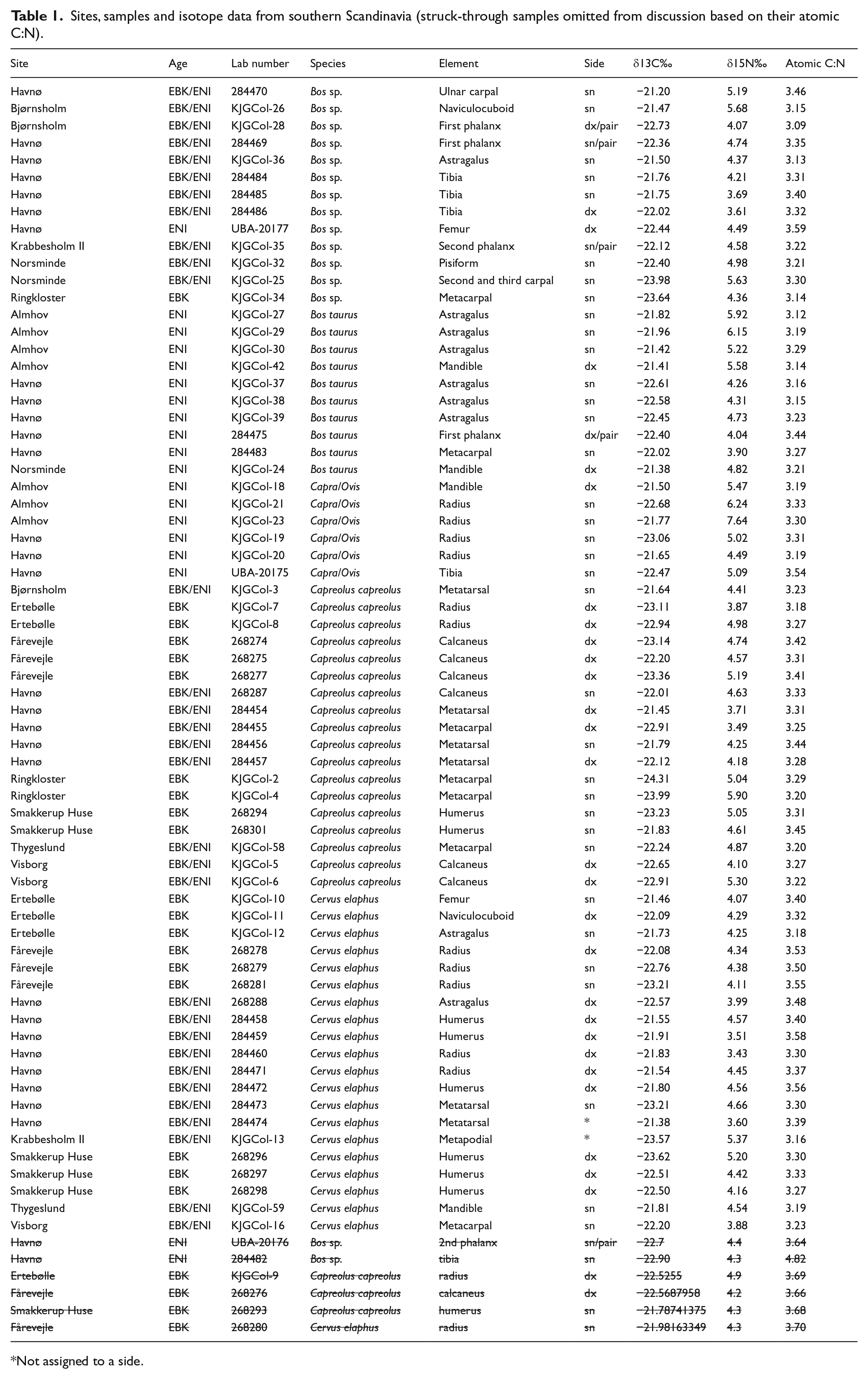
Not assigned to a side.
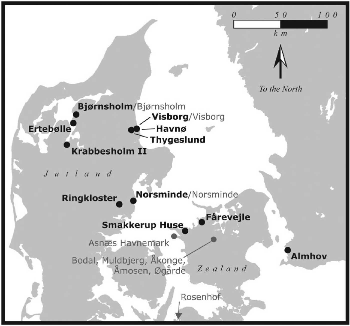
Map of sites from which isotope samples were selected (bold site names indicate material analysed in this study, while grey site names indicate data from the literature).
Wherever possible, a Minimum Number of Individuals (MNI) (Casteel and Grayson, 1977)-based sampling approach was taken at each site. However, in many cases, this simply was not possible, as much of the material derives from shell middens characterized by high fragmentation. To mitigate the possibility of occasional accidental sampling from different elements from the same dead animal, a number of archaeological sites were sampled, and if possible remains from different features were selected. Several solely Mesolithic sites were included to ensure that the observed dietary values of wild species not the result of already-present human modification of the landscape.
Bone was first cleaned of surface contamination using a diamond-tipped dental rotary drill. Some minor variation of collagen extraction method (e.g. coarse grinding of the bone versus coarse chips of bone being used) was introduced by the standard protocols of different laboratories being applied. In this case, preparation work was undertaken at Copenhagen University’s Department of Geography and Geology, Durham University’s Department of Archaeology and at the CHRONO Centre at Queen’s University Belfast. Nevertheless, all collagen purification followed standard extraction methodology (Ambrose and DeNiro, 1986; Brown et al., 1988; DeNiro, 1985; Longin, 1971). Samples were analysed at the University of Waterloo’s Stable Isotope Facility and the University of Bradford’s Archaeological Stable Isotope facility and a few at the CHRONO Centre at Queen’s University Belfast. All laboratories strictly adhere to rigorous international quality control guidelines through the application of international reference standards. Only data with atomic carbon to nitrogen ratios in the range 2.9–3.6, indicating low probability of diagenesis (DeNiro, 1985), are interpreted. Maximum analytical error reported among the three labs was 0.25‰ for δ13C and 0.3‰ for δ15N, well within the reported range of variation in the data.
Results: Carbon and nitrogen in bone collagen
In all, 67 isotope measurements from southern Scandinavia had acceptable atomic ratios of carbon to nitrogen and therefore had no indications of diagenesis (Table 1) (DeNiro, 1985), while six were excluded as they were outside the acceptable range.The range of variation within the data generated in this study is shown in Table 2. Lowest δ13C variation is among the domestic cattle, at 1.23‰, with the highest variation among the roe deer. Red deer are intermediate. The Bos sp. which could not be determined to species also show a range of variation above 2‰, unsurprising given that this category likely contains forest-dwelling aurochs as well as domestic cattle. Similarly, the ovicaprids have a range of δ13C values higher than the cattle, probably stemming from the inclusion in the sample of both sheep and goats, animals that consume different types of vegetative foods. The range of variation in δ15N values is more uniform across taxa, with only ovicaprids showing a markedly larger range of variation than the other taxa.
The variation within the data (all values in ‰).
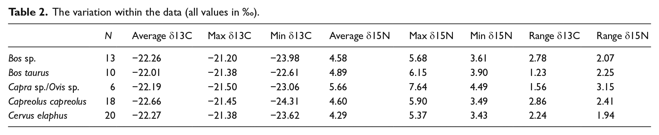
It is difficult to interpret the Bos sp. that could not be attributed to either cattle or aurochs. The same is true for the ovicaprids. This difficulty lies in the potential for vastly different feeding behaviours among these species. Cattle feed on what is provided to them or on what is available in the areas in which they are grazed. There likely could be wide variation in these source environments for foods. Conversely, aurochs were deep forest creatures (Van Vuure, 2005). Therefore, it is unwise to interpret the undistinguished Bos sp. specimens except to note that a wide degree of variation is seen among these specimens. Similarly, the ovicaprids display a large range of variation. It is also difficult to interpret these data because the inherent behavioural differences in feeding behaviour and regimes of domestic sheep and goats cannot be assessed without taxonomic certainty between the species. This is compounded by the small sample size. Furthermore, depending on whether these animals were raised for fibre, milk or meat, their diets may have differed. It is for these reasons that we will not further interpret the ovicaprid data, save to say that the spread of variation in all individuals does approximate the general trend seen in the cattle. Thus, as δ13C increases, so does δ15N.
Selecting only cattle samples dating to the ENI (AMS dated samples with complete ranges between 4000 and 3500 cal. BC selected from Noe-Nygaard et al. (2005) and Fischer et al. (2007) and using published EBK and EN deer values (Craig et al., 2006; Fischer et al., 2007; Ritchie et al., 2013) in conjunction with the new data from this study, it becomes possible to place the cattle in their Neolithic environment. It is of vital importance to have as large a comparative sample as possible in order to place early Neolithic cattle husbandry in the landscape. In total, 106 isotope measurements are displayed in Figure 2 from the sites in Figure 1; this combines our data with 39 previously published data points from the earlier studies (Craig et al., 2006; Fischer et al., 2007; Noe-Nygaard et al., 2005; Ritchie et al., 2013) all of which are rounded to the nearest second decimal place for plotting and statistics. Some further isotope values of wild herbivores from this region have been published (Eriksson and Lidén, 2002; Hede, 2005; Noe-Nygaard, 1995; Richter and Noe-Nygaard, 2003), but they are not included as they report either δ13C alone without δ15N or samples were very few in number.
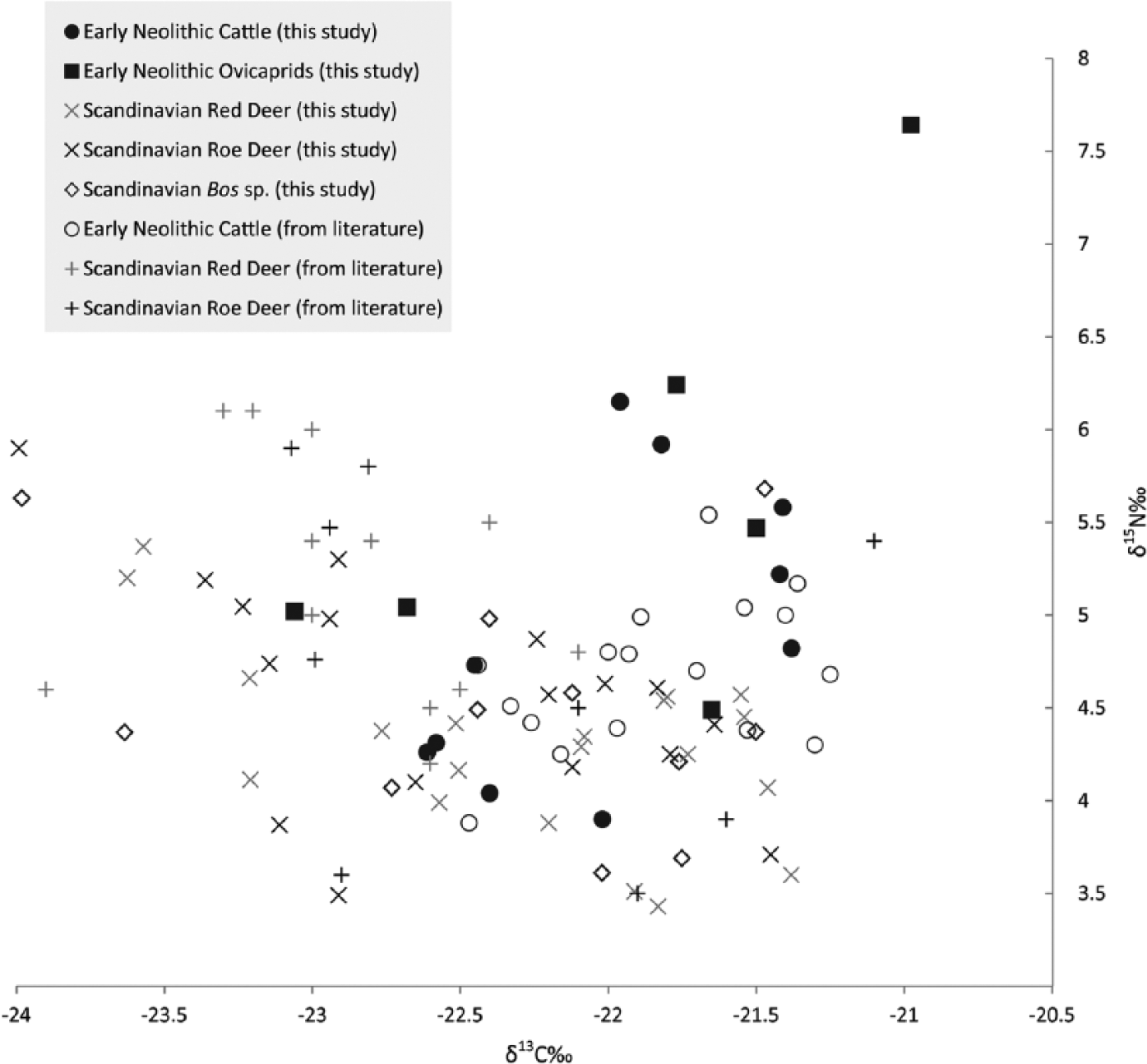
Bone collagen carbon and nitrogen isotope data from EBK and ENI fauna. Literature data from Craig et al. (2006), Fischer et al. (2007), Noe-Nygaard et al. (2005) and Ritchie et al. (2013). From literature, deer and cattle only included from EBK or ENI contexts.
In the combined new and published red deer and roe deer data, the relationship between δ13C and δ15N (Capreolus capreolus r = −0.4532, Cervus elaphus r = −0.5626) does not significantly differ between the species (Fisher r to z, z = 0.54, p = 0.5892) (Figure 3). In both cases, with increasing δ13C, δ15N decreases. Similarly, if both species of deer are divided into broad west versus east divisions by their find location on Jutland versus Zealand (Figure 1), Denmark, the relationship between δ13C and δ15N values in the deer from these geographical groupings (Jutland r = −0.461, Zealand r = −0.4568) does not significantly differ (Fisher r to z, z = −0.02, p = 0.984) (Figure 3). Therefore, neither species nor climatic differences have influenced the data. The lack of geographical differences is probably because of southern Scandinavia being too small for climate to affect values, which on a broad scale can effect a 1‰–2‰ δ13C difference on a gradient across the whole of Europe (Van Klinken et al., 1994, 2000). The lack of difference between the two species of deer is somewhat surprising, given that red deer are usually considered to primarily be grazers and roe deer are considered to primarily be browsers (Geist, 1998). This result may illustrate the extent to which the browsing behaviour of modern populations of these species of deer may be partly of anthropogenic origin. Nonetheless, because no difference can be attributed to geography or feeding preference, it must be attributed to natural differences in primary local feeding environment. In this regard, local environmental variation is known to have been high during the late Atlantic in Scandinavia (Paludan-Müller, 1978). Therefore, the observed spread of values is not surprising.
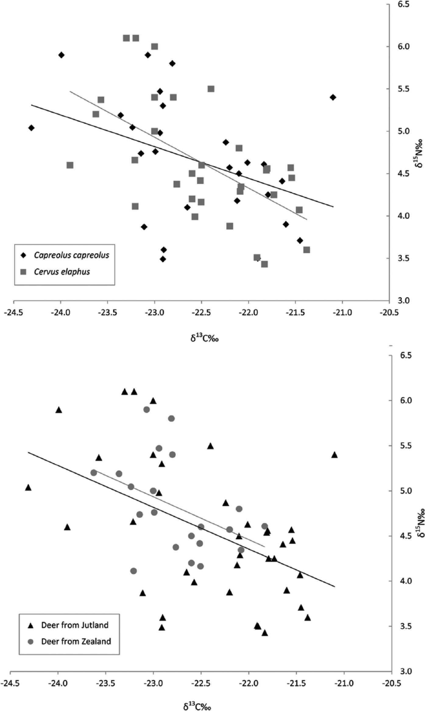
Bone collagen carbon and nitrogen isotope data. (Top) Plot of red versus roe deer. (Bottom) Plot of deer from Zealand versus Jutland. Linear regression shown.
In closed-canopy forests, δ13C values are more depleted than in open environments (van der Merwe et al., 1981). This is because closed canopies reduce air circulation and have lower light levels, both influencing factors which result in lower δ13C values (Francey and Farquhar, 1982; Noe-Nygaard, 1995). In modern populations from known environments in Denmark, higher values were seen in deer feeding in more open environments, with lower values in animals eating in more closed forests on forest floor vegetation (Noe-Nygaard, 1995). Therefore, lower values reflect feeding on plants from relatively more closed forest environments, while higher values reflect more open environments such as grasslands or open woodlands.
When pooled, both species of deer share a weak-to-moderate negative relationship between δ13C and δ15N such that as δ13C decreases, δ15N increases (r = −0.5187) (Figure 4). A similar trend was observed among late glacial and early Holocene deer from the Jura, France, where animals foraging in more closed forests had higher δ15N values owing to faster nitrogen cycling in those types of environments (Drucker et al., 2003). The relationship between degree of forest cover and nitrogen cycling, and the observed effect on these values in deer diets, is what is to be expected for herbivores feeding in the natural environment in southern Scandinavia prior to deforestation. Any population of herbivorous animals living in southern Scandinavia should therefore show a similar relationship between increasing degree of forest closure and increasing rate of nitrogen cycling.
Combining the new data from our study with the ENI values from Noe-Nygaard et al. (2005), 28 δ13C and δ15N values are available for early domestic cattle from southern Scandinavia (Figure 2). The cattle data show a relationship between δ13C and δ15N roughly opposite that of the deer. With increasing δ13C, δ15N values increase in a weak-to-moderate positive correlation (r = 0.525) (Figure 4). In comparison with the pooled deer, this difference is significant (Fisher r to z, z = 4.83, p < 0.01), as it is between cattle and the red deer (Fisher r to z, z = 4.5, p < 0.01) and cattle and roe deer (Fisher r to z, z = 3.75, p < 0.01), respectively. On these grounds, we can reject the null hypothesis that the variation in cattle diets is similar to the variation in the deer diets. The variability between cattle is not reflective of herbivore natural variation in feeding environments.
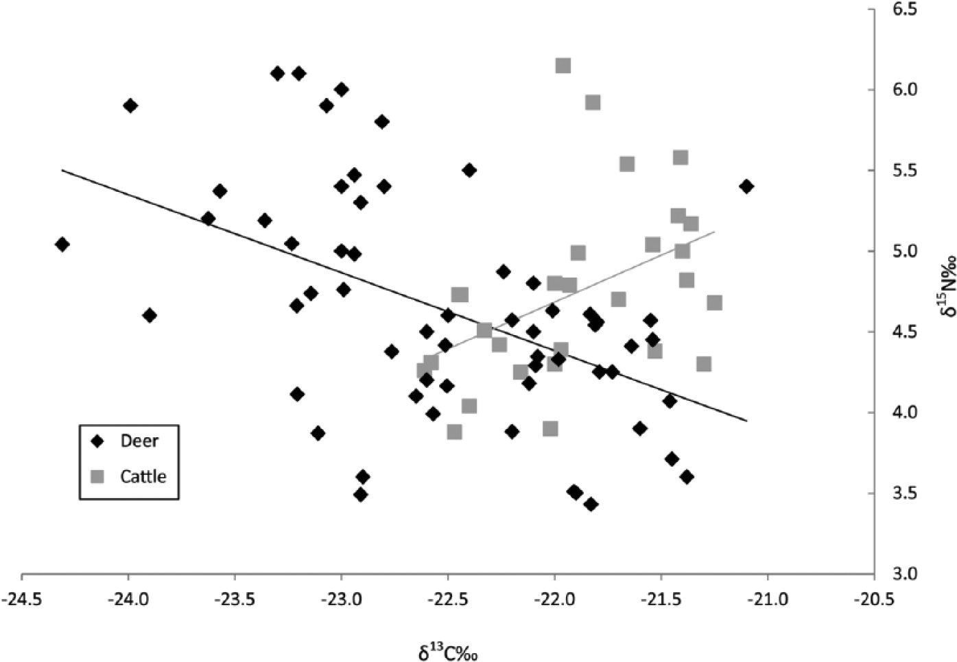
Deer versus cattle carbon and nitrogen isotope data. Linear regression shown.
Not all the cattle were, however, eating in environments wholly different to the deer. Some individual cattle had diets that approximate those of the deer, both in δ13C and in δ15N. Importantly, almost all early domestic cows from the region have δ13C values higher than −22.5‰, the general cut-off for herbivores in Europe consuming only closed-canopy plants (Drucker et al., 2003). Noe-Nygaard et al. (2005) argued that cattle were being raised in more open environments outside of those utilized by deer. However, this was based on a comparison only with the deer from two sites in the Store Åmose in central Zealand. Our broader sample of herbivores shows a significant and marked overlap between the environments where cattle were grazed (or from where cattle fodder was obtained) and the wild herbivores from the region. Average values for the cattle are higher than for the wild herbivores, but there is no clear separation between them. Perhaps this is unsurprising: our larger sample of deer from a number of sites helps to establish the normal range of expected variation in deer diets.
Drucker et al. (2003) explain the covariance between δ13C and δ15N values in deer as reflective of increased nitrogen cycling in more closed forest environments. While this appears to be the case with the Scandinavian deer sample as well, the opposite trend within the cattle requires explanation. Simply, the nitrogen values of some cattle are too high for the open environments the δ13C values indicate. Nitrogen cycling in ecosystems is a complicated process, and δ15N values in isotopic studies of diet are most often used in determination of increases in omnivorous or carnivorous species of about 3–5‰ per trophic level (Bocherens and Drucker, 2003). While not on this order of magnitude, any trophic-level effect can be soundly dismissed as deer and cattle are obligate herbivores.
Changes in aridity can contribute to δ15N values (Heaton et al., 1986). However, major changes in rainfall pattern are unlikely to have affected only the forest-dwelling deer and the open-environment cattle. Therefore, the observed pattern must be anthropogenic. However, identifying which specific human activities are causing the increase in the cattle δ15N is problematic. The two most obvious explanations are the burning of vegetation and the application of animal manure. Feeding in agricultural landscapes has been shown to increase consumer dietary δ15N values compared with conspecifics feeding in non-agricultural areas, despite the two having similar δ13C values (Hobson, 1999). Similarly, burned environments increase nitrogen cycling in plants, such that those growing in such environments have higher δ15N values and with the resulting effects on consumer values (Grogan et al., 2000). Since the repeated burning associated with slash and burn cultivation probably did not take place (see above), a more likely option is widespread manuring. This similarly causes increased δ15N values in crops (Bogaard et al., 2007, 2013). Although, in order for this increase to be subsequently seen in cattle they would either need to feed on the crops themselves, which is unlikely, or on regenerating undergrowth in fallow fields that had been manured. Regardless of the specific cause, which may be a combination of factors, the cattle are at least in part feeding in built human agricultural environments.
Discussion and conclusion
Our results amplify and extend several aspects of early Scandinavian Neolithic cattle husbandry and agriculture. Foremost, cattle dietary variation does not follow the natural pattern of environmental variation in wild herbivore diets. Second, early domestic cattle were indeed feeding in open environments such as grasslands or open woodland, as has been previously determined (Noe-Nygaard et al., 2005). These environments, however, were in part shared with wild herbivores. The data also demonstrate the presence of unambiguously human-created environments in the earliest Neolithic, the practice of animal husbandry within those areas and a particular preference for animal husbandry within a particular type of environment: open areas outside of the closed forest. These data support the notion of early Neolithic forest clearance, albeit on a small scale. These created open environments were where people carried out both cultivation and animal husbandry. This serves to contextualize cattle husbandry within the Neolithic environment of southern Scandinavia as seen in the palynological record.
The degree of deforestation largely depends on the intensity and duration of farming after initial clearance (Boserup, 1965). The practice of feeding leaves from forest trees to domestic animals only disappeared after the Second World War. In the 19th century, forest resources were a major foddering resource for domestic livestock (Slotte, 2001). Our data, however, do not indicate substantial use of forest resources for browsing in the earliest Neolithic. Deep forests were not used for cattle grazing, and forest products were not extracted for cattle fodder. Nevertheless, some of the more open environments may have included coppiced woodlands (Göransson, 1988) because in such environments much more light reaches the ground. Such an environment could result in the observed carbon values.
Most researchers agree that there appears to be a delay of about half a millennium between the appearance of domestic plants and animals in southern Scandinavia and evidence of widespread agricultural activity in the landscape (Price and Noe-Nygaard, 2009; Sørensen, 2014). Using models of agricultural origins and landscape and land-use change, this period would best be considered the Frontier Phase (cf. Mustard et al., 2004), corresponding to the Substitution Phase as defined by Zvelebil and Rowley-Conwy (1984) (Zvelebil, 1986). The speed of the transition from an undisturbed landscape to a managed or agricultural landscape depends on the individual setting, numbers of individuals involved, and a range of other factors. It can vary greatly in timescale: from decades to almost a millennium (Mustard et al., 2004). The period in southern Scandinavia from the appearance of domestic plants and animals to the appearance of evidence of large-scale agricultural activity fits well into this timeframe.
Causality is difficult to assess in the archaeological record. In particular, decisions made concerning all aspects of animal husbandry must be accessed by working backwards from the available evidence, which in this case consists of the diets of domestic species. Questions regarding the behaviour of wild species are in some ways easier to address because it is possible to observe their behavioural ecology today. However, such observations may be biased: red deer and roe deer are today considered to be predominantly grazers and browsers, respectively, yet in this dataset we see no dietary difference between them. What is clear is that the cattle were raised in more open environments outside of the closed forest, and some of these environments were created by human groups to be this way. This strongly implicates culturally normative ideas on the part of early Neolithic decision-makers about how and where to raise their cattle.
It is easy to dismiss such ideas as conjecture or simply argue that it is better to raise cattle in open environments. However, modern studies show that this is not strictly the case. For example, there are over 100 localities in Britain today in which cattle are grazed in forests (Armstrong et al., 2003). The farmers evidently had preconceived ideas of where to graze cattle and went so far as to create environments they regarded as appropriate. This speaks to entrenched cultural ideas of propriety in this regard. It is tempting to suggest that cultural preference and knowledge to perform this type of husbandry must have developed elsewhere and brought into southern Scandinavia, since indigenous hunter-gatherers adopting a few domestic cattle would not intrinsically ‘know’ that more open environments were ‘better’. We have argued elsewhere (Gron et al., 2015) that there was a degree of sophistication involved in ENI farming, which implies that the first farmers were immigrants. At all events, ENI farmers, for whatever reason, preferred open environments sufficiently strongly to create them.
It is important to remember that cattle must have played a pivotal – perhaps the pivotal – role in the earliest agriculture in the region. Perhaps their most important purpose was to buffer against crop failure and serve as a food storage mechanism (Krummel et al., 1986). As dairying was practised (Craig et al., 2011; Gron et al., 2015), cattle provided a means of obtaining fresh food through the winter, as well as a means of turning foods that are inedible to humans into meat. These data underscore not just the importance of domestic animals in the early Neolithic, but also to their role in an integrated Neolithic regime of stock keeping and small-scale agriculture for cereal production.
Footnotes
Acknowledgements
Thanks are owed to Søren H. Andersen, Elisabeth Rudebeck and T. Douglas Price for permission for the analyses and to the Zoological Museum of the Natural History Museum of Denmark, Moesgård Museum and the Malmö Museum for arranging access. We are indebted to the University of Bradford’s Stable Isotope Facility, the University of Waterloo, the CHRONO Centre at the Queen’s University Belfast and the former Department of Geology and Geography at Copenhagen University for analytical and laboratory support. We acknowledge the contributions of Inge Juul, Janet Montgomery, Nanna Noe-Nygaard, Travis Pickering, Jim Burton, Kristian Murphy Gregersen and Julia Beaumont. Harry Robson, Tina Jakob and Charlotte King greatly improved the content of earlier versions of the paper and we finally acknowledge Carolyn Freiwald who broke an analytical impasse with her thoughtful comments on the dataset.
Declaration of conflicting interests
The author(s) declared no potential conflicts of interest with respect to the research, authorship and/or publication of this article.
Funding
This research was supported by a British Academy Newton International Fellowship awarded to KG. Further funding was provided by the National Science Foundation (DDIG #1135155).