Improved control of integrating cascade processes with time delays using fractional-order internal model controller with the Smith predictor

Abstract

This article proposes an enhanced control of integrating cascade processes. The importance of the scheme shows by controlling a double integrating process with time delay under significant parametric uncertainties and load disturbances. A novel design is proposed based on the Smith predictor principle and uses a fractional-order internal model controller in the outer loop. The required fractional-order tuning parameter follows the desired gain and phase margins. At the same time, another tuning parameter, such as the fractional filter’s time constant, is calculated from the desired performance constraint. Numerical analysis and comparison are performed to showcase the feature of the hybrid structure. The simulation results show that the fractional-order internal model controller–based scheme provides enhanced tracking and faster regulation capabilities and works well under nominal and parameter uncertainty conditions.

Introduction

This article makes original contributions to two areas of controller design. They are second-order integrating plus time delay (IPTD) plants and fractional-order theory into internal model control (IMC) design. Therefore, the background concerning each of the two domains is first reviewed. The series-cascade control structure (SCCS) is a prime focus of this work.

The second-order or double integrating plant with time delay is ramping and relatively slows due to its considerable time constant. This plant primarily possesses two poles at origin, has a non-self-regulating nature, and is disturbed easily with a minor load disturbance. It is due to poor performance rejecting load disturbance by a conventional feedback system and deviating the controlled variable from a setpoint. Therefore, the controlling method requires a structural change or additional controllers to handle such plants. In this area, a cascade control structure has been adopted widely in plant industries, such as level, temperature, pressure, and flow control loops. Franks and Worley ¹ had introduced an SCCS. The closed-loop performance was improved using the inner loop by rejecting disturbances quickly. Such cascade control structure consists of two control loops. The inner-loop controller is called the secondary or slave controller, whereas the outer-loop controller is called the primary or master controller. In a typical cascade structure, faster dynamics of the inner loop help in speedier disturbance attenuation, thus minimizing the effect of disturbance before they affect the primary output. Another objective of cascade control is to minimize the sensitivity of the primary plant gain variations. However, the control strategy in cascade is more complex than a single-loop control. The structure also measures an additional output and controller to be tuned.

In industries, two different cascade controllers can be seen. The control and disturbance signals affect the primary output response through the secondary or inner loop in series-cascade control. In parallel-cascade control, the control and disturbance signals simultaneously affect primary and secondary outputs. ² Researchers in the last decade discussed the design and analysis of cascade control techniques for improved tuning and performances^3–8 and references within. It was found in the literature also a plant with input time delay or dead time could add more complexity to cascade control. The input delay increases the phase lag, leading to a decrease in gain margin and phase margin, finally leading to instability. The work with this kind of plant is a difficult task.

Our focus in this article is the cascade control method for integrating time delay plants. Therefore, the research on series-cascade control design with integrating plants is reviewed in the following. In Kaya and Atherton, ⁹ a cascade integrating time delay plant was controlled using a proportional–integral (PI)-proportional–derivative (PD) scheme with the Smith predictor (SP) in the outer loop and IMC in the inner loop. An SP-based cascade control structure was seen in Uma et al., ¹⁰ in which a secondary loop was again designed using IMC. Nevertheless, a primary loop was tuned using the direct synthesis technique for better setpoint and load disturbance rejection. A modified cascade control system was proposed in Padhan and Majhi ¹¹ using SP and IMC rules and involved two controllers and a setpoint filter. Another scheme presented in Nandong and Zang ¹² for multi-scale cascade control consisting of four controllers was applicable to self-regulating, double integrating, and unstable plants. An online tuning method in cascade control was developed by Jeng ¹³ for higher-order plants. An SP strategy was continued for cascade control to enhance the performance. In Çakıroğlu et al., ¹⁴ higher-order models were decomposed into first-order models, and depending on the order of the model, a separate loop was established. A modified cascade controller is based on the method of moments and the Routh stability criterion developed in Raja and Ali. ¹⁵ Recently, a frequency domain method with model matching was discussed for cascade controllers ¹⁶ in a nonlinear continuous stirred tank reactor.

Nowadays, fractional-order controllers (FOCs) in engineering applications are evolving into an attractive area.^17–19 The methods with FOC provide an extra degree of freedom in tuning parameters. The fractional-order proportional–integral–derivative (FOPID) presented by Podlubny ²⁰ has two additional parameters: fractional differential and fractional integral orders. Since then, many tuning approaches based on FOPID structures have been proposed in the literature. It has also seen some variations with fractional-order derivatives in the SP and IMC schemes. The fractional-order PI plus D controller was developed for integrating plants using the explicit formulae of the complex root boundary. ²¹ This method and some references within have shown better tracking performance than the classical approaches. It has been found recently a type of controller like $\mathrm{FO}{I}^{1-\lambda }{D}^{\lambda }$ using a fractional integrator and derivative actions. Oustaloup recursive approximation (ORA) method is used to implement this controller. ²² Fractional calculus was also applied in the IMC theory. Arya and Chakrabarty ¹⁸ discussed fractional-order internal model controller (FOIMC) scheme using the gain and phase margins’ specifications. Similarly, Ranjan and Mehta ²³ presented a superiority using a fractional-order tilt double derivative (FOTDD) in the IMC framework. Also, a new double-loop control approach was proposed for a time-delayed unstable system that uses a PD/P controller in its inner loop and FOIMC in its outer loop. ²⁴ To continue, Shweta et al. ²⁵ developed a novel dual-loop hybrid control method for second-order unbounded plants with dead time and zeros. In this method, an external-loop controller was designed using the FOIMC, whereas the internal-loop controller used a simple proportional–integral–derivative (PID). Kumar et al. ²⁶ suggested FOIMC for achieving satisfactory servo performance and PD to reject the disturbance rejection. It is observed the performance was improved with dual-loop and fractional-order than before. ²⁷ A compensator-based series-cascade control with FOIMC was proposed for unstable processes in Mukherjee et al. ²⁸ In Chandran et al. ⁷ and Pashaei and Bagheri, ²⁹ the secondary controller was designed from FOIMC. In general, it is noticed that the fractional-order filter in IMC can provide a more flexibility to modify the output performances. However, there are some limitations to the available methods and those are presented below.

The literature review suggested that the available methods often consume much time in computing parameters when the cascade control is used. Also, a few methods are available for integrating plants; specifically, double integrating plants are significantly less. If the integrating plant is affected by load disturbance, it will further deteriorate the relationship between input and output. Moreover, many real-time plant models contain time delays. Even considering a large time delay in plants, the perturbation may lead to poor performance. A considerable number of works have been proposed on this subject. However, they may require more tuning parameters or controllers in a loop or complex design approach. Despite some modifications suggested in the structure, the results showed poor disturbance rejection and robustness. These investigations have assisted in understanding the necessary and developing a new control scheme for cascade controlling of integrating plants. Briefly, the contributions of this article comprise as follows:

• The improved structure is suggested with only one fractional-order parameter, and a hybrid scheme contains the merits of both IMC and SP principles.

• This method can handle highly sensitive processes under parametric uncertainties and load disturbances.

• The fractional-order parameter in the controller could be selected based on gain margin $(g_m)$ and phase margin $({\varphi }_m)$ specifications. The desirable range is provided for ease of selection tasks. The fractional-order IMC filter’s time constant is tuned by the balanced, objective function under constraints.

• The robustness study is performed to demonstrate the advantages of the proposed scheme, which includes parameter perturbation, external and internal load disturbances, and noisy output signal.

• The quantitative analysis also shows superior performances compared with recently developed works.

The article is organized as follows. Section “Preliminary” represents the general IMC scheme and tilt–integral–derivative (TID) controller. In sections “Plant models, controller, and tuning procedures” and “The proposed controller design in real-time,” the proposed controlling scheme is discussed in detail. Then, the selection of tuning parameters is suggested in section “Tuning of $\lambda$ and $\beta$ for the proposed controller structure.” Section “Robustness analysis and stability” presents the robustness and stability analysis of the proposed controller. The numerical simulation is performed in section “Simulation results,” compared with other methods, and finally, the conclusion is given in section “Conclusion.”

Preliminary

This section presents the basic IMC structure and equations related to it and also some details about the series-cascade control system.

The general IMC control system

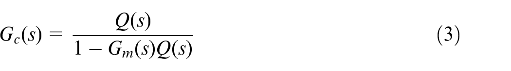
The well-known IMC scheme is shown in Figure 1, where $G_p(s)$ , $G_m(s)$ , $Q(s)$ , and $G_c(s)$ representing the plant, plant model, IMC controller, and feedback controller, respectively. The design procedure using the IMC principle can be seen briefly below.

• Step 1: factorize the plant model, $G_m$ into two parts. $G_m^{-}$ as invertible and minimum phase. $G_m^{+}$ as non-invertible and non-minimum phase parts (delays and right half-plane zeros)

$$G_m(s)=G_m^{+}(s)G_m^{-}(s)$$

(1)

• Step 2: take inversion for invertible part $G_m^{-}$ .

• Step 3: add a low-pass filter $f(s)$ in order to make IMC controller proper. Then, the IMC controller becomes

$$Q(s)=G_m^{-}(s{)}^{-1}f(s)$$

(2)

• Step 4: the simplified form of the feedback controller is obtained as

$$G_c(s)=\frac{Q(s)}{1-G_m(s)Q(s)}$$

(3)

Figure 1.

Typical IMC structure.

The fractional-order tilt–integral–derivative controller

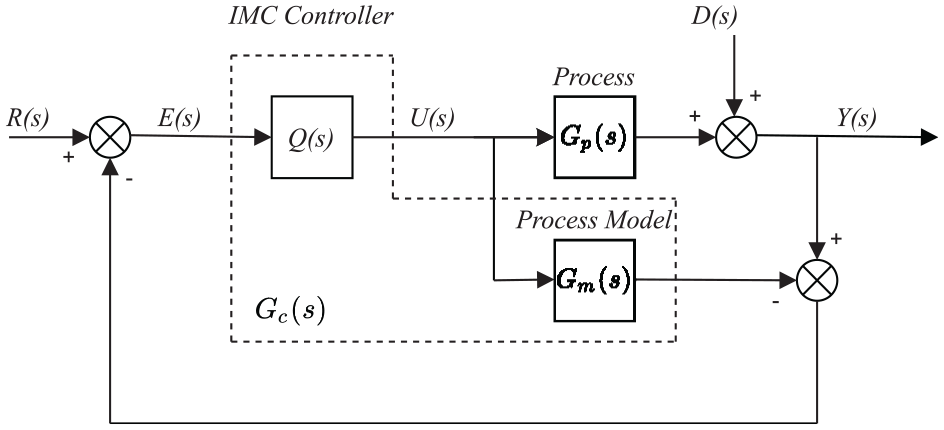
The well-known FOPID involves the tuning of five parameters: commonly gains $K_p$ , $K_i$ , $K_d$ and fractional orders $\alpha$ and $\mu$ . It has been demonstrated in the literature that it can offer additional flexibility to meet design control goals. The TID controller also belongs to the same fractional-order family. Despite having only four parameters, the structure is almost identical to the widely used PID. Only the proportional gain is replaced by the tilted gain $(K_t)$ having a transfer function $1/s^{\frac{1}{n}}$ , where $n$ is a non-zero real number. ³⁰ The standard transfer function of TID controller can be represented as

$$\mathrm{TID}=K_t\frac{1}{s^{\frac{1}{n}}}+K_i\frac{1}{s}+K_{d}s$$

(4)

where $K_t$ is the tilted gain, $K_i$ is the integral gain, and $K_d$ is the derivative gain. The tuning parameter, $n$ should be between the numbers 2 and 3. A TID controller exhibits more accurate tuning, quick disturbance rejection, and minimizes parameter uncertainty when compared to conventional controllers. The study of this topic has recently attracted a lot of interest. A robust 3-degree-of-freedom (3DOF)-TID controller ³¹ as well as integral derivative-tilted (ID-T) controller ³² developed for load frequency control in interconnected power systems was some of the works developed recently. The transfer function of the controller can be written below

$$\mathrm{FOTID}=K_t\frac{1}{s^{\frac{1}{n}}}+K_i\frac{1}{s^{\alpha }}+K_d{s}^{\mu }$$

(5)

where $\alpha$ and $\mu$ are the positive real orders for integral and derivative, respectively. Here, we want to apply the IMC principle designing the fractional-order tilt–integral–derivative (FOTID) of form in equation (5). Aiming to make a simple tuning approach, even though the controller seems to be complex with three fractional orders. The proposed design is discussed in the following sections for integrating plant models. We attempt to obtain one common tuning parameter to calculate other parameters and use the plant information.

Series-cascade control system

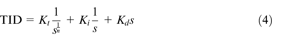
Figure 2 shows the typical structure of a series-cascade control system, which consists of two control loops, namely, the inner loop with plant $G_{p2}$ and the outer loop with plant $G_{p1}$ . Let us assume the load disturbances entering inner and outer loops with values $D_1$ , $D_2$ , and $D_3$ as seen in Figure 2. The primary plant-controlled variable $Y_1(s)$ with setpoint $R_1(s)$ is used by the primary controller $G_{c1}$ to build a setpoint for the secondary controller $G_{c2}$ . The general guideline behind this configuration is that the inner loop should be faster than the outer loop, that is, the disturbance affecting the inner loop is compensated before it affects the primary plant. The outer loop can be designed for setpoint tracking, but the problem arises when the outer plant will have a large time delay. In such cases, the SP can be used for compensating the delay.

Figure 2.

Series-cascade control structure.

Plant models, controller, and tuning procedures

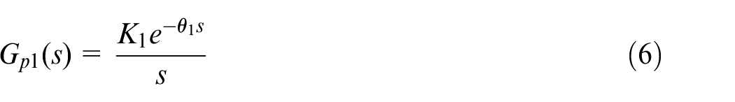
The series plant is mainly combined with the stable inner plant, whereas the primary plant may be stable, unstable, or integrating by nature. In our work, we have considered the following plant models to study. Let the IPTD model as

$$G_{p1}(s)=\frac{K_1{e}^{-{\theta }_{1}s}}{s}$$

(6)

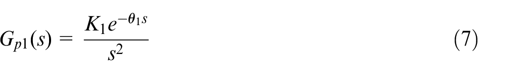
The double integrating plus time delay (DIPTD) model is

$$G_{p1}(s)=\frac{K_1{e}^{-{\theta }_{1}s}}{s^2}$$

(7)

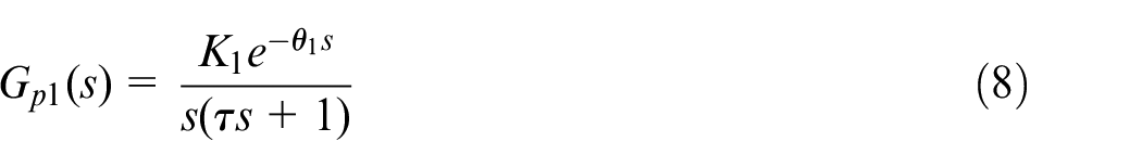
The integrating second-order plus time delay (ISOPTD) model is

$$G_{p1}(s)=\frac{K_1{e}^{-{\theta }_{1}s}}{s(\tau s+1)}$$

(8)

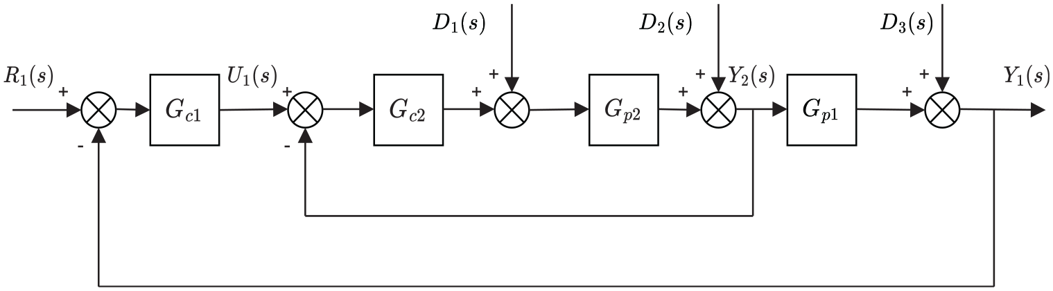
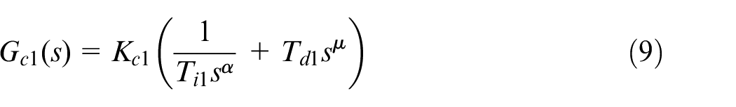
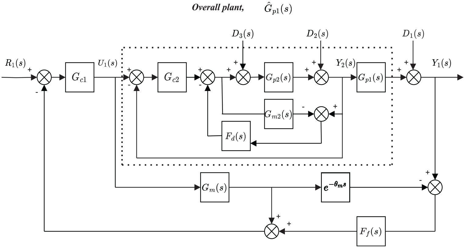
The proposed SCCS scheme is given in the block diagram (Figure 3). As seen in the figure, it has two main controllers and a filter compensator. First, the inner-loop controller is designed using the IMC principle. Following the inner loop, the outer primary controller is developed as an FOC. Aiming to design a new fractional controller for integrating plants to make the overall system more stable and robust with load disturbance inputs. Let us express the primary and secondary controllers as

$$G_{c1}(s)=K_{c1}(\frac{1}{T_{i1}{s}^{\alpha }}+T_{d1}{s}^{\mu })$$

(9)

$$G_{c2}(s)=K_{c2}(1+\frac{1}{T_{i2}s})$$

(10)

Figure 3.

Proposed series-cascade control structure for integrating plants.

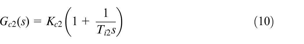
The $G_{c1}$ in equation (9) is called a fractional-order integrator and derivative (FOID) controller and $\alpha ,\mu$ are the fractional orders of the integral and differential. Also, one can use the gains $K_{c1}/\mathrm{Ti}1=K_{i1}$ and $K_{c1}{T}_{d1}=K_{d1}$ for simplifying design steps. The $G_{c2}$ in equation (10) is the classical PI controller.

The inner-loop controller design

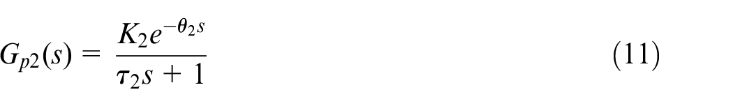
The model of a secondary process $G_{m2}(s)$ having a small time delay can be controlled effectively using the well-known simple internal model control (SIMC) tuning. ³³ Let us consider the stable first-order plus time delay (FOPTD) model as

$$G_{p2}(s)=\frac{K_2{e}^{-{\theta }_{2}s}}{{\tau }_{2}s+1}$$

(11)

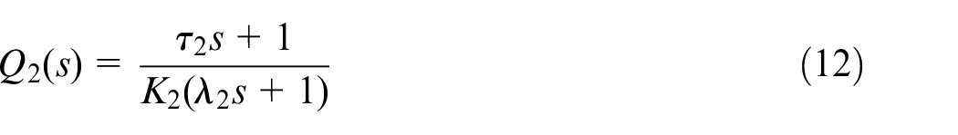
Then, following the IMC technique from section “The general IMC control system,” one can obtain the IMC controller for the inner loop as

$$Q_2(s)=\frac{{\tau }_{2}s+1}{K_2({\lambda }_{2}s+1)}$$

(12)

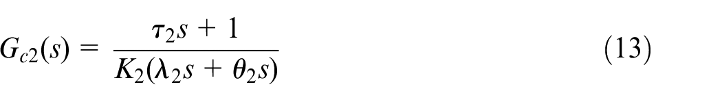
where ${\lambda }_2$ is a single tuning parameter and defined also as a secondary closed-loop time constant. From equation (3), the secondary controller can be obtained as below after approximating $e^{-{\theta }_{2}s}$ to $(1-{\theta }_{2}s)$ using the Taylor series expansion

$$G_{c2}(s)=\frac{{\tau }_{2}s+1}{K_2({\lambda }_{2}s+{\theta }_{2}s)}$$

(13)

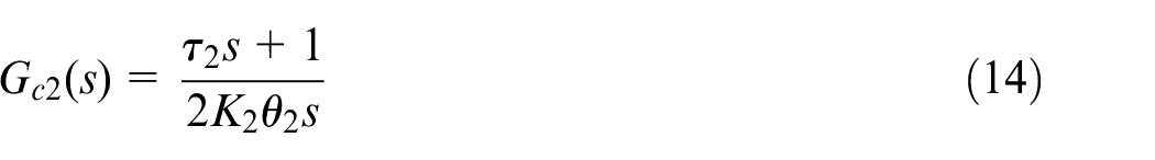
The objective of the inner controller is to reject the load disturbance before affecting the outer plant response. According to the SIMC tuning rule, a fast response with good robustness is obtained when ${\lambda }_2={\theta }_2$ . It gives further

$$G_{c2}(s)=\frac{{\tau }_{2}s+1}{2K_2{\theta }_{2}s}$$

(14)

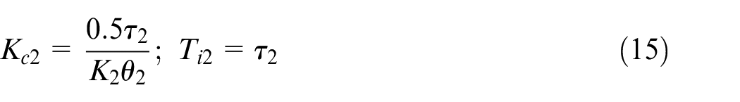
Comparing with the classical PI in equation (10), we obtain the parameter values as below

$$K_{c2}=\frac{0.5{\tau }_2}{K_2{\theta }_2};T_{i2}={\tau }_2$$

(15)

Now, the inner-loop transfer function is given by

$$\frac{Y_2(s)}{U_1(s)}=\frac{G_{c2}(s)G_{p2}(s)}{1+G_{c2}(s)G_{p2}(s)}$$

(16)

Substitution $G_{p2}$ and $G_{c2}$ in equation (16) gives

$$\frac{Y_2(s)}{U_1(s)}=\frac{0.5e^{-{\theta }_{2}s}}{{\theta }_{2}s+0.5e^{-{\theta }_{2}s}}$$

(17)

After replacing the small value time delay $e^{-{\theta }_{2}s}=1-{\theta }_{2}s$ , the approximated inner-loop becomes

$$\frac{Y_2(s)}{U_1(s)}\approx \frac{e^{-{\theta }_{2}s}}{{\theta }_{2}s+1}$$

(18)

Since it is straightforward to simplify the inner-loop, the primary controller can be designed from the following section.

The proposed outer-loop controller design

To design the main loop controller, the overall plant transfer function can be considered after the modified inner loop as below

$$\begin{array}{c}\multicolumn{1}{c}{{\hat{G}}_{p1}=G_{p1}{e}^{-{\theta }_{1}s}\frac{Y_2(s)}{U_1(s)}=\frac{G_{p1}{e}^{-{\theta }_{1}s}{e}^{-{\theta }_{2}s}}{{\theta }_{2}s+1}\approx G_{p1}{e}^{-({\theta }_1+2{\theta }_2)s}}\\ \multicolumn{1}{c}{=G_{p1}{e}^{-{\theta }_{m}s}}\end{array}$$

(19)

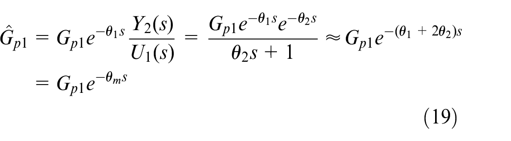
where ${\theta }_m$ represents the overall time delay, and ${\hat{G}}_{p1}$ represents the total plant transfer function.

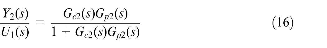
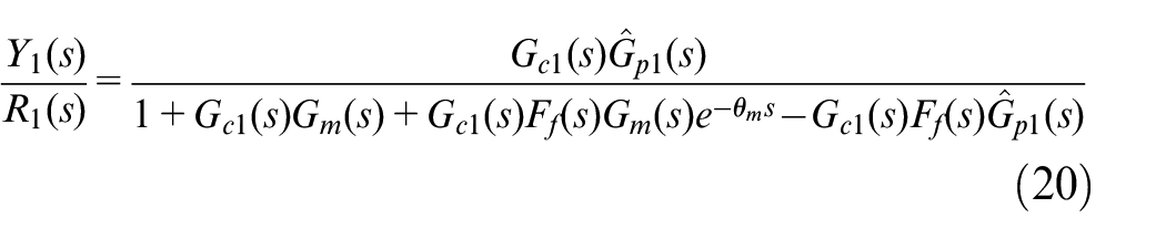
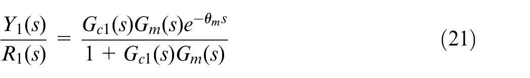
The overall primary closed-loop transfer function for servo response can be written as

$$\begin{array}{c}\multicolumn{1}{c}{\frac{Y_1(s)}{R_1(s)}=\frac{G_{c1}(s){\hat{G}}_{p1}(s)}{1+G_{c1}(s)G_m(s)+G_{c1}(s)F_f(s)G_m(s)e^{-{\theta }_{m}s}-G_{c1}(s)F_f(s){\hat{G}}_{p1}(s)}}\end{array}$$

(20)

By considering the model exactly represents the process $({\hat{G}}_{p1}(s)=G_m{e}^{-{\theta }_{m}s})$ , equation (20) can be represented as

$$\frac{Y_1(s)}{R_1(s)}=\frac{G_{c1}(s)G_m(s)e^{-{\theta }_{m}s}}{1+G_{c1}(s)G_m(s)}$$

(21)

Case 1: IPTD plant

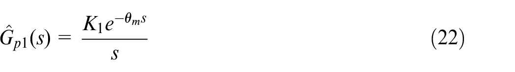
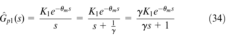
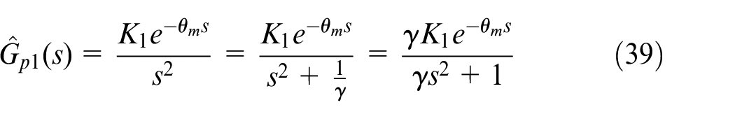
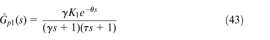
Let us take $G_{p1}$ as equation (6), where $K_1$ is the static gain and ${\theta }_1$ is a dead time. Using equation (19), the overall transfer function for the outer loop becomes

$${\hat{G}}_{p1}(s)=\frac{K_1{e}^{-{\theta }_{m}s}}{s}$$

(22)

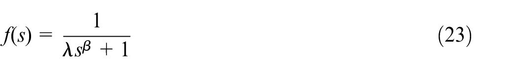
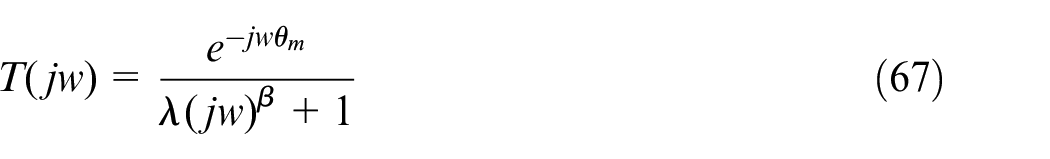
where ${\theta }_m=2{\theta }_2+{\theta }_1$ . Aiming to design a fractional-order IMC filter, we have chosen the form of IMC filter with fractional-order differentiator as below

$$f(s)=\frac{1}{\lambda s^{\beta }+1}$$

(23)

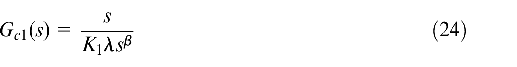
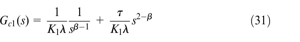
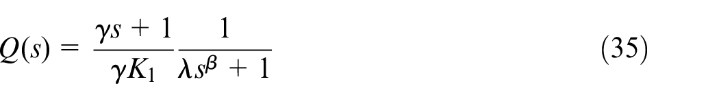
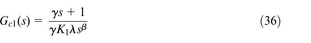
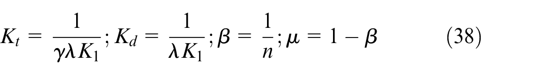
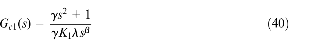
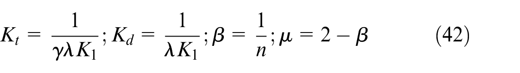
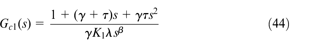
where $\lambda$ represents a fractional filter time constant ( $\lambda >0$ ) and $\beta$ is a positive real number, that is, the fractional order $\beta$ , lies in the range $0\le \beta \le 2$ . The value of $\beta$ varies with different plants, and the choice of $\beta$ as per plant type is further discussed in section “Choice of β.” Now, according to the IMC rule, one can obtain the outer-loop controller $G_{c1}$ using equation (3). Following the basic rule of the IMC, the FOC becomes

$$G_{c1}(s)=\frac{s}{K_1\lambda s^{\beta }}$$

(24)

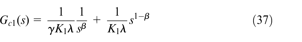
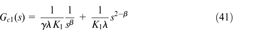
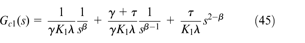
The above equation can be seen as a fractional-order D controller as below

$$G_{c1}(s)=\frac{1}{K_1\lambda }{s}^{1-\beta }$$

(25)

$$G_{c1}(s)=K_{d1}{s}^{1-\beta }$$

(26)

where $K_{d1}=1/K_1\lambda$ . The overall closed-loop transfer function after substituting in equation (21) can be obtained as

$$\frac{Y_1(s)}{R_1(s)}=\frac{e^{-{\theta }_{m}s}}{\lambda s^{\beta }+1}$$

(27)

Case 2: DIPTD plant

The DIPTD plant in equation (7) can obtain the outer controller as below after the inner-loop transformation

$$G_{c1}(s)=\frac{s^2}{K_1\lambda s^{\beta }}$$

(28)

Finally, the outer controller is obtained as below

$$G_{c1}(s)=K_{d1}{s}^{2-\beta }$$

(29)

Case 3: ISOPTD

The ISOPTD plant in equation (8) is formed as the outer controller as below

$$G_{c1}(s)=\frac{s(\tau s+1)}{K_1\lambda s^{\beta }}$$

(30)

The above equation can be rearranged as below

$$G_{c1}(s)=\frac{1}{K_1\lambda }\frac{1}{s^{\beta -1}}+\frac{\tau }{K_1\lambda }{s}^{2-\beta }$$

(31)

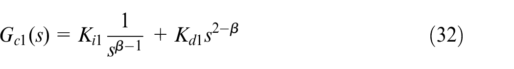
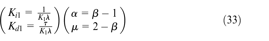
This can be denoted as an FOID controller

$$G_{c1}(s)=K_{i1}\frac{1}{s^{\beta -1}}+K_{d1}{s}^{2-\beta }$$

(32)

and its parameters become

$$\left(\begin{array}{c}{K}_{i1}=\frac{1}{K_1\lambda }\hfill \\ \multicolumn{1}{c}{K_{d1}=\frac{\tau }{K_1\lambda }}\end{array}\right)\left(\begin{array}{c}\alpha =\beta -1\hfill \\ \multicolumn{1}{c}{\mu =2-\beta }\end{array}\right)$$

(33)

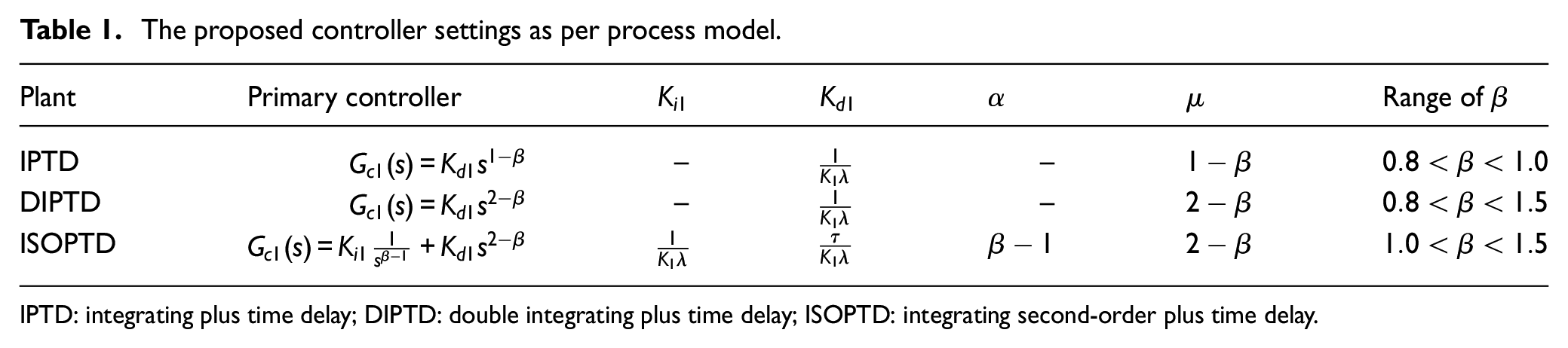
As per the transfer function models of the outer process, the controller settings are tabulated in Table 1.

Table 1.

The proposed controller settings as per process model.

Plant	Primary controller	$K_{i1}$	$K_{d1}$	$\alpha$	$\mu$	Range of $\beta$
IPTD	$G_{c1}(s)=K_{d1}{s}^{1-\beta }$	–	$\frac{1}{K_1\lambda }$	–	$1-\beta$	$0.8<\beta <1.0$
DIPTD	$G_{c1}(s)=K_{d1}{s}^{2-\beta }$	–	$\frac{1}{K_1\lambda }$	–	$2-\beta$	$0.8<\beta <1.5$
ISOPTD	$G_{c1}(s)=K_{i1}\frac{1}{s^{\beta -1}}+K_{d1}{s}^{2-\beta }$	$\frac{1}{K_1\lambda }$	$\frac{\tau }{K_1\lambda }$	$\beta -1$	$2-\beta$	$1.0<\beta <1.5$

IPTD: integrating plus time delay; DIPTD: double integrating plus time delay; ISOPTD: integrating second-order plus time delay.

The proposed controller design in real-time

Let us take first ${\hat{G}}_{p1}(s)$ from equation (22), where $K_1$ is the static gain and ${\theta }_m$ is a dead time. This IPTD model can be approximated into the FOPTD model as below

$${\hat{G}}_{p1}(s)=\frac{K_1{e}^{-{\theta }_{m}s}}{s}=\frac{K_1{e}^{-{\theta }_{m}s}}{s+\frac{1}{\gamma }}=\frac{\gamma K_1{e}^{-{\theta }_{m}s}}{\gamma s+1}$$

(34)

where $\gamma$ is considered as a constant with a high value, say $\gamma =100$ . As per the new filter equation (23), the resulting IMC controller becomes

$$Q(s)=\frac{\gamma s+1}{\gamma K_1}\frac{1}{\lambda s^{\beta }+1}$$

(35)

It can be realized as the feedback controller from equation (3) below

$$G_{c1}(s)=\frac{\gamma s+1}{\gamma K_1\lambda s^{\beta }}$$

(36)

The above equation can be rearranged with respect to TD controller in equation (5). In this case, one can see the expression as

$$G_{c1}(s)=\frac{1}{\gamma K_1\lambda }\frac{1}{s^{\beta }}+\frac{1}{K_1\lambda }{s}^{1-\beta }$$

(37)

Comparing equations (37) and (5), the TD controller values are obtained as below

$$K_t=\frac{1}{\gamma \lambda K_1};K_d=\frac{1}{\lambda K_1};\beta =\frac{1}{n};\mu =1-\beta$$

(38)

The DIPTD plant in equation (7) in the same way can be approximated as

$${\hat{G}}_{p1}(s)=\frac{K_1{e}^{-{\theta }_{m}s}}{s^2}=\frac{K_1{e}^{-{\theta }_{m}s}}{s^2+\frac{1}{\gamma }}=\frac{\gamma K_1{e}^{-{\theta }_{m}s}}{\gamma s^2+1}$$

(39)

In the same way, one can obtain the feedback controller as shown below

$$G_{c1}(s)=\frac{\gamma s^2+1}{\gamma K_1\lambda s^{\beta }}$$

(40)

The above equation can be arranged with respect to TD controller as

$$G_{c1}(s)=\frac{1}{\gamma \lambda K_1}\frac{1}{s^{\beta }}+\frac{1}{K_1\lambda }{s}^{2-\beta }$$

(41)

Comparing equations (41) and (5), the TD controller values are obtained as below

$$K_t=\frac{1}{\gamma \lambda K_1};K_d=\frac{1}{\lambda K_1};\beta =\frac{1}{n};\mu =2-\beta$$

(42)

It can be seen for IPTD and DIPTD process models that the integral part is not required. Thus, the parameter $K_i=0$ .

The ISOPTD plant in equation (8) can be represented as

$${\hat{G}}_{p1}(s)=\frac{\gamma K_1{e}^{-\theta s}}{(\gamma s+1)(\tau s+1)}$$

(43)

The feedback controller can be obtained as

$$G_{c1}(s)=\frac{1+(\gamma +\tau )s+\gamma \tau s^2}{\gamma K_1\lambda s^{\beta }}$$

(44)

The above equation can be arranged with respect to TID controller as

$$G_{c1}(s)=\frac{1}{\gamma K_1\lambda }\frac{1}{s^{\beta }}+\frac{\gamma +\tau }{\gamma K_1\lambda }\frac{1}{s^{\beta -1}}+\frac{\tau }{K_1\lambda }{s}^{2-\beta }$$

(45)

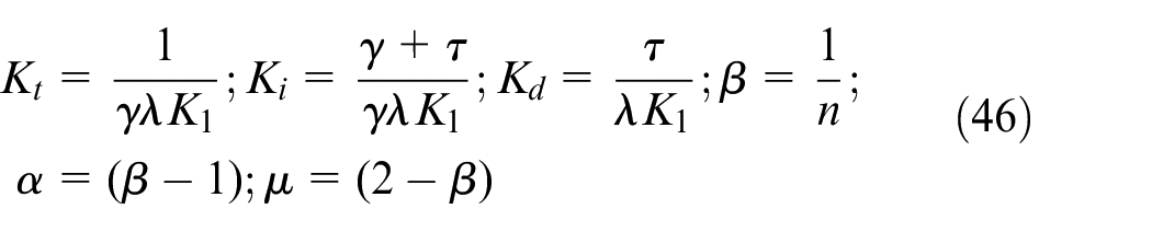
Comparing equations (45) and (5), the FOTID parameters become

$$\begin{array}{c}\multicolumn{1}{c}{K_t=\frac{1}{\gamma \lambda K_1};K_i=\frac{\gamma +\tau }{\gamma \lambda K_1};K_d=\frac{\tau }{\lambda K_1};\beta =\frac{1}{n};}\\ \multicolumn{1}{c}{\alpha =(\beta -1);\mu =(2-\beta )}\end{array}$$

(46)

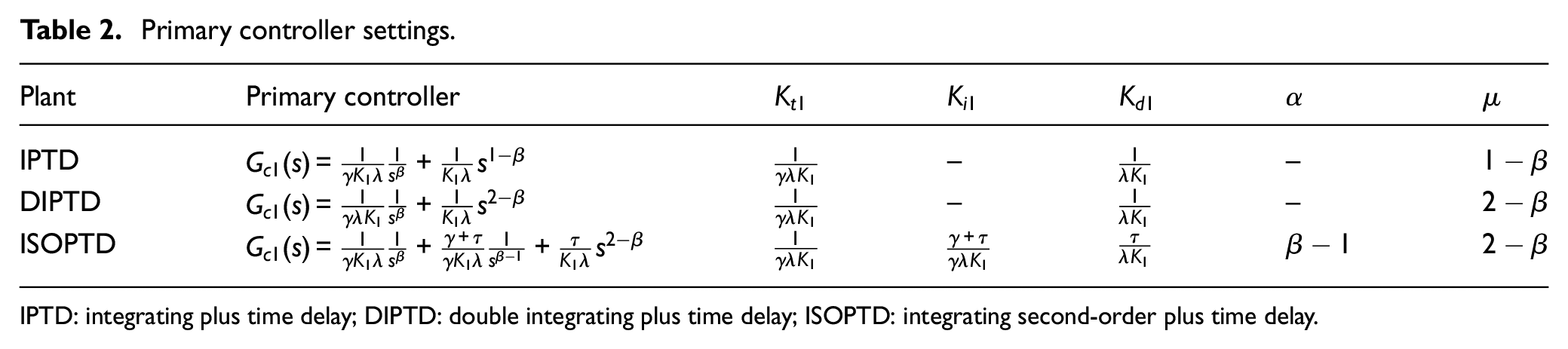
The proposed controller settings as per practical cases can be noted as shown in Table 2.

Table 2.

Primary controller settings.

Plant	Primary controller	$K_{t1}$	$K_{i1}$	$K_{d1}$	$\alpha$	$\mu$
IPTD	$G_{c1}(s)=\frac{1}{\gamma K_1\lambda }\frac{1}{s^{\beta }}+\frac{1}{K_1\lambda }{s}^{1-\beta }$	$\frac{1}{\gamma \lambda K_1}$	–	$\frac{1}{\lambda K_1}$	–	$1-\beta$
DIPTD	$G_{c1}(s)=\frac{1}{\gamma \lambda K_1}\frac{1}{s^{\beta }}+\frac{1}{K_1\lambda }{s}^{2-\beta }$	$\frac{1}{\gamma \lambda K_1}$	–	$\frac{1}{\lambda K_1}$	–	$2-\beta$
ISOPTD	$G_{c1}(s)=\frac{1}{\gamma K_1\lambda }\frac{1}{s^{\beta }}+\frac{\gamma +\tau }{\gamma K_1\lambda }\frac{1}{s^{\beta -1}}+\frac{\tau }{K_1\lambda }{s}^{2-\beta }$	$\frac{1}{\gamma \lambda K_1}$	$\frac{\gamma +\tau }{\gamma \lambda K_1}$	$\frac{\tau }{\lambda K_1}$	$\beta -1$	$2-\beta$

IPTD: integrating plus time delay; DIPTD: double integrating plus time delay; ISOPTD: integrating second-order plus time delay.

The disturbance filter for an inner loop

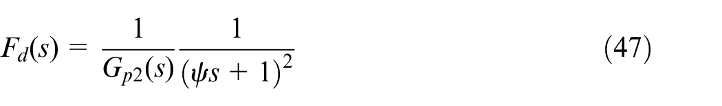
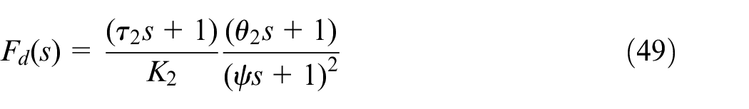
The literature suggested some restrictions with IMC and SIMC methods. They perform poorly with disturbance inputs and have less flexibility to improve performance for robustness.^3,15 It is essential to improve load rejections, especially the plants are in cascade. In our work, a disturbance filter is required in the inner loop. The tuning of a filter should be simple and based on model parameters. For that purpose, we have included a disturbance filter from the inverse model and converted it into a proper second-order filter. A general form $1/(\psi s+1{)}^2$ can be included as below into the filter, $F_d(s)$ as

$$F_d(s)=\frac{1}{G_{p2}(s)}\frac{1}{{(\psi s+1)}^2}$$

(47)

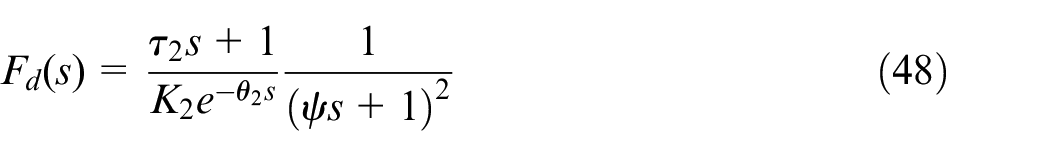
Since the inner plant model is a first-order stable, the above equation becomes

$$F_d(s)=\frac{{\tau }_{2}s+1}{K_2{e}^{-{\theta }_{2}s}}\frac{1}{{(\psi s+1)}^2}$$

(48)

The time delay can be approximated with a first-order Taylor series expansion, and then $F_d$ is expressed by

$$F_d(s)=\frac{({\tau }_{2}s+1)}{K_2}\frac{({\theta }_{2}s+1)}{{(\psi s+1)}^2}$$

(49)

A smaller value of $\psi$ results in a faster recovery, which is recommended for the cascade plants. Considering the ease of design step, $\psi$ is chosen as ${\theta }_2/2$ in this work.

The robustness filter for an outer loop

The model uncertainties are critical for any controller scheme. As seen in Figure 3, the filter, namely, $F_f$ , is included to act on errors between the actual and predicted outputs. It is also proven that a filter helps to deal with a time delay issue. ³⁴ Let us take $F_f(s)=1/{\tau }_{f}s+1$ . It is noted that a small value of ${\tau }_f$ constant yields a fast regulatory response and small settling time. Whereas a high value can result in more settling time and sluggish response. For our plant type, it is aimed to focus on robustness. After a numerical study on all integrating plant types, ${\tau }_f$ is directly related to plant time delay, and it can be taken simply as $2{\theta }_m$ .

Tuning of $\lambda$ and $\beta$ for the proposed controller structure

A plant industry is well practiced with a classical controller design from the maximum sensitivity and margins specifications. ³⁵ These specifications can handle various dynamics including small and large time delay plants. The basic concept is to convert an open-loop transfer function by choosing controller’s zeros equal to poles of the model. In the proposed work, we have considered a fractional-order pole with order $\beta$ and the loop equation becomes

$${\hat{G}}_{p1}(s)G_{c1}(s)=K{e}^{-{\theta }_{m}s}/s^{\beta }$$

(50)

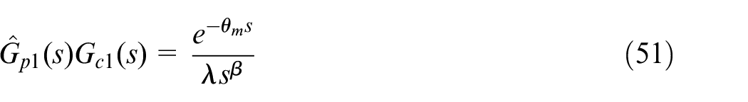
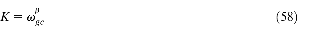
where K represents loop transfer function gain and can be determined based on gain and phase margin specifications. Now, as per plant models and their controller structures in section “The proposed outer-loop controller design,” the open-loop transfer function can be written as

$${\hat{G}}_{p1}(s)G_{c1}(s)=\frac{e^{-{\theta }_{m}s}}{\lambda s^{\beta }}$$

(51)

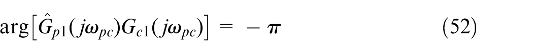
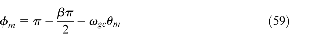
Comparing equations (50) and (51), one can easily calculate, $\lambda =1/K$ . It is to remind that a parameter $\lambda$ appears from the fractional-order filter equation (23). Now, the basic definitions for the gain and phase margins can be written as below

$$\arg [{\hat{G}}_{p1}(j{\omega }_{\mathrm{pc}})G_{c1}(j{\omega }_{\mathrm{pc}})]=-\pi$$

(52)

$$g_m|{\hat{G}}_{p1}(j{\omega }_{\mathrm{pc}})G_{c1}(j{\omega }_{\mathrm{pc}})|=1$$

(53)

$$|{\hat{G}}_{p1}(j{\omega }_{\mathrm{gc}})G_{c1}(j{\omega }_{\mathrm{gc}})|=1$$

(54)

$${\varphi }_m=\pi +\arg [{\hat{G}}_{p1}(j{\omega }_{\mathrm{gc}})G_{c1}(j{\omega }_{\mathrm{gc}})]$$

(55)

where the gain margin and phase margin as $g_m$ and ${\varphi }_m$ and their crossover frequencies as ${\omega }_{\mathrm{gc}}$ and ${\omega }_{\mathrm{pc}}$ , respectively.

Substituting equation (51) into equations (52)–(55), following set of expressions is obtained

$${\omega }_{\mathrm{pc}}{\theta }_m=\pi -\frac{\beta \pi }{2}$$

(56)

$$g_m=\frac{{\omega }_{\mathrm{pc}}^{\beta }}{K}$$

(57)

$$K={\omega }_{\mathrm{gc}}^{\beta }$$

(58)

$${\varphi }_m=\pi -\frac{\beta \pi }{2}-{\omega }_{\mathrm{gc}}{\theta }_m$$

(59)

Using equations (57) and (58), one can write

$$g_m{\omega }_{\mathrm{gc}}^{\beta }={\omega }_{\mathrm{pc}}^{\beta }$$

(60)

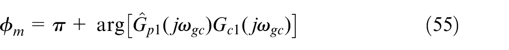
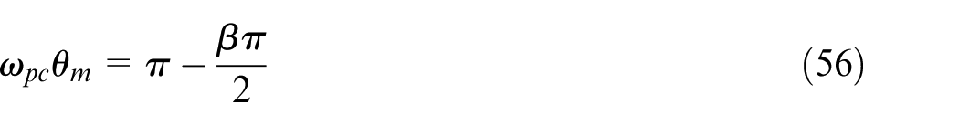
After multiplying ${\theta }_m$ both sides of equation (60) and then further modification with equations (56) and (59), the new phase and gain margin relation can be obtained as below

$${\varphi }_m=\pi -\frac{\beta \pi }{2}(1-\frac{1}{\sqrt[\beta ]{g_m}})$$

(61)

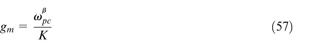
Differently from a classical relation, the above expression provides an extra parameter to tune for desired $g_m$ and ${\varphi }_m$ . This is well related to the new fractional-order ID controller. Same way, equations (56) and (57) can be modified for $\lambda$ as below

$$\lambda =\frac{g_m}{{\left(\frac{\pi -\frac{\beta \pi }{2}}{{\theta }_m}\right)}^{\beta }}$$

(62)

Now the possible values of $\beta$ are observed using relation in equation (61). As recommended values for $g_m$ are between 2 and 5 and for ${\varphi }_m$ are between $30°$ and $60°$ . The interesting result can be seen in Figure 4.

Figure 4.

Region of $\beta$ as per $g_m$ and ${\varphi }_m$ specifications.

Choice of $\beta$

According to numerical values, the typical choice of $\beta$ shall be between $0.8$ and $1.5$ . So, the fractional-order IMC filter’s parameters are bounded by recommended ranges for the gain and phase margins. As per this requirement and model type, we have found for IPTD plant selection from $0.8<\beta <1.0$ , for DIPTD plant $0.8<\beta <1.5$ and for ISOPTD plant $1.0<\beta <1.5$ . This enables the estimation task to be faster and overcomes the problem of selection gain and phase margins.

Final tuning based on a performance index

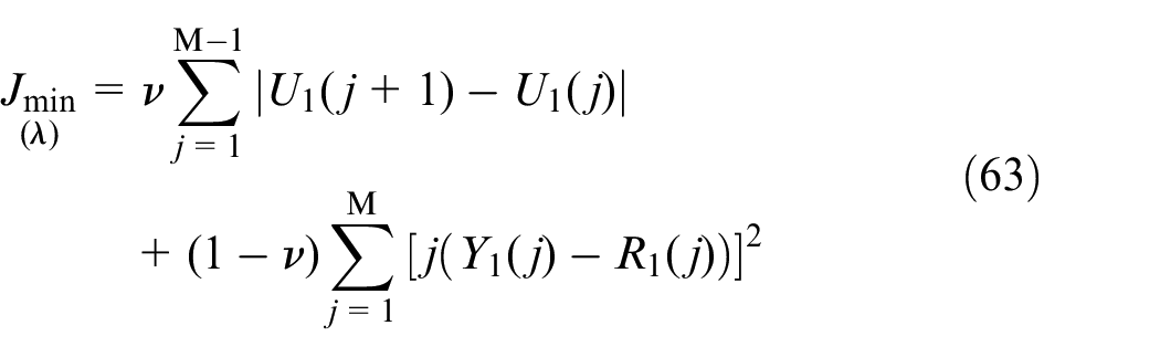
The performance criterion is defined by the following cost function equation (63) to fulfill dual requirements for given $\beta$

$$\begin{array}{c}\multicolumn{1}{c}{\underset{(\lambda )}{J_{min}}=\nu \sum _{j=1}^{\mathrm{M}-1}|U_1(j+1)-U_1(j)|}\\ \multicolumn{1}{c}{+(1-\nu )\sum _{j=1}^{\mathrm{M}}{\left[j(Y_1(j)-R_1(j))\right]}^2}\end{array}$$

(63)

where the first term calculates the control signal variations and the second term is the integral of the time-squared error. Also, $U_j$ and $Y_1(j)$ are the outer plant input and output at time $t=t_j$ , with $\mathrm{M}$ data points.

It can be seen from equation (63) that the index can tradeoffs between control signal variations and transient setpoint errors by choosing any suitable value of $\nu \in (0,1)$ . In order to guarantee robustness in the cascade control system, the parameters are calculated from the minimum of the cost function.

Summary of tuning procedure

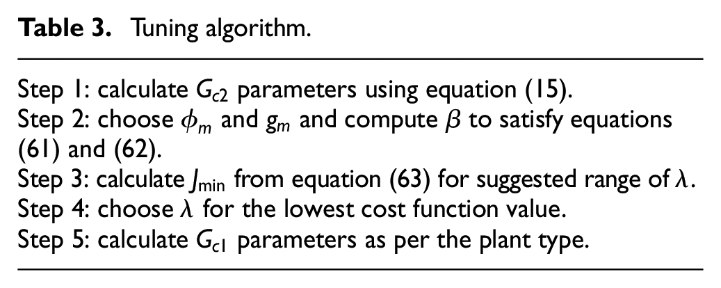
The two non-linear expressions from equations (61) and (62) are important relation in this study. The robustness and stability of any closed-loop control system are related with $g_m$ and ${\varphi }_m$ values. The proposed method’s required parameters are initially chosen from the first choice of $g_m$ and ${\varphi }_m$ . The major steps for the complete control scheme are summarized in Table 3.

Table 3.

Tuning algorithm.

Step 1: calculate $G_{c2}$ parameters using equation (15).

Step 2: choose ${\varphi }_m$ and $g_m$ and compute $\beta$ to satisfy equations (61) and (62).

Step 3: calculate $J_{min}$ from equation (63) for suggested range of $\lambda$ .

Step 4: choose $\lambda$ for the lowest cost function value.

Step 5: calculate $G_{c1}$ parameters as per the plant type.

Robustness analysis and stability

It is necessary to analyze the robustness and stability analysis of any closed-loop system in the presence of model uncertainties. The model uncertainties are widespread in the plant industries. The robust stability of the closed-loop system can be analyzed with the small gain theorem. We have considered uncertainties in plant gain and dead time.

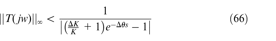
Now, the condition to satisfy for the closed-loop system to be stable is ³⁶

$$||{\Delta }_m(\mathrm{jw})T(\mathrm{jw})||<1\forall \omega \in (-\infty ,\infty )$$

(64)

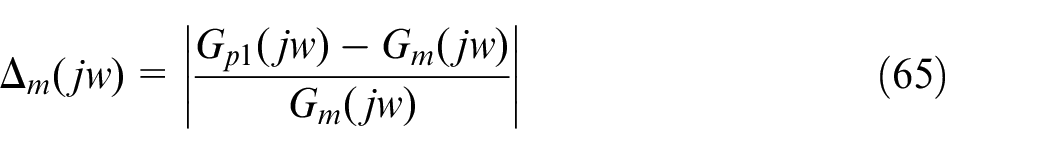
where $T(\mathrm{jw})$ is the complementary sensitivity function, and ${\Delta }_m(\mathrm{jw})$ is the bound on the plant multiplicative uncertainty. The uncertainty in the plant can be expressed as

$${\Delta }_m(\mathrm{jw})=\left|\frac{G_{p1}(\mathrm{jw})-G_m(\mathrm{jw})}{G_m(\mathrm{jw})}\right|$$

(65)

where $G_m(\mathrm{jw})$ is the nominal model that is used for controller design, and $G_{p1}(\mathrm{jw})$ is the actual plant. If uncertainty is present in both the plant gain and dead time, then the tuning parameters have to be selected such that

$$||T(\mathrm{jw})|{|}_{\infty }<\frac{1}{|(\frac{\Delta K}{K}+1)e^{-\Delta \theta s}-1|}$$

(66)

For any integrating model discussed here, the complementary sensitivity function for the proposed scheme is given by

$$T(\mathrm{jw})=\frac{e^{-\mathrm{jw}{\theta }_m}}{\lambda {(\mathrm{jw})}^{\beta }+1}$$

(67)

Also, to ensure robust closed-loop performance, the constraints to be followed by the sensitivity and complementary sensitivity functions are

$$||{\Delta }_m(\mathrm{jw})T(\mathrm{jw})+w_m(\mathrm{jw})(1-T(\mathrm{jw}))||<1$$

(68)

where $w_m(\mathrm{jw})$ is the uncertainty bound on the sensitivity function, which is given as $S(\mathrm{jw})=1-T(\mathrm{jw})$ . Therefore, tuning parameters must be selected so that the resulting controller satisfies the robust performance and stability limitations.

Simulation results

Recent works presented by Siddiqui et al.,^16,37 Raja and Ali, ¹⁵ Çakıroğlu et al., ¹⁴ Jeng, ¹³ Padhan and Majhi, ¹¹ and Uma et al. ¹⁰ were considered for comparative analysis. The response parameters such as rise time $(t_r)$ , settling time ( $t_s$ , s), and integral of time-weighted squared error (ITSE) are calculated to demonstrate performances. A $t_r$ is defined as the time the output takes from 10% to 90% of its steady-state value. The settling time is measured from the output to reach and steady within a given tolerance band. We have considered the 5% band throughout all examples. For evaluating the manipulated input usage, we compute the total variation (TV) in the control signal, which is the sum of all its moves up and down. It is a good measure of the signal’s smoothness and should be as small as possible. If required, a setpoint filter should be added to remove the undesirable overshoot. A low-pass filter of the form $1/(\eta s+1)$ is simple, and parameter $\eta$ is selected appropriately by the designer. ³⁸ The responses and numerical analysis with and without a setpoint filter are shown in all examples. Also, the white noise having a variance of 0.001 is added as a measurement noise to verify the control scheme’s robustness against the noisy output. An extended investigation of the proposed scheme in real-time can be seen from the third example following details from section “The proposed controller design in real-time.”

Example 1

First example is extensively studied in the literature. The outer loop $G_{p1}(s)=2e^{-2s}/s$ and inner loop, $G_{p2}(s)=4e^{-s}/s+1$ are considered as a series plant. Recent method by Siddiqui et al. ¹⁶ presented two types of controllers for the same plant. In a method 1, the primary $G_{c1}(s)=0.06+0.0027/s+0.02s$ and secondary $G_{c2}(s)=0.255+0.212/s$ were suggested. Then, in a method 2, the controllers were taken as $G_{c1}(s)=0.06+0.002s$ and $G_{c2}(s)=0.29+0.17/s$ . Uma et al. ¹⁰ also have studied the same process models with control settings: the primary, $G_{c1}(s)=(1.8+0.5/s+1.93s)[0.5s+1/0.6561s^2+2.960s+1]$ , secondary, $G_{c2}(s)=s+1/2s+4$ , and disturbance rejection controller, $G_{\mathrm{cd}}(s)=(0.0436+.1206s)[0.75s^2+1.5s+1/1.8314s^2+0.7686s+1]$ .

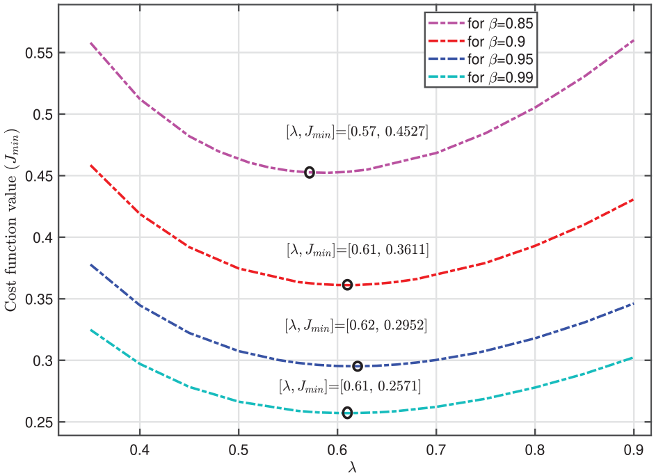
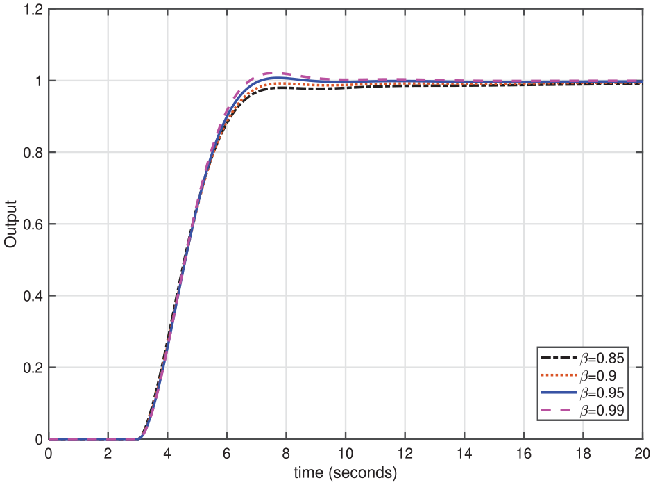
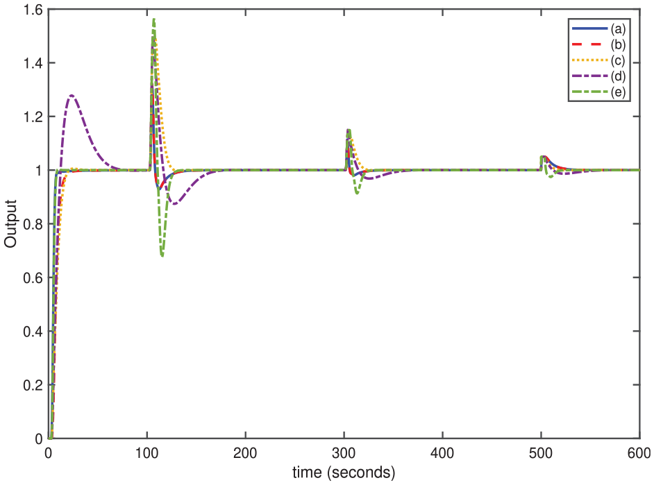
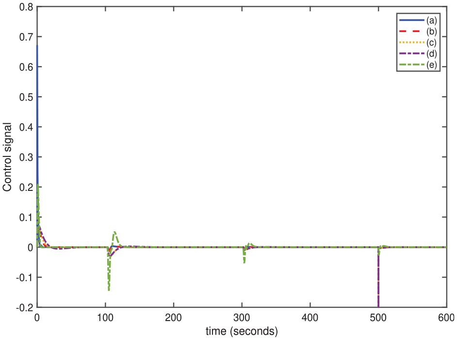
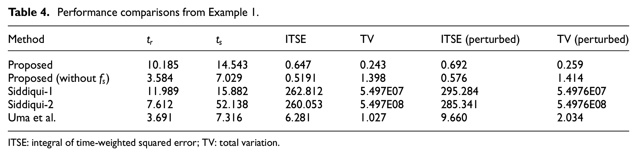
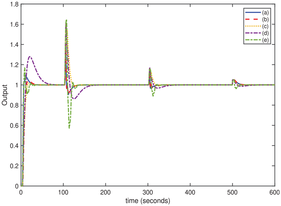
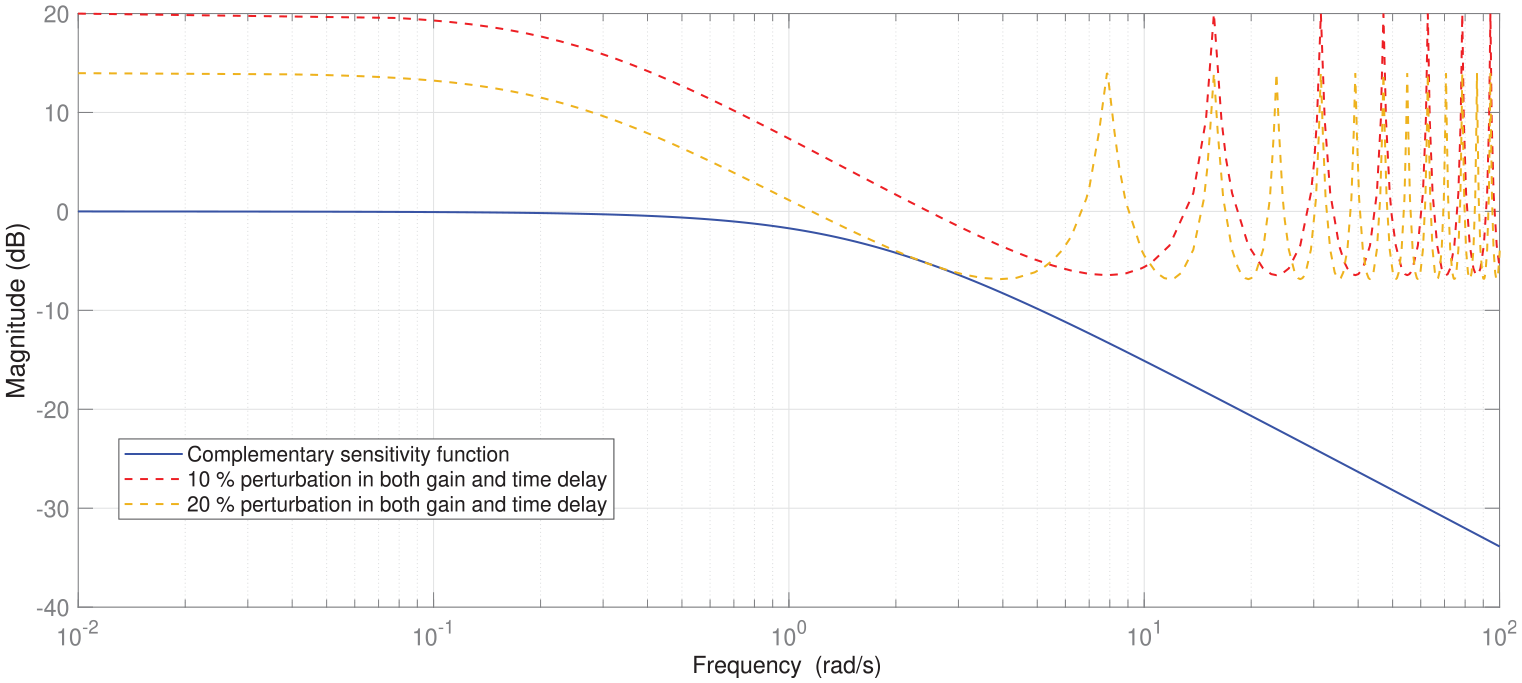
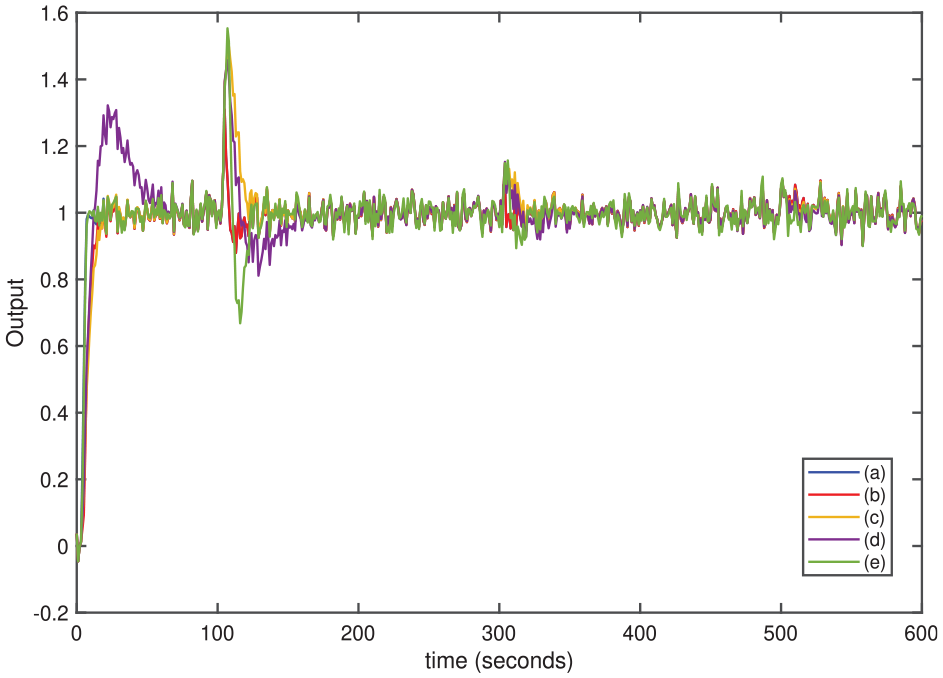
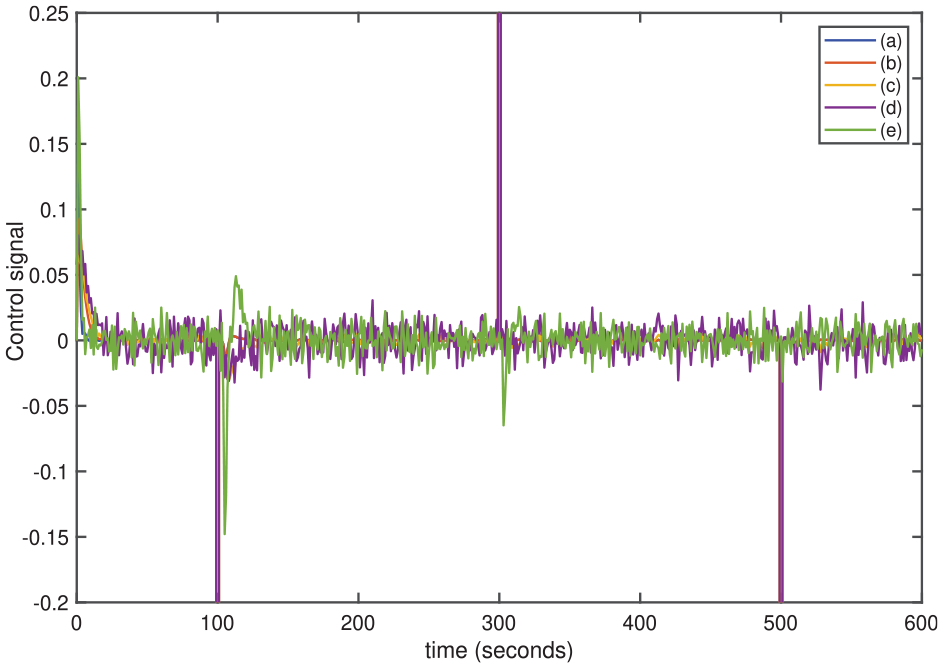
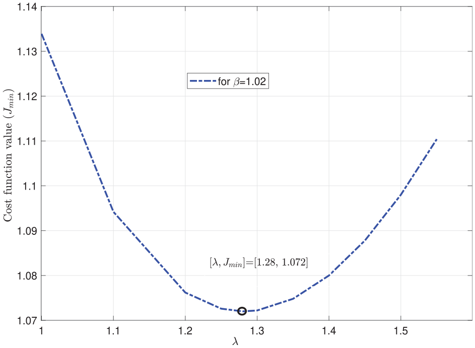
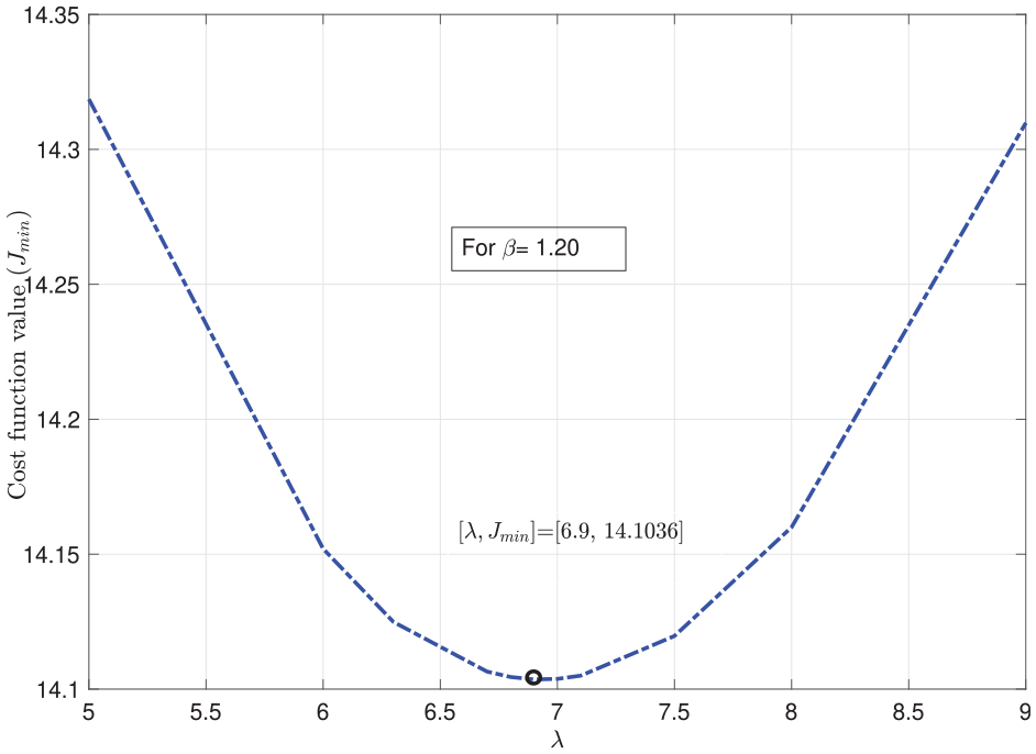
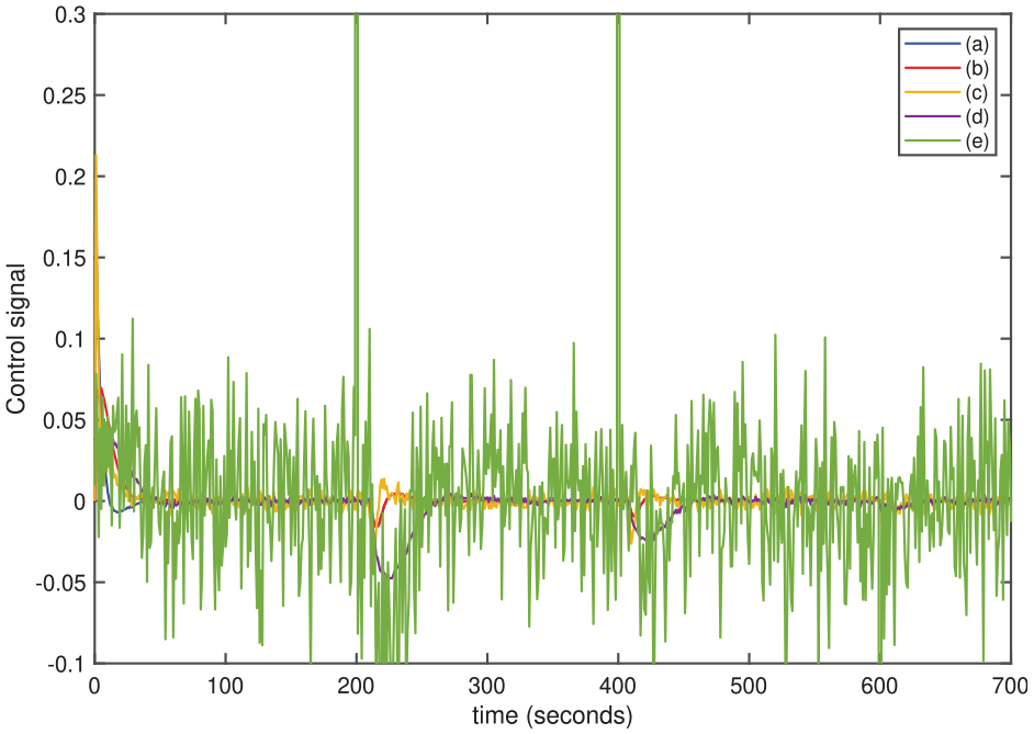
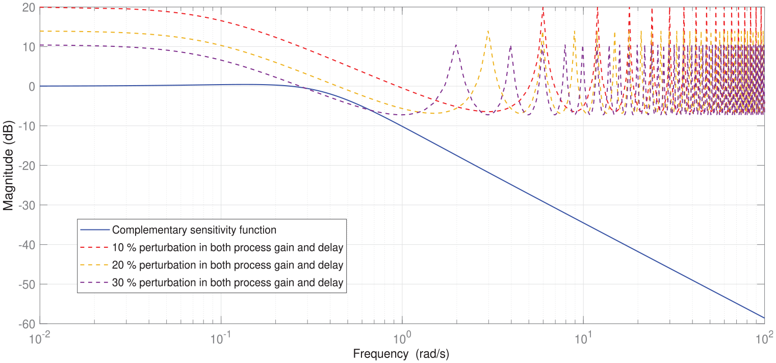
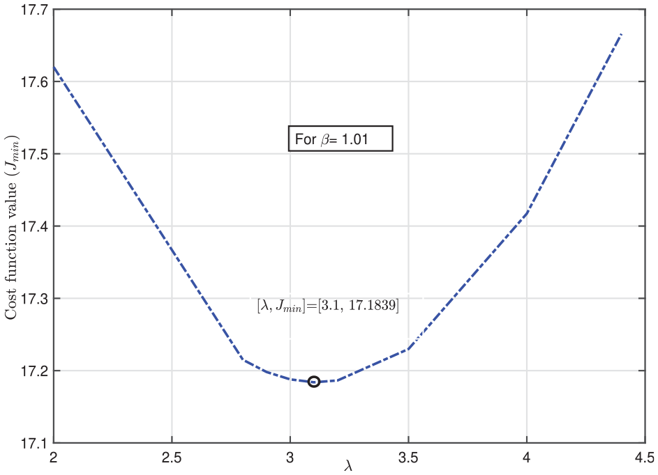
The cost function values with $\beta$ are shown in Figure 5. The corresponding responses are plotted in Figure 6. The results show that one set of parameters is chosen among possible values of $\beta$ to provide the most optimal responses with balanced control performance. Considering this observation, $\beta$ has selected as $0.95$ . The corresponding $g_m$ and ${\varphi }_m$ are $2.3$ and $55.17°$ , respectively. The final controller settings are $K_{c2}=0.125$ , $K_{i2}=0.125$ , and $K_{d1}=0.806$ . The disturbance rejection filter obtained as $F_d=s^2+2s+1/s^2+4s+4$ and that of robustness filter is $F_f(s)=1/8s+1$ . The setpoint filter of the form $f_s=1/(3s+1)$ is also added to improve the setpoint smoothness. A positive load disturbance of $0.05$ is added at 100, 300, and 500 s, respectively. The closed-loop nominal responses and control responses along with other approaches were shown in Figures 7 and 8, respectively. It can be seen the proposed method results a lower overshoot and improved disturbance rejection performances. Table 4 provided the same agreement with the responses by minimum ITSE and TV values. Furthermore, 10% uncertainty is applied in plant parameters gain and delay, in both primary and secondary models. Figure 9 again depicted the robustness from parameter uncertainties. Figure 10 shows the magnitude of the complementary sensitivity function for different perturbations. It is evident that the robust stability margin lowers as perturbation increases, and the controller cannot meet the robust stability requirement stated in equation (66), even with a 20% uncertainty in both gain and time delay. When we tested the methods under the measurement noise with variance = 0.001, Siddiqui et al. ¹⁶ and Uma et al.’s ¹⁰ method obtained large variations in a control signal. The noise test also proved the proposed scheme’s robustness as seen in Figures 11 and 12.

Figure 5.

Calculated cost function values with selected $\beta$ .

Figure 6.

Responses for selected $\beta$ .

Figure 7.

Servo and regulatory responses in Example 1: (a) proposed, (b) proposed with $f_s$ , (c) Siddiqui et al.-1, ¹⁶ (d) Siddiqui et al.–2, ¹⁶ and (e) Uma et al. ¹⁰

Figure 8.

Control signals in Example 1: (a) proposed, (b) proposed with $f_s$ , (c) Siddiqui et al.-1, ¹⁶ (d) Siddiqui et al.-2, ¹⁶ and (e) Uma et al. ¹⁰

Table 4.

Performance comparisons from Example 1.

Method	$t_r$	$t_s$	ITSE	TV	ITSE (perturbed)	TV (perturbed)
Proposed	$10.185$	$14.543$	$0.647$	$0.243$	$0.692$	$0.259$
Proposed (without $f_s$ )	$3.584$	$7.029$	$0.5191$	1.398	$0.576$	$1.414$
Siddiqui-1	$11.989$	$15.882$	$262.812$	$5.497\mathrm{E}07$	$295.284$	$5.4976\mathrm{E}07$
Siddiqui-2	$7.612$	$52.138$	$260.053$	$5.497\mathrm{E}08$	$285.341$	$5.4976\mathrm{E}08$
Uma et al.	$3.691$	$7.316$	$6.281$	$1.027$	$9.660$	$2.034$

ITSE: integral of time-weighted squared error; TV: total variation.

Figure 9.

Perturbed system responses for Example 1: (a) proposed, (b) proposed with $f_s$ , (c) Siddiqui et al.-1, ¹⁶ (d) Siddiqui et al.-2, ¹⁶ and (e) Uma et al. ¹⁰

Figure 10.

Magnitude plot of the complementary sensitivity function for Example 1.

Figure 11.

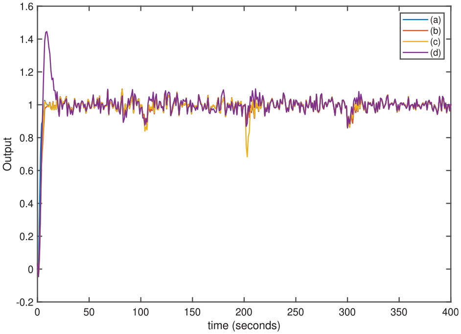
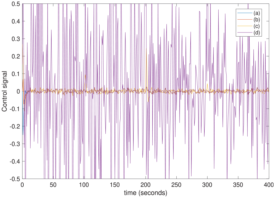
Servo and regulatory responses with measurement noise for Example 1: (a) proposed, (b) proposed with $f_s$ , (c) Siddiqui et al.-1, ¹⁶ (d) Siddiqui et al.-2, ¹⁶ and (e) Uma et al. ¹⁰

Figure 12.

Control responses with measurement noise for Example 1: (a) proposed, (b) proposed with $f_s$ , (c) Siddiqui et al.-1, ¹⁶ (d) Siddiqui et al.-2, ¹⁶ and (e) Uma et al. ¹⁰

Example 2

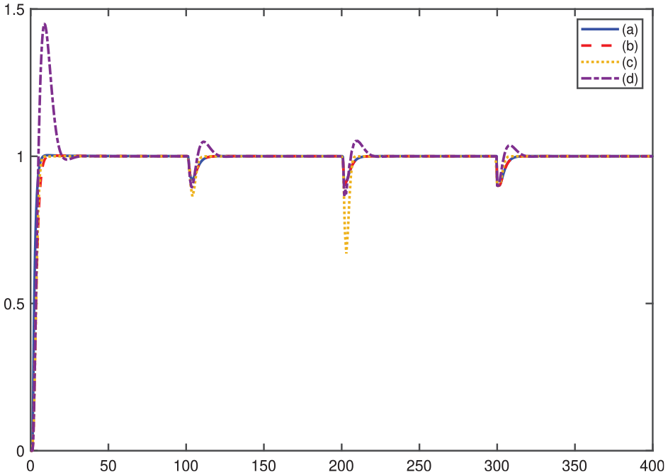
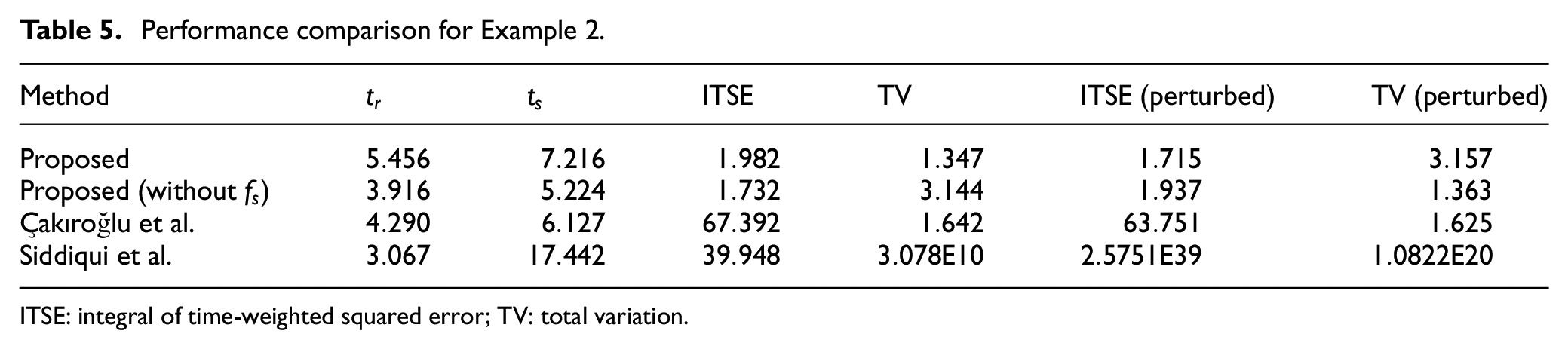
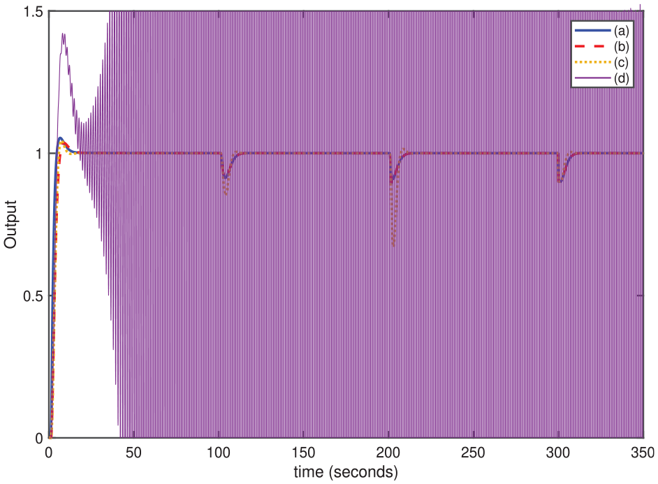
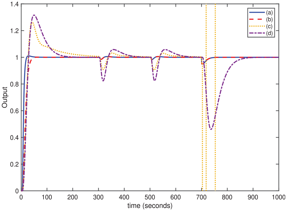
Controlling a double integrating cascading plant is more challenging. A series plant, $G_{p1}(s)=e^{-0.7s}/s^2$ and $G_{p2}(s)=e^{-0.3s}/(s+1)$ was studied by Çakıroğlu et al. ¹⁴ and Siddiqui et al. ¹⁶ In Çakıroğlu et al., ¹⁴ the output decomposition method is presented with two outer-loop controllers, $G_{c1a}(s)=0.833$ and $G_{c1b}(s)=0.333$ , and inner controller as $G_{c2}(s)=3.33s+1/s$ . Whereas in Siddiqui et al., ¹⁶ $G_{c2}=3.74+7.95/s$ and $G_{c1}=0.16+0.02/s+0.56s$ were suggested. After adopting the proposed controller, $\lambda =1.28$ and $\beta =1.02$ are obtained from the chosen $g_m=2.5$ and ${\varphi }_m=52.28°$ . As seen in Figure 13, this choice provided a minimum cost value. Then, the controller parameters are $K_{c2}=1.67$ , $K_{i2}=1.67$ , and $K_{d1}=0.781$ . The setpoint filter $f_s=1/(1.2s+1)$ is added to improve the smoothness of the response. The disturbance rejection filter $F_d=0.3s^2+1.3s+1/0.0225s^2+0.3s+1$ is used in the secondary loop for enhancing disturbance rejection and that of robustness filter is $F_f(s)=1/2.6s+1$ . The step disturbances of magnitude −0.5 are applied at 100 and 200 s, while −0.1 is applied at 300 s. From Figure 14, it is observed that the proposed method shows a similar setpoint response with Çakıroğlu et al. However, the disturbance rejection capability and its control efforts are superior to both methods, seen in Figure 15. Table 5 shows the quantitative analysis for nominal and perturbed models. The lowest values of indices indicate the quality of the proposed method.

Figure 13.

Variation of $\lambda$ and $J_{\min }$ to obtain $\beta$ for Example 2.

Figure 14.

Servo and regulatory responses in Example 2: (a) proposed, (b) proposed with $f_s$ , (c) Çakıroğlu et al., ¹⁴ and (d) Siddiqui et al.-2. ¹⁶

Figure 15.

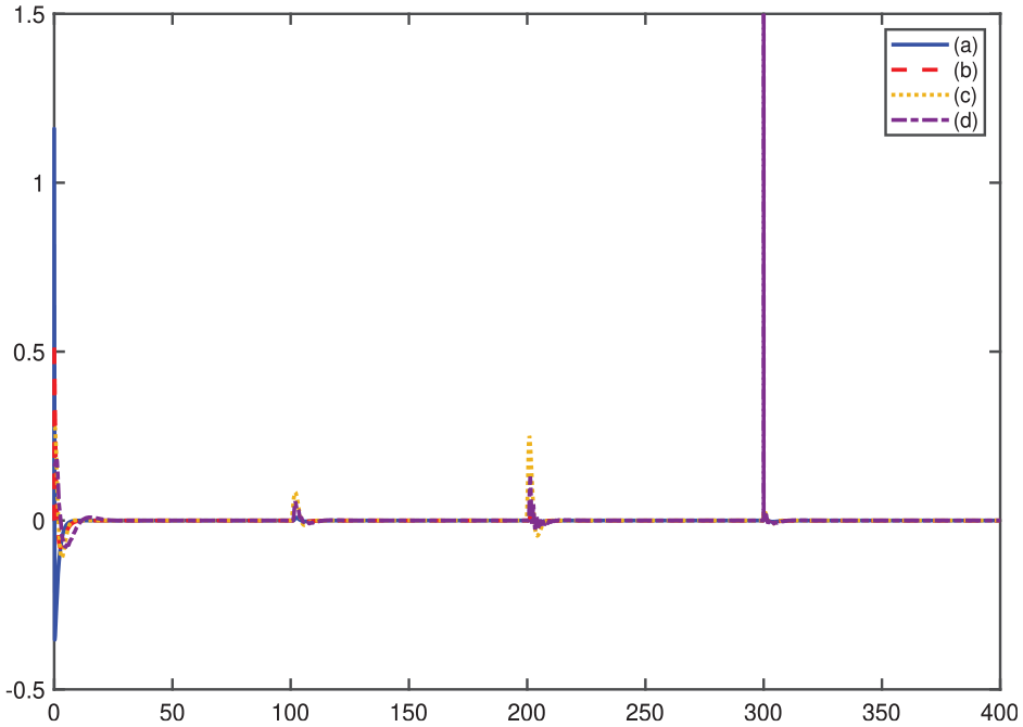
Control signal for Example 2: (a) proposed, (b) proposed with $f_s$ , (c) Çakıroğlu et al., ¹⁴ and (d) Siddiqui et al.-2. ¹⁶

Table 5.

Performance comparison for Example 2.

Method	$t_r$	$t_s$	ITSE	TV	ITSE (perturbed)	TV (perturbed)
Proposed	$5.456$	$7.216$	$1.982$	$1.347$	$1.715$	$3.157$
Proposed (without $f_s$ )	$3.916$	$5.224$	$1.732$	$3.144$	$1.937$	$1.363$
Çakıroğlu et al.	$4.290$	$6.127$	$67.392$	$1.642$	$63.751$	$1.625$
Siddiqui et al.	$3.067$	$17.442$	$39.948$	$3.078\mathrm{E}10$	$2.5751\mathrm{E}39$	$1.0822\mathrm{E}20$

ITSE: integral of time-weighted squared error; TV: total variation.

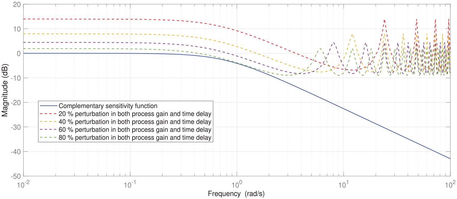
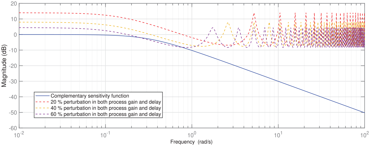
Furthermore, the perturbations test with 10% changes in gain and time delay for both primary and secondary plants is shown in Figure 16. One can see that Siddiqui et al. method failed the perturbation test. From Figure 17, it can be inferred that the maximum permitted perturbation is 70% because any additional rise in perturbation causes output from the system to become excessively oscillatory. When we tested the methods under the measurement noise with variance = 0.001, Siddiqui et al.’s ¹⁶ method obtained large variations in a control signal. The noise test also proved the proposed scheme’s robustness as per Figures 18 and 19.

Figure 16.

Perturbed system responses for Example 2: (a) proposed, (b) proposed with $f_s$ , (c) Çakıroğlu et al., ¹⁴ and (d) Siddiqui et al.-2. ¹⁶

Figure 17.

Magnitude plot of the complementary sensitivity function for Example 2.

Figure 18.

Servo and regulatory responses with measurement noise for Example 2: (a) proposed, (b) proposed with $f_s$ , (c) Çakıroğlu et al., ¹⁴ and (d) Siddiqui et al.-2. ¹⁶

Figure 19.

Control responses with measurement noise for Example 2: (a) proposed, (b) proposed with $f_s$ , (c) Çakıroğlu et al., ¹⁴ and (d) Siddiqui et al.-2. ¹⁶

Example 3

A large time delay cascade integrating plant, with $G_{p1}(s)=e^{-6.5672s}/s(3.4945s+1)$ and $G_{p2}(s)=2e^{-2s}/s+1$ studied by Raja and Ali. ¹⁵ They have applied a series-cascade control with inner and outer loops as classical PIs. The parameter settings were $K_{c1}=0.039$ , $T_{i1}=845.34$ , $K_{c2}=0.2717$ , and $T_{i2}=1.656$ . Also, a stabilizing proportional controller, $K_p=0.0012$ was added in the structure. For the same plant, Padhan and Majhi ¹¹ designed two controllers and a setpoint filter. They have given, a setpoint filter $6.989s^3+5.4945s^2+s+1/628.806s^3+220.1907s^2+25.7016s+1$ , inner-loop controller, $G_{c2}=s+1/4s+2$ , and outer-loop disturbance rejection controller with lead-lag compensator, $G_{c3}=0.0456(1+1/61.9704s+1.9355s)(42.7476s^3+32.1915s^2+9.2060s+1/45.3194s^3+29.0943s^2+7.8726s+1)$ . As it could be seen that their method suggested a higher-order function.

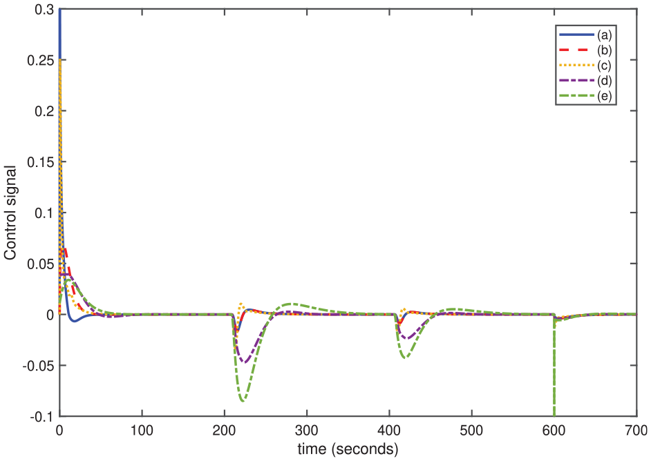
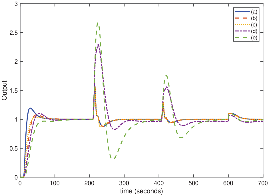
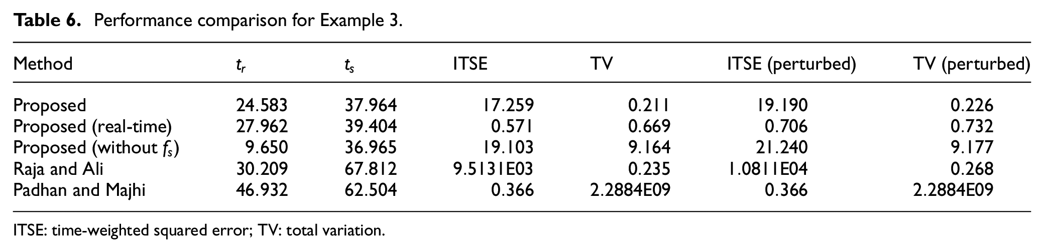
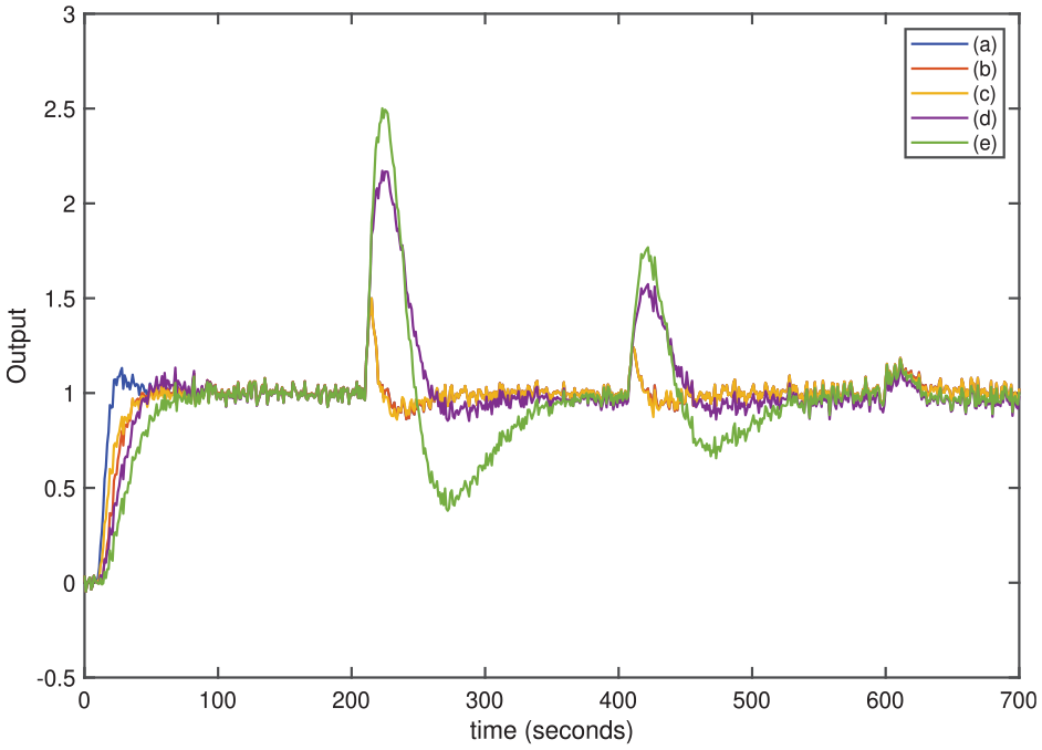
For the same plant, our method suggested a fractional controller with ${\varphi }_m=53.16°$ and $g_m=5$ . Following the design steps, we have obtained parameters $\lambda =3.38$ and $\beta =1.2$ . Figure 20 presents the index value with chosen $\lambda$ and $\beta$ values. Then, the inner-loop and outer-loop parameters become $K_{c2}=0.125$ , $K_{i2}=0.125$ , $K_{i1}=0.145$ , and $K_{d1}=0.506$ . From Table 2, the TID controller values can be obtained based on minimum cost index value $\lambda =1$ , as $K_{t1}=0.01$ , $K_{i1}=1.03$ , and $K_{d1}=3.494$ . The disturbance rejection filter $F_d=2s^2+3s+1/2s^2+4s+2$ and that of robustness filter is $F_f(s)=1/21.1344s+1$ . The disturbance inputs are considered with a magnitude of $0.2$ at $t=200\mathrm{s}$ , at $t=400\mathrm{s}$ and $0.1$ at $t=600\mathrm{s}$ . The servo and regulatory responses and control efforts are shown in Figures 21 and 22, respectively. The setpoint filter of the form $f_s=1/(10s+1)$ is added to improve smoothness of response. To illustrate the robustness test, perturbation of 10% in the time delay and plant gain of both primary and secondary plants have been considered at once and shown in Figure 23. From the numerical analysis shown in Table 6, it is observed that the output obtains the desired setpoint value quickly with minimum TV and optimal ITSE values. In general, the closed-loop responses from the proposed method are superior to the improved load disturbance rejections. The outputs and control variations with measurement noise in Figures 24 and 25 show that Padhan and Majhi’s method shows more control variations compared to others. In addition to performance analysis, robustness stability analysis for the proposed scheme has also been done and is shown in Figure 26.

Figure 20.

Variation of $\lambda$ and $J_{\min }$ to obtain $\beta$ for Example 3.

Figure 21.

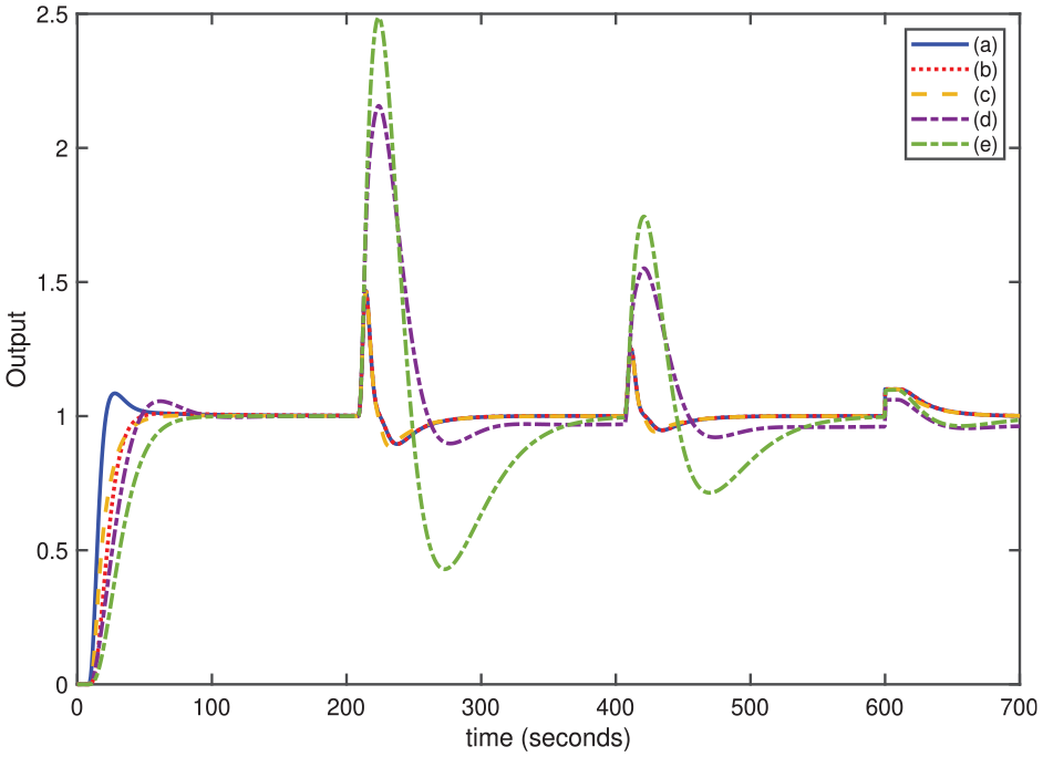
Servo as well as regulatory responses for Example 3: (a) proposed, (b) proposed with $f_s$ , (c) proposed (real-time), (d) Raja and Ali, ¹⁵ and (e) Padhan and Majhi. ¹¹

Figure 22.

Control signal for Example 3: (a) proposed, (b) proposed with $f_s$ , (c) proposed (real-time), (d) Raja and Ali, ¹⁵ and (e) Padhan and Majhi. ¹¹

Figure 23.

Perturbed system responses for Example 3: (a) proposed, (b) proposed with $f_s$ , (c) proposed (real-time), (d) Raja and Ali, ¹⁵ and (e) Padhan and Majhi. ¹¹

Table 6.

Performance comparison for Example 3.

Method	$t_r$	$t_s$	ITSE	TV	ITSE (perturbed)	TV (perturbed)
Proposed	$24.583$	$37.964$	$17.259$	$0.211$	$19.190$	$0.226$
Proposed (real-time)	$27.962$	$39.404$	$0.571$	$0.669$	$0.706$	$0.732$
Proposed (without $f_s$ )	$9.650$	$36.965$	$19.103$	$9.164$	$21.240$	$9.177$
Raja and Ali	$30.209$	$67.812$	$9.5131\mathrm{E}03$	$0.235$	$1.0811\mathrm{E}04$	$0.268$
Padhan and Majhi	$46.932$	$62.504$	$0.366$	$2.2884\mathrm{E}09$	$0.366$	$2.2884\mathrm{E}09$

ITSE: time-weighted squared error; TV: total variation.

Figure 24.

Servo and regulatory responses with measurement noise for Example 3: (a) proposed, (b) proposed with $f_s$ , (c) proposed (real-time), (d) Raja and Ali, ¹⁵ and (e) Padhan and Majhi. ¹¹

Figure 25.

Control responses with measurement noise for Example 3: (a) proposed, (b) proposed with $f_s$ , (c) proposed (real-time), (d) Raja and Ali, ¹⁵ and (e) Padhan and Majhi. ¹¹

Figure 26.

Magnitude plot of the complementary sensitivity function for Example 3.

Example 4

A higher-order integrating plant with $G_{p1}(s)=e^{-3s}/s(10s+1)(2s+1)$ and $G_{p2}(s)=e^{-0.5s}/s+1$ studied by Siddiqui et al. ³⁷ and Jeng. ¹³ Jeng suggested a master controller with parameters as $K_{c1}=0.0862$ , $T_{i1}=56.34$ , and $T_{d1}=8.50$ and slave controller as $K_{c2}=1.336$ and $T_{i2}=0.833$ . Siddiqui et al. suggested secondary controller settings as $G_{c2}(s)=2.68+2.81/s+0.45s$ and primary controller settings as $G_{c2}(s)=0.1+0.001/s+0.65s$ . ³⁷

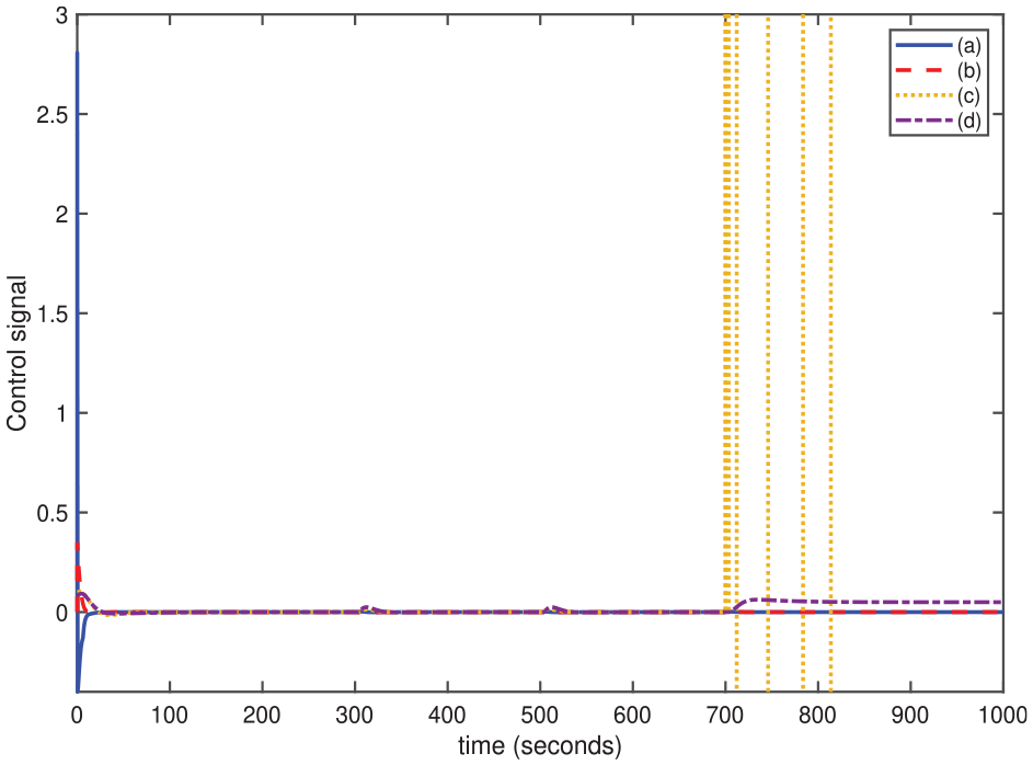
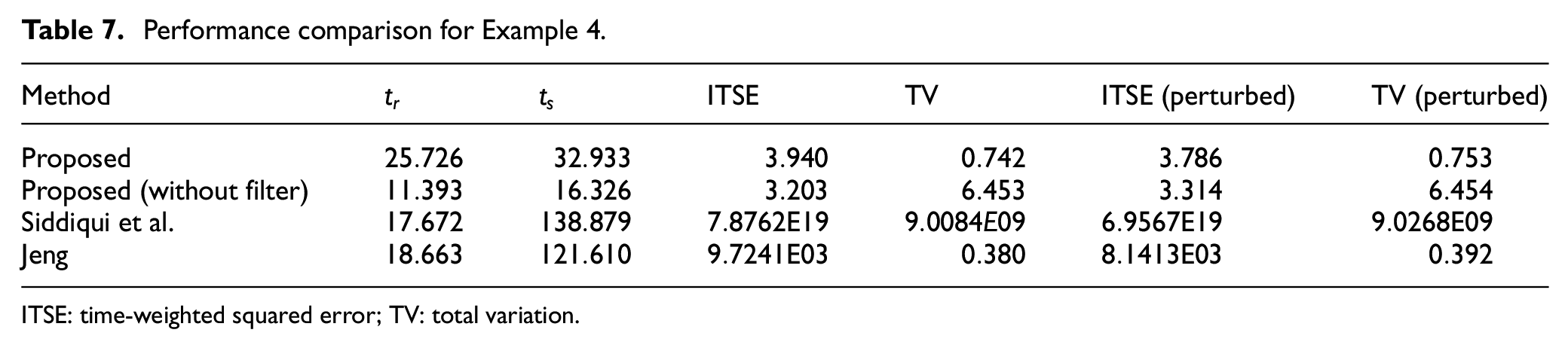
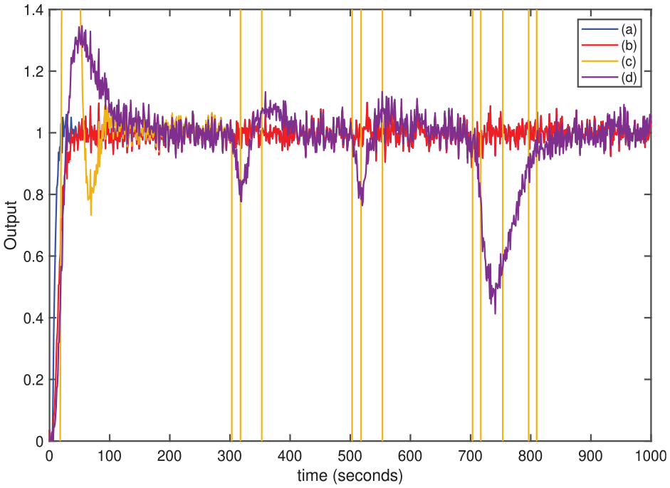
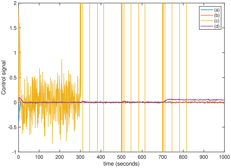
Now, the proposed method designs the fractional IMC filter using ${\varphi }_m=59.07°$ and $g_m=3$ . Following the procedure, we have obtained $\lambda =3.1$ and $\beta =1.01$ as per values from Figure 27. The controller settings are $K_{p2}=1.0$ , $K_{i2}=1.0$ , $K_{i1}=0.323$ , and $K_{d1}=3.226$ . The setpoint filter $f_s=1/(8s+1)$ , the robustness filter $F_f(s)=1/12s+1$ , and the disturbance filter $F_d=0.5s^2+1.5s+1/0.0625s^2+0.5s+1$ are included as per the structure. The closed-loop responses under the presence of disturbances −0.5 at 300 and 500 s and −0.05 at 700 s are shown in Figure 28. The corresponding control signals are plotted in Figure 29. For encapsulating the system robustness, a perturbation of 10% is introduced in gain and dead time of $G_{p2}$ and $G_{p1}$ . The test results are given in Figure 30 with other methods’ performance. The numerical values are measured and listed in Table 7. From these results, it can be proven that the new fractional IMC with SP structure provides better tracking and robustness in comparison to the recent literature method. When we test the methods with measurement noise as shown in Figures 31 and 32, the Siddiqui et al.’s ³⁷ method again shows worst performance and large variations in the control signal. It can be noticed from Figure 33 that maximum allowable perturbation is allowable up to 50%.

Figure 27.

Variation of $\lambda$ and $J_{\min }$ to obtain $\beta$ for Example 4.

Figure 28.

Servo as well as regulatory responses for Example 4: (a) proposed, (b) proposed with $f_s$ , (c) Siddiqui et al., ³⁷ and (d) Jeng et al. ¹³

Figure 29.

Control signal for Example 4: (a) proposed, (b) proposed with $f_s$ , (c) Siddiqui et al., ³⁷ and (d) Jeng et al. ¹³

Figure 30.

Perturbed system responses for Example 4: (a) proposed, (b) proposed with $f_s$ , (c) Siddiqui et al., ³⁷ and (d) Jeng et al. ¹³

Table 7.

Performance comparison for Example 4.

Method	$t_r$	$t_s$	ITSE	TV	ITSE (perturbed)	TV (perturbed)
Proposed	$25.726$	$32.933$	$3.940$	$0.742$	$3.786$	$0.753$
Proposed (without filter)	$11.393$	$16.326$	$3.203$	$6.453$	$3.314$	$6.454$
Siddiqui et al.	$17.672$	$138.879$	$7.8762\mathrm{E}19$	$9.0084E09$	$6.9567\mathrm{E}19$	$9.0268\mathrm{E}09$
Jeng	$18.663$	$121.610$	$9.7241\mathrm{E}03$	$0.380$	$8.1413\mathrm{E}03$	$0.392$

ITSE: time-weighted squared error; TV: total variation.

Figure 31.

Servo and regulatory responses with measurement noise for Example 4: (a) proposed, (b) proposed with $f_s$ , (c) Siddiqui et al., ³⁷ and (d) Jeng et al. ¹³

Figure 32.

Control responses with measurement noise for Example 4: (a) proposed, (b) proposed with $f_s$ , (c) Siddiqui et al., ³⁷ and (d) Jeng et al. ¹³

Figure 33.

Magnitude plot of the complementary sensitivity function for Example 4.

Conclusion

This article developed a hybrid structure with IMC and SP concepts for integrating plants with time delay. The suggested method includes the fractional-order IMC filter, having an additional degree for improving performance. This design is simple, with two tuning parameters, which follow good robustness under significant disturbance inputs and parameter perturbation. Moreover, a selection task becomes manageable using the balanced cost function and margins ( $g_m$ , ${\varphi }_m$ ) relationship. The system’s performance can be implemented in all classes of integrating plants, including third-order plants in the outer loop. Quantitative analysis is carried out using ITSE and TV, and the proposed method shows promising results compared to previous works with the same or more tuning parameters. As one can see, there is no or minimal overshoot even without a setpoint filter, which is the key advantage compared to other approaches. The designer can choose the setpoint value so that desired response concerning settling time and rise time can be accomplished. Using the proposed controllers, simulation results show robust stability, better control performance, and disturbance rejection.

Now, research is underway to extend the proposed method to fractional-order integrating plant models and other types of plants with unstable and positive/negative zeroes. Research can be done to develop a fractional controller for plants with delay, even though the SP makes the system complex. Future research can also be conducted for series-cascade unstable models and the related extension of the proposed methodology. The authors believe that the method will provide a considerable effort toward fractional-order control in industrial use.