Event-driven adaptive intermittent control applied to a rotational pendulum

Abstract

Intermittent control combines open-loop trajectories with feedback at discrete time instances determined by events. Among other applications, it has recently been used to model quiet standing in humans where the system was assumed to be time-invariant. This article expands this work to the time-variant case by introducing an adaptive intermittent controller that exploits the well-known self-tuning architecture of adaptive control with a Kalman filter to perform online state and parameter estimation. Simulation and experimental results using a rotational inverted pendulum show advantages of the intermittent controllers compared to continuous feedback control since the former can provide persistent excitation due to their internal triggering mechanism, even when no external reference changes or disturbances are applied. Moreover, the results show that the event thresholds of intermittent control can be used to adjust the degree of responsiveness of the adaptation in the system, becoming a tool to balance the trade-off between steady-state performance and flexibility against parametric changes, addressing the stability–plasticity dilemma of adaptation and learning in control.

Introduction

Event-driven intermittent control (IC)^1–4 has been proposed as a model that explains the underlying control mechanisms of human balance. At its core, the fundamental property of alternating between open- and closed-loop configurations provides two main advantages: (1) the open-loop evolution reduces the overall bandwidth of the controller while providing resources to perform state-dependant optimisation ⁵ and (2) serves as a mechanism to modulate the relationship between exploration and exploitation or, in other words, the stability and plasticity trade-off that is critical for adaptation and learning. ⁶ While IC has been used in the physiological control context,^7–12 its engineering origins come from the practical implementation of model-based predictive control (MPC) in the presence of hard constraints ¹³ and the observer-predictor-feedback architecture, ¹⁴ supported by experimental results on physical real-time systems.^15,16 While a variety of different IC implementations exist, ³ the form of IC considered in this article relies on the principle of continuous observation and intermittent action, meaning that the states are monitored all the time, but only used to recalculate the control signal at discrete points in time (or events) which are determined by a triggering mechanism. Between events, the controller applies an open-loop control signal that is generated by a generalised hold and evolves using its own internal states. When an event occurs, the controller uses observed states instead to produce a new control signal for the next open-loop interval.

IC has been extended recently to include the multivariable case, with an emphasis on multi-link unstable models of human standing,^4,6,17 where it has been argued that the open-loop intervals and the impulse-like control signals in IC could benefit adaptive schemes in situations where model uncertainties are present or when the system parameters vary with time. This is based on the idea that the variability caused by the open-loop interval results in events and corresponding control actions that excite the system more often than a controller with less sensorimotor variability, facilitating system identification. This hypothesis was tested in the context of human control,^18,19 verifying that an intermittent strategy allowed subjects controlling a virtual inverted pendulum with a joystick to perform better against parameter variations compared to subjects that used a continuous strategy. Gawthrop et al. ⁴ applied adaptive intermittent controllers to simulate human balance control in single-input single-output scenarios, using a formulation that solved the online identification problem via state-variable filters, using a non-minimal state-space representation of the system. A self-tuning architecture was used,^20,21 which separates the algorithm in an online system identification stage followed by a controller redesign.

In this article, an adaptive intermittent controller is introduced by combining joint Kalman filters that perform online state and parameter estimation in a single routine, using the aforementioned self-tuning architecture. In addition, this controller uses a closed-loop representation of the overall system dynamics to generate open-loop control trajectories and is based on earlier initial results. ²² This particular type of hold is known as the system-matched hold, ²³ and it provides a reference model of the ideal behaviour of the system under the influence of a control signal. The framework is not limited to this type of hold; for instance, an intermittent tapping hold ²⁴ could be incorporated to produce the inter-sample behaviour. In IC, an event triggers the use of the observer states for feedback; however, since the joint Kalman filter also estimates a vector of time-varying parameters, these values are used to recalculate the different components of the intermittent controller before applying the final control law, providing an adaptation layer to IC.

The next section of the article introduces our adaptive IC architecture. Thereafter, the simulation results are presented, followed by experimental results, leading to the conclusions drawn from this work.

Continuous control

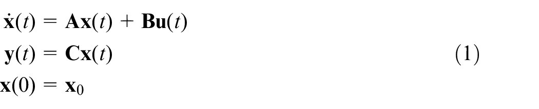
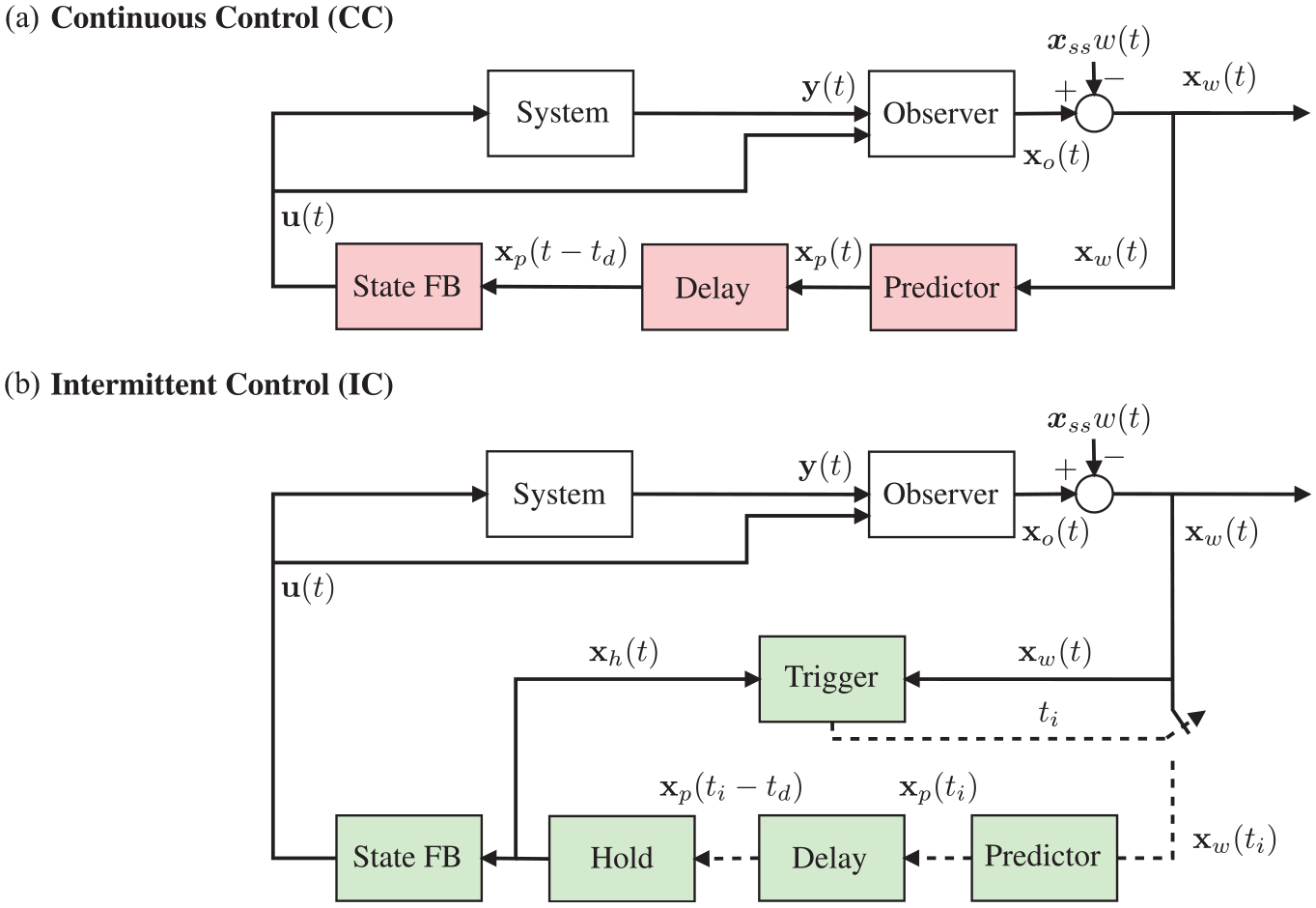
The adaptive intermittent controller presented in this article is based on a continuous predictive controller (CC) which is shown in Figure 1(a). This model assumes that the controlled system can be written as a linear state-space model of order n, as follows

$$\begin{array}{c}\multicolumn{1}{c}{\stackrel{·}{\mathbf{x}}(t)=\mathbf{Ax}(t)+\mathbf{Bu}(t)}\\ \multicolumn{1}{c}{\mathbf{y}(t)=\mathbf{Cx}(t)}\\ \multicolumn{1}{c}{\mathbf{x}(0)={\mathbf{x}}_0}\end{array}$$

(1)

where $\mathbf{x}\in {\mathbb{R}}^n$ , $\mathbf{y}\in {\mathbb{R}}^{n_y}$ , and $\mathbf{u}\in {\mathbb{R}}^{n_u}$ are the system state, output, and input, respectively, and $t$ corresponds to continuous time. $\mathbf{A}$ is a matrix with a dimension of $n\times n$ , $\mathbf{B}$ is $n\times n_u$ , $\mathbf{C}$ is $n_y\times n$ , and ${\mathbf{x}}_0$ is an $n\times 1$ vector of initial conditions. The dynamical model in equation (1) is represented in the diagram by the block labelled as System. The Observer estimates the system states ${\mathbf{x}}_o(t)$ continuously, which are passed to the rest of the structures in the feedback loop after a reference input $w(t)$ is introduced to generate ${\mathbf{x}}_w(t)={\mathbf{x}}_o(t)-{\mathit{x}}_{\mathrm{ss}}w(t)$ . The steady-state component ${\mathit{x}}_{\mathrm{ss}}$ is calculated offline, and it is part of the design process described in the next section. The Predictor compensates for possible delays in the loop by generating the future states ${\mathbf{x}}_p(t)$ . To generate a control law that stabilises equation (1), we could resort to an underlying continuous design (UCD) stage, which involves the design of a state-feedback controller, state prediction, and the introduction of steady-state components.

Figure 1.

Continuous and intermittent control: (a) the continuous observer-predictor-feedback model ¹⁴ serves as the basis for IC. The quantities $\mathbf{y}(t)$ , $\mathbf{u}(t)$ , and $w(t)$ represent outputs, inputs, and reference, respectively. The product ${\mathit{x}}_{\mathrm{ss}}w(t)$ is the vector version of $w(t)$ , and the observed states are defined by ${\mathbf{x}}_o(t)$ . The Predictor generates future states ${\mathbf{x}}_p(t_i)$ to compensate for the time-delay $t_d$ . The state-feedback block labelled as State FB represents the gains that are used to compute the control input $\mathbf{u}(t)$ continuously.(b) IC uses a Hold to produce internal states ${\mathbf{x}}_h(t)$ which are compared against ${\mathbf{x}}_w(t)$ by a Trigger mechanism. If the difference exceeds a predefined threshold $q$ , then an event is created at time $t_i$ . The hold states ${\mathbf{x}}_h(t)$ are used to compute the control signal $\mathbf{u}(t)$ between events which evolves in an open-loop configuration, until it is reset at times $t_i$ by the Predictor. The dashed lines represent quantities that are defined only at event times.

Underlying continuous design

A state-feedback controller with gain $\mathbf{k}$ is used to formulate a control law of the form

$$\mathbf{u}(t)=-\mathbf{k}{\mathbf{x}}_p(t-t_d)+{\mathit{u}}_{\mathrm{ss}}w(t)$$

(2)

which is used to stabilise the system in equation (1). Here, $w(t)$ is an external reference signal, $t_d$ is a constant time-delay, and ${\mathbf{x}}_p(t)$ is the predicted state vector at time $t+t_d$ based on the data available at time $t$ .^2,14 The delay $t_d$ can be included to account for transmission and computational delays in the human operator, which is an assumption derived from human motor control and physiology. ² This implies that the delay is part of the controller in the feedback loop.

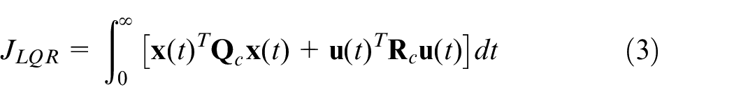
A standard linear quadratic regulator (LQR) approach ²⁵ is used to obtain $\mathbf{k}$ , this involves the minimisation of the LQR cost function

$$J_{\mathrm{LQR}}={\int }_0^{\infty }[\mathbf{x}{(t)}^T{\mathbf{Q}}_c\mathbf{x}(t)+\mathbf{u}{(t)}^T{\mathbf{R}}_c\mathbf{u}(t)]\mathrm{dt}$$

(3)

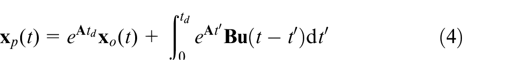
and the solution of its associated algebraic Riccati equation. Both $\mathbf{x}(t)$ and $\mathbf{u}(t)$ in equation (3) are weighted by the diagonal design matrices ${\mathbf{Q}}_c$ (an $n\times n$ matrix that must be positive semi-definite) and ${\mathbf{R}}_c$ (an $n_u\times n_u$ positive definite matrix). The state vector ${\mathbf{x}}_p(t)$ used in equation (2) is calculated via a state-predictor of the following form

$${\mathbf{x}}_p(t)=e^{\mathbf{A}{t}_d}{\mathbf{x}}_o(t)+{\int }_0^{t_d}{e}^{\mathbf{A}t\prime }\mathbf{Bu}(t-t\prime )\mathrm{d}t\prime$$

(4)

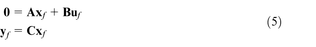
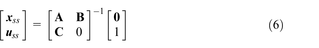
The reference $w(t)$ is introduced by considering that the system has reached the steady-state

$$\begin{array}{c}\multicolumn{1}{c}{0=\mathbf{A}{\mathbf{x}}_f+\mathbf{B}{\mathbf{u}}_f}\\ \multicolumn{1}{c}{{\mathbf{y}}_f=\mathbf{C}{\mathbf{x}}_f}\end{array}$$

(5)

where ${\mathbf{x}}_f$ , ${\mathbf{u}}_f$ , and ${\mathbf{y}}_f$ are the steady-state versions of the states, inputs, and outputs, respectively. The goal is to ensure that ${\mathbf{y}}_f=w(t)$ at all times, which can be achieved by substituting the expressions ${\mathbf{x}}_f={\mathit{x}}_{\mathrm{ss}}w(t)$ and ${\mathbf{u}}_f={\mathit{u}}_{\mathrm{ss}}w(t)$ in equation (5) and cancelling the common factor $w(t)$ , resulting in the following system from which ${\mathit{x}}_{\mathrm{ss}}$ and ${\mathit{u}}_{\mathrm{ss}}$ can be obtained

$$\left[\begin{array}{c}{\mathit{x}}_{\mathrm{ss}}\hfill \\ \multicolumn{1}{c}{{\mathit{u}}_{\mathrm{ss}}}\end{array}\right]={\left[\begin{array}{cc}\mathbf{A}\hfill & \mathbf{B}\hfill \\ \multicolumn{1}{c}{\mathbf{C}}& 0\hfill \end{array}\right]}^{-1}\left[\begin{array}{c}0\hfill \\ \multicolumn{1}{c}{1}\end{array}\right]$$

(6)

Both ${\mathit{x}}_{\mathrm{ss}}\mathrm{equation}$ and ${\mathit{u}}_{\mathrm{ss}}$ can be computed offline.

Intermittent control

The general IC architecture,^2,4,16 shown in Figure 1(b), builds up on the previously introduced CC by adding two fundamental components: The generalised Hold uses the predicted states ${\mathbf{x}}_p(t_i)$ to create an open-loop hold state ${\mathbf{x}}_h$ , which is used to calculate the control trajectories via the state-feedback gain $\mathbf{k}$ . These control trajectories are applied between the events imposed by the Trigger mechanism at discrete points in time $t_i$ . The trigger mechanism involves continuously comparing the Predictor states ${\mathbf{x}}_p(t)$ with the state and ${\mathbf{x}}_w(t)$ triggering an event if the difference between them exceeds a predefined threshold $q$ . This action closes the feedback loop at $t_i$ .

Intermittent control time frames

The different time frames that are used in IC are defined as follows:

1. Continuous time $(t)$ : time that describes the system evolution.

2. Discrete-time $(t_i)$ : instances of time that indicate when an event has been generated, shown as subscript i. The elapsed time between consecutive events is the intermittent interval ${\Delta }_i^{\mathrm{ol}}=t_{i+1}-t_i$ .

3. Intermittent-time $(\tau )$ : when an event is generated at $t_i$ , the continuous-time variable $\tau$ is reset using $\tau =t-t_i$ . A lower limit ${\Delta }_{\min }^{\mathrm{ol}}>0$ is established for every intermittent interval such that ${\Delta }_i^{\mathrm{ol}}>{\Delta }_{\min }^{\mathrm{ol}}$ . The lower limit ${\Delta }_{\min }^{\mathrm{ol}}$ is commonly known as the minimum open-loop interval.

The system-matched hold

The open-loop behaviour of IC is dictated by the states that the hold produces, which are used to generate a control input of the following form

$$\mathbf{u}(t)=-\mathbf{k}{\mathbf{x}}_h(\tau )+{\mathit{u}}_{\mathrm{ss}}w(t)$$

(7)

where ${\mathbf{x}}_h$ are the hold states, which evolve in time according to $\tau$ , with dynamics generated by an autonomous system as follows

$${\stackrel{·}{\mathbf{x}}}_h(\tau )={\mathbf{A}}_h{\mathbf{x}}_h(\tau )$$

(8)

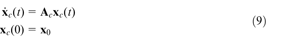
The dynamics of equation (8) are determined by ${\mathbf{A}}_h$ . To produce hold states that are an approximation of the real system states (in the absence of disturbances or noise), ${\mathbf{A}}_h$ can be matched to the behaviour of an ideal delay-free closed-loop system of the following form

$$\begin{array}{c}\multicolumn{1}{c}{{\stackrel{·}{\mathbf{x}}}_c(t)={\mathbf{A}}_c{\mathbf{x}}_c(t)}\\ \multicolumn{1}{c}{{\mathbf{x}}_c(0)={\mathbf{x}}_0}\end{array}$$

(9)

with dynamics dictated by the closed-loop matrix ${\mathbf{A}}_c=\mathbf{A}-\mathbf{Bk}$ . This choice of hold, where ${\mathbf{A}}_h={\mathbf{A}}_c$ , is known as the system-matched hold ²³ and provides a suitable reference model for the detection of trigger events. Its simplicity makes it particularly attractive from an implementation point of view, and for this reason, it has been used widely to implement intermittent controllers. Alternative versions are also possible, such as the tapping hold. ²⁴

At the start of each intermittent interval, $t=t_i$ , the hold states are reset to the predicted state

$${\mathbf{x}}_h(t_i)={\mathbf{x}}_p(t_i-t_d)$$

(10)

Details on how to obtain the predicted states ${\mathbf{x}}_p$ in an intermittent context are given in the following section.

Intermittent prediction

To compensate for a possible time-delay $t_d$ , the following dynamical system, based on the system matrices from equation (1), can be established during the intermittent time frame $\tau$

$${\stackrel{·}{\mathbf{x}}}_p(\tau )=\mathbf{A}{\mathbf{x}}_p(\tau )+\mathbf{Bu}(\tau )\mathrm{with}{\mathbf{x}}_p(0)={\mathbf{x}}_w(t_i)$$

(11)

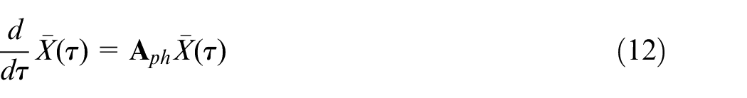
and evaluated at $\tau =t_d$ . Combining equations (11) and (8) yields the following extended system

$$\frac{d}{d\tau }\overline{X}(\tau )={\mathbf{A}}_{\mathrm{ph}}\overline{X}(\tau )$$

(12)

$$\overline{X}(0)={\overline{X}}_i$$

(13)

$${\mathbf{A}}_{\mathrm{ph}}=\left[\begin{array}{cc}\mathbf{A}\hfill & -\mathbf{Bk}\hfill \\ \multicolumn{1}{c}{0_{n\times n}}& {\mathbf{A}}_h\hfill \end{array}\right]$$

(14)

where $\overline{X}$ is defined as $\overline{X}(\tau )=[\begin{array}{cc}{\mathbf{x}}_p(\tau )\hfill & {\mathbf{x}}_h(\tau )\hfill \end{array}{]}^T$ during the open-loop interval. At $t_i$ , $\overline{X}$ takes the following form

$${\overline{X}}_i=\left[\begin{array}{c}{\mathbf{x}}_w(t_i)\hfill \\ \multicolumn{1}{c}{{\mathbf{x}}_p(t_i-t_d)}\end{array}\right]$$

(15)

The solution of equation (11) at $\tau =t_d$ yields

$$\overline{X}(t_d)=e^{{\mathbf{A}}_{\mathrm{ph}}{t}_d}{\overline{X}}_i$$

(16)

Thus, the $2n\times 2n$ matrix $\mathbf{E}=e^{{\mathbf{A}}_{\mathrm{ph}}{t}_d}$ can be used to obtain the predicted states ${\mathbf{x}}_p(t_i)$ at every intermittent interval, as discussed in Gawthrop et al. ⁴

Event detection

Event-driven IC generates an aperiodic sequence of events. This process starts with the continuous comparison between the estimated states ${\mathbf{x}}_w(t)$ and the predicted states ${\mathbf{x}}_p(t)$ , to compute the error $e_x={\mathbf{x}}_p(t)-{\mathbf{x}}_w(t)$ . Events are produced when $e_x$ exceeds a threshold $q$ ; this relationship is introduced with a quadratic criterion as follows

$$e_x^T(t){\mathbf{Q}}_t{e}_x(t)-q^2\ge 0$$

(17)

The positive semi-definite matrix ${\mathbf{Q}}_t$ selects which states contribute to the event generation process.

Thresholds and open-loop intervals

The threshold value $q$ and the minimum open-loop interval ${\Delta }_{\min }^{\mathrm{ol}}$ are two of the most relevant parameters in IC. In our framework, setting the threshold to $q=0$ generates events at constant time intervals (clock-driven or timed mode) ⁴ that are equal in length to the minimum open-loop interval ${\Delta }_{\min }^{\mathrm{ol}}$ . For $q=0$ , the response of IC converges to the response of the equivalent continuous controller if ${\Delta }_{\min }^{\mathrm{ol}}$ approaches zero, implying that CC is included in IC as a special case. The examples by Gawthrop et al. ⁴ provide an in depth explanation of the effects of these parameters on simulated systems.

Adaptive control

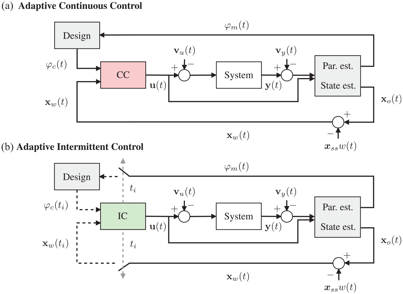
The continuous and intermittent controllers from Figure 1 can be extended to account for time-varying system parameters by adding an adaptation layer. In this work, this is achieved by using a self-tuning architecture^20,21 that runs a state and parameter estimation algorithm continuously, which tracks both, the evolving states and the system parameters, to then redesign the controller based on the updated parameter values. In the adaptive continuous controller, this redesign is executed at every iteration, whereas in the adaptive intermittent controller, this is done only once an event is detected, that is, at $t_i$ . These concepts are illustrated in Figure 2, where the block diagram of a general adaptive intermittent controller (Figure 2(b)) is presented alongside its continuous counterpart (Figure 2(a)). The online estimation problem implies the use of a recursive algorithm capable of tracking parameter changes in real-time using only the control input $\mathbf{u}(t)$ and the system output $\mathbf{y}(t)$ . This can be done using techniques such as recursive least squares; ²¹ however, the controllers introduced in this article exploit the flexibility of joint Kalman filters ²⁶ to estimate not only system parameters but also the states, in one single routine. We will start by establishing the main aspects of the redesign stage for both controllers, to then focus on the estimation algorithms.

Figure 2.

Continuous and intermittent adaptive control: (a) The Par est./State est. block is in charge of generating the estimated state and ${\mathbf{x}}_o(t)$ the model parameters ${\phi }_m(t)$ continuously. The input $\mathbf{u}(t)$ and the output $\mathbf{y}(t)$ can be corrupted by input noise ${\mathbf{v}}_u(t)$ and measurement noise ${\mathbf{v}}_y(t)$ , respectively. The Design block corresponds to the redesign stage and outputs new parameters ${\phi }_c(t)$ to the standard CC from Figure 1. (b) The events from the standard IC are used not only to sample the states ${\mathbf{x}}_w(t)$ but also the estimated system parameters ${\phi }_m(t)$ at $t_i$ . This yields a set of redesigned controller values ${\phi }_c(t_i)$ . Grey blocks show the components that provide adaptation capabilities and the dashed lines are quantities defined only at $t_i$ .

Adaptive continuous control

The entries in matrices $\mathbf{A}$ , $\mathbf{B}$ , and $\mathbf{C}$ in equation (1), are linear expressions of the system parameters. If a parameter estimation routine is used to update specific entries in these matrices, then a controller redesign can take place. Assuming that these parameters are obtained in real-time by a recursive estimator, a new set of system matrices can be computed as follows

$$\mathbf{A}=\mathbf{A}({\phi }_m(t)),\mathbf{B}=\mathbf{B}({\phi }_m(t))$$

(18)

The vector ${\phi }_m(t)$ contains the selected system parameters to be estimated continuously. The re-computation of matrices $\mathbf{A}$ and $\mathbf{B}$ for the adaptive continuous controller takes place at every iteration; this operation can be considered as the initial step of the redesign process. Once the new system matrices are obtained, the quantities established in the underlying continuous design stage have to be recomputed. This involves solving the system in equation (5) to obtain ${\mathit{x}}_{\mathrm{ss}}$ and ${\mathit{u}}_{\mathrm{ss}}$ , followed by a new state-feeback gain $\mathbf{k}$ generated via the LQR approach and the computation of the predicted states ${\mathbf{x}}_p(t)$ using equation (4). The final control law that is applied to the system is given in equation (2).

Adaptive Intermittent Control

The basic approach of adaptive IC is the same as for continuous control, with the fundamental difference that adaptive IC has to go through the redesign cycle less often than adaptive CC, which is an advantage from a computational point of view: the set of system parameters ${\phi }_m$ is estimated continuously but is only used at event times, $t_i$ . Based on this, the estimated matrices $\mathbf{A}$ and $\mathbf{B}$ are defined as

$${\mathbf{A}}_i=\mathbf{A}({\phi }_m(t_i)),{\mathbf{B}}_i=\mathbf{B}({\phi }_m(t_i))$$

(19)

This means that ${\mathbf{A}}_i$ and ${\mathbf{B}}_i$ stay constant until the next event occurs at $t_{i+1}$ , that is, during the open-loop interval ${\Delta }_i^{\mathrm{ol}}$ . With the new system matrices defined at $t_i$ , the re-computation of the steady-state components and state-feedback gains can be performed giving ${\mathit{x}}_{\mathrm{ss}}(t_i)$ , ${\mathit{u}}_{\mathrm{ss}}(t_i)$ , and ${\mathbf{k}}_i=\mathbf{k}(t_i)$ , using the same methods as before.

Adaptive IC requires the definition of additional quantities that depend on the newly obtained ${\mathbf{k}}_i$ and the system matrices ${\mathbf{A}}_i$ and ${\mathbf{B}}_i$ . One of them is the hold mechanism, ${\mathbf{A}}_h$ , defined in equation (8), which dictates the behaviour during the open-loop interval ${\Delta }_i^{\mathrm{ol}}$ and is matched to the closed-loop matrix ${\mathbf{A}}_c$ when an event is generated, that is

$${\mathbf{A}}_h(t_i)={\mathbf{A}}_c(t_i)={\mathbf{A}}_i-{\mathbf{B}}_i{\mathbf{k}}_i$$

(20)

Expression (20) implies that ${\mathbf{A}}_h$ stays constant throughout the open-loop interval. To simplify notation, we will write ${\mathbf{A}}_{h_i}={\mathbf{A}}_h(t_i)$ to represent the hold at event times $t_i$ .

The aforementioned hold mechanism uses the predicted states ${\mathbf{x}}_p(t_i-t_d)$ at $t_i$ to reset its internal state as shown in equation (10). The operations involved in the calculation of ${\mathbf{x}}_p$ depend on the dynamical system defined in equation (12), which has a solution at $\tau =t_d$ given by equation (16). This solution relies on matrix ${\mathbf{A}}_{\mathrm{ph}}$ , which needs to be re-calculated when the parameters are updated at $t_i$

$${\mathbf{A}}_{\mathrm{ph}}(t_i)=\left[\begin{array}{cc}{\mathbf{A}}_i\hfill & -{\mathbf{B}}_i{\mathbf{k}}_i\hfill \\ \multicolumn{1}{c}{0_{n\times n}}& {\mathbf{A}}_{h_i}\hfill \end{array}\right]$$

(21)

Finally, an IC law is established as follows

$$\mathbf{u}(t)=-{\mathbf{k}}_i{\mathbf{x}}_h(\tau )+{\mathit{u}}_{\mathrm{ss}}(t_i)w(t)$$

(22)

where the hold states ${\mathbf{x}}_h(\tau )$ are reset according to equation (10) when there is a feedback event.

The stability of the proposed controllers is guaranteed by the underlying continuous design methodology that serves as a basis for IC, as it defines the closed-loop performance and the characteristics of the response. In this work, the LQR approach ²⁵ was used to obtain values of the feedback gain $\mathbf{k}$ that result in stable closed-loop behaviour (see equation (9)). Other design approaches could also be used such as directly assigning the location of the closed-loop poles via pole-placement methods. A more detailed treatment of the stability properties of the system-matched hold version of IC is given in Gawthrop and colleagues.^4,23

The general IC framework can be designed in such a way that constant disturbances affecting the system are accounted for, for example, by including a disturbance observer as a part of the state estimation process.^2,4 In order to simplify the analysis for this article, no external disturbances were added to the simulations or to the real-time experiments, and a disturbance observer has not been included in the system.

State and parameter estimation

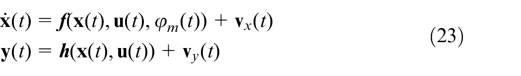
As discussed above, the general structure of the Kalman filter allows it to be implemented as a joint estimator, which tracks both system states and parameters in a single algorithm. ²⁶ Let us assume the following model for the system

$$\begin{array}{c}\multicolumn{1}{c}{\stackrel{·}{\mathbf{x}}(t)=\mathit{f}(\mathbf{x}(t),\mathbf{u}(t),{\phi }_m(t))+{\mathbf{v}}_x(t)}\\ \multicolumn{1}{c}{\mathbf{y}(t)=\mathit{h}(\mathbf{x}(t),\mathbf{u}(t))+{\mathbf{v}}_y(t)}\end{array}$$

(23)

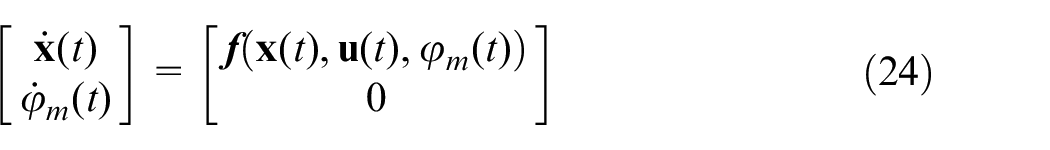
The process and measurement noise vectors, ${\mathbf{v}}_x\in {\mathbb{R}}^n$ and ${\mathbf{v}}_y\in {\mathbb{R}}^{n_y}$ respectively, are considered Gaussian with zero mean, with covariance matrices $\mathbf{Q}$ and $\mathbf{R}$ that are known. In a Joint estimation process, the state vector $\mathbf{x}(t)$ is augmented with the selected system parameters as additional states, making the assumption that they do not change through time. If the augmented state vector is defined as ${\mathbf{x}}_{\mathrm{aug}}(t)={[\mathbf{x}(t){\phi }_m(t)]}^T$ , then the updated model can be written as follows

$$\left[\begin{array}{c}\stackrel{·}{\mathbf{x}}(t)\hfill \\ \multicolumn{1}{c}{{\stackrel{·}{\phi }}_m(t)}\end{array}\right]=\left[\begin{array}{c}\mathit{f}(\mathbf{x}(t),\mathbf{u}(t),{\phi }_m(t))\hfill \\ \multicolumn{1}{c}{0}\end{array}\right]$$

(24)

The Kalman filter formulation is then applied to the model defined in equation (24). In this work, a nonlinear version of the filter known as the unscented Kalman filter (UKF) ²⁷ is implemented, where statistical transformations are used to avoid the linearisation process involved in linear formulations of the filter, such as the extended Kalman filter (EKF). ²⁸ The implementation details of the UKF are given in Appendix 1.

Augmented rotational pendulum model for parameter estimation

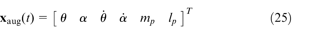
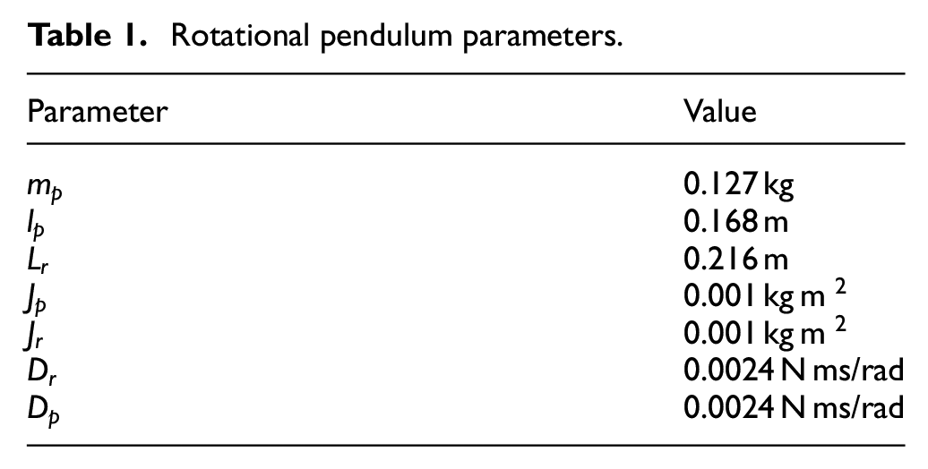
A rotational pendulum model was selected to illustrate the concepts introduced in the previous section. This system is well known in the control literature and poses interesting challenges from a control perspective. The model describes the dynamics of a physical rotational pendulum based on the SRV-02 and ROTPEN-E modules from Quanser (Canada). The details of the model, including the nonlinear and linear equations describing it, are shown in Appendix 2. The nominal values for all the parameters in the model are shown in Table 1. To design the adaptive controllers for the rotational pendulum, first the augmented model that adds the system parameters as extra states to the original state-vector needs to be derived. These system parameters will be estimated in order to update the corresponding controller in the redesign stage. For this system, the state-vector is defined in equation (47), which needs to be augmented by the system parameters to obtain the form given by equation (24). The arm and pendulum angles are the outputs of the system and can be defined in vector form as $\mathbf{y}(t)=[\theta \alpha {]}^T$ . Considering the case where the mass of the pendulum $m_p$ and the length $l_p$ are time-varying parameters, ${\phi }_m(t)=[m_p{l}_p{]}^T$ , then the augmented state vector upon which the UKF is designed can be written as

$${\mathbf{x}}_{\mathrm{aug}}(t)={\left[\theta \alpha \stackrel{·}{\theta }\stackrel{·}{\alpha }{m}_p{l}_p\right]}^T$$

(25)

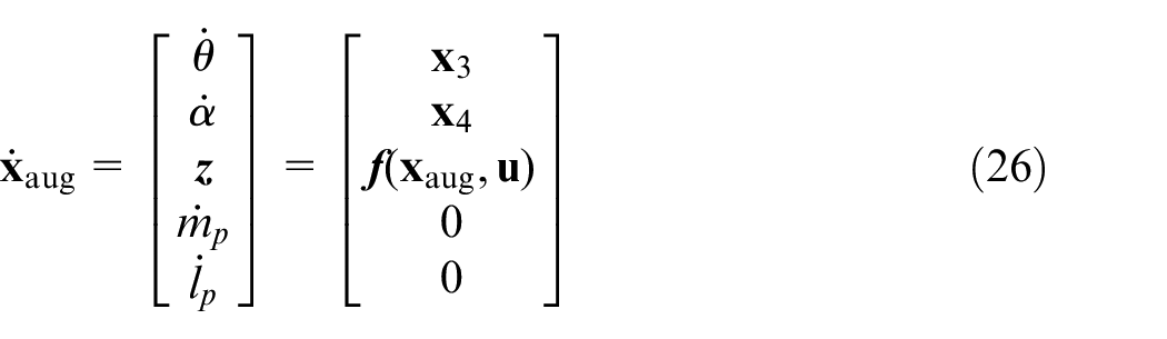
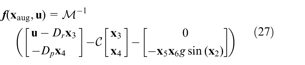
where $\theta$ and $\alpha$ are the arm and pendulum angles, respectively. By dropping time dependency notation for simplicity, establishing $\theta ={\mathbf{x}}_1$ , $\alpha ={\mathbf{x}}_2$ , $\stackrel{·}{\theta }={\mathbf{x}}_3$ , $\stackrel{·}{\alpha }={\mathbf{x}}_4$ , $m_p={\mathbf{x}}_5$ , and $l_p={\mathbf{x}}_6$ , and with the help of equation (25), it is possible to write

$${\stackrel{·}{\mathbf{x}}}_{\mathrm{aug}}=\left[\begin{array}{c}\stackrel{·}{\theta }\hfill \\ \multicolumn{1}{c}{\stackrel{·}{\alpha }}\\ \multicolumn{1}{c}{\mathit{z}}\\ \multicolumn{1}{c}{{\stackrel{·}{m}}_p}\\ \multicolumn{1}{c}{{\stackrel{·}{l}}_p}\end{array}\right]=\left[\begin{array}{c}{\mathbf{x}}_3\hfill \\ \multicolumn{1}{c}{{\mathbf{x}}_4}\\ \multicolumn{1}{c}{\mathit{f}({\mathbf{x}}_{\mathrm{aug}},\mathbf{u})}\\ \multicolumn{1}{c}{0}\\ \multicolumn{1}{c}{0}\end{array}\right]$$

(26)

where $\mathit{z}=[\stackrel{··}{\theta }\stackrel{··}{\alpha }{]}^T$ and $\mathit{f}(·)$ being

$$\begin{array}{c}\multicolumn{1}{c}{\mathit{f}({\mathbf{x}}_{\mathrm{aug}},\mathbf{u})={\mathcal{M}}^{-1}}\\ \multicolumn{1}{c}{(\left[\begin{array}{c}\mathbf{u}-D_r{\mathbf{x}}_3\hfill \\ \multicolumn{1}{c}{-D_p{\mathbf{x}}_4}\end{array}\right]-\mathcal{C}\left[\begin{array}{c}{\mathbf{x}}_3\hfill \\ \multicolumn{1}{c}{{\mathbf{x}}_4}\end{array}\right]-\left[\begin{array}{c}0\hfill \\ \multicolumn{1}{c}{-{\mathbf{x}}_5{\mathbf{x}}_{6}g\sin ({\mathbf{x}}_2)}\end{array}\right])}\end{array}$$

(27)

The function $\mathit{f}(·)$ corresponds to the solution in terms of the angular accelerations based on ${\mathbf{x}}_{\mathrm{aug}}$ and the torque $\mathbf{u}$ , which serves as the only control input in the system. The matrices $\mathcal{M}$ and $\mathcal{C}$ , as well as constants $D_r$ and $D_p$ , are defined in Appendix 2.

Table 1.

Rotational pendulum parameters.

Parameter	Value
$m_p$	0.127 kg
$l_p$	0.168 m
$L_r$	0.216 m
$J_p$	0.001 kg m ${}^2$
$J_r$	0.001 kg m ${}^2$
$D_r$	0.0024 N ms/rad
$D_p$	0.0024 N ms/rad

Controller design and UKF parameters

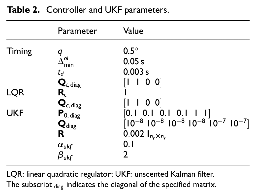
The controller and joint Kalman filter parameters that were used for the simulations are shown in Table 2. In the first section, the timing and threshold parameters are shown (applicable only to IC), followed by the LQR controller design matrices ${\mathbf{R}}_c$ and ${\mathbf{Q}}_c$ which are defined offline to determine the state-feedback gain $\mathbf{k}$ . ²⁵

Table 2.

Controller and UKF parameters.

	Parameter	Value
Timing	$q$	0.5°
	${\Delta }_{\min }^{\mathrm{ol}}$	0.05 s
	$t_d$	0.003 s
	${\mathbf{Q}}_{t,\mathrm{diag}}$	$[1100]$
LQR	${\mathbf{R}}_c$	$1$
	${\mathbf{Q}}_{c,\mathrm{diag}}$	$[1100]$
UKF	${\mathbf{P}}_{0,\mathrm{diag}}$	$[0.10.10.10.111]$
	${\mathbf{Q}}_{\mathrm{diag}}$	$[{10}^{-8}{10}^{-8}{10}^{-8}{10}^{-8}{10}^{-7}{10}^{-7}]$
	$\mathbf{R}$	$0.002{\mathbf{I}}_{n_y\times n_y}$
	${\alpha }_{\mathrm{ukf}}$	$0.1$
	${\beta }_{\mathrm{ukf}}$	$2$

LQR: linear quadratic regulator; UKF: unscented Kalman filter.

The subscript ${}_{\mathrm{diag}}$ indicates the diagonal of the specified matrix.

The UKF algorithm parameters (described in Appendix 1) that need to be initialised before execution are shown in the final section of Table 2, including the initial error matrix ${\mathbf{P}}_o$ , the process noise $\mathbf{Q}$ , and measurement noise $\mathbf{R}$ covariance matrices. The off-diagonal elements of all of them are 0. Both ${\mathbf{P}}_o$ and $\mathbf{Q}$ have a dimension of $6\times 6$ due to the UKF being applied to the augmented state-vector defined in equation (25). The values of the parameter that controls the spread of the sigma points involved in the unscented transformation, ${\alpha }_{\mathrm{ukf}}$ , and the a-priori state distribution, ${\beta }_{\mathrm{ukf}}$ , are shown for reference (Wan and Van Der Merwe). ²⁹

The time delay, $t_d$ , was set to a very small value (i.e. $0.003\mathrm{s}$ ), as the delays are thought to be negligible.

Simulation scenarios

In this section, simulations with time-varying system parameters are evaluated. Both adaptive CC and IC were implemented using the UKF as a combined state-parameter estimator, which was started from the following vector of initial conditions ${\mathbf{x}}_o(0)=[05.15000.40.5]$ , this assigns 5.15° to the pendulum angle $\theta$ and the values of 0.4 kg and 0.5 m to $m_p$ and $l_p$ , respectively. As shown in Figure 2, ${\mathbf{v}}_u\in {\mathbb{R}}^{n_u}$ and ${\mathbf{v}}_y\in {\mathbb{R}}^{n_y}$ correspond to the input and measurement noise vectors, respectively; since, there are two outputs in the system $(n_y=2)$ , then ${\mathbf{v}}_y$ is also a two-dimensional vector. These signals were defined as randomly seeded Gaussian noise with $|{\mathbf{v}}_u|=0.01$ and $|{\mathbf{v}}_y|=0.001$ as the respective amplitudes.

Simulation results

Continuous vs Intermittent Control

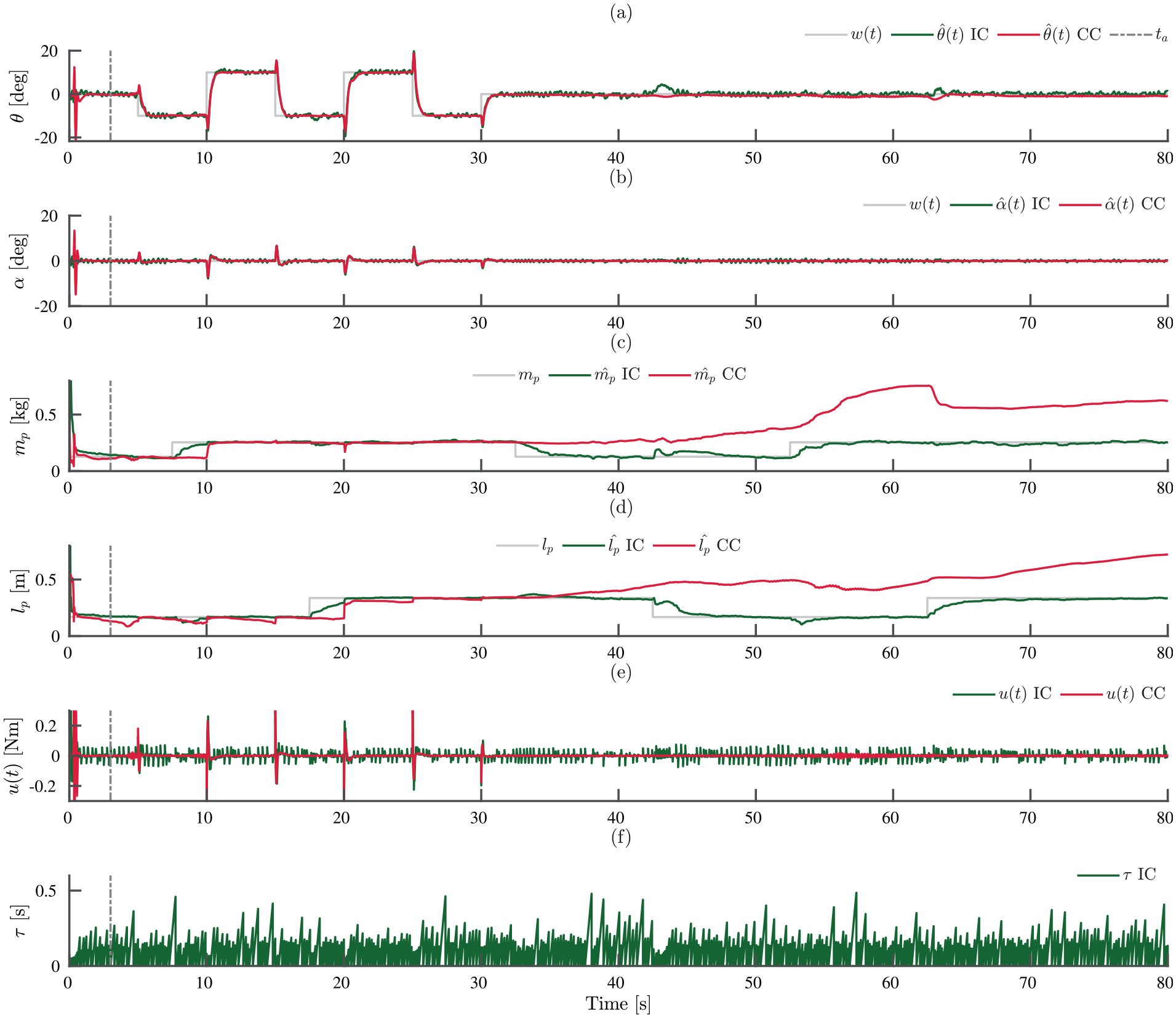
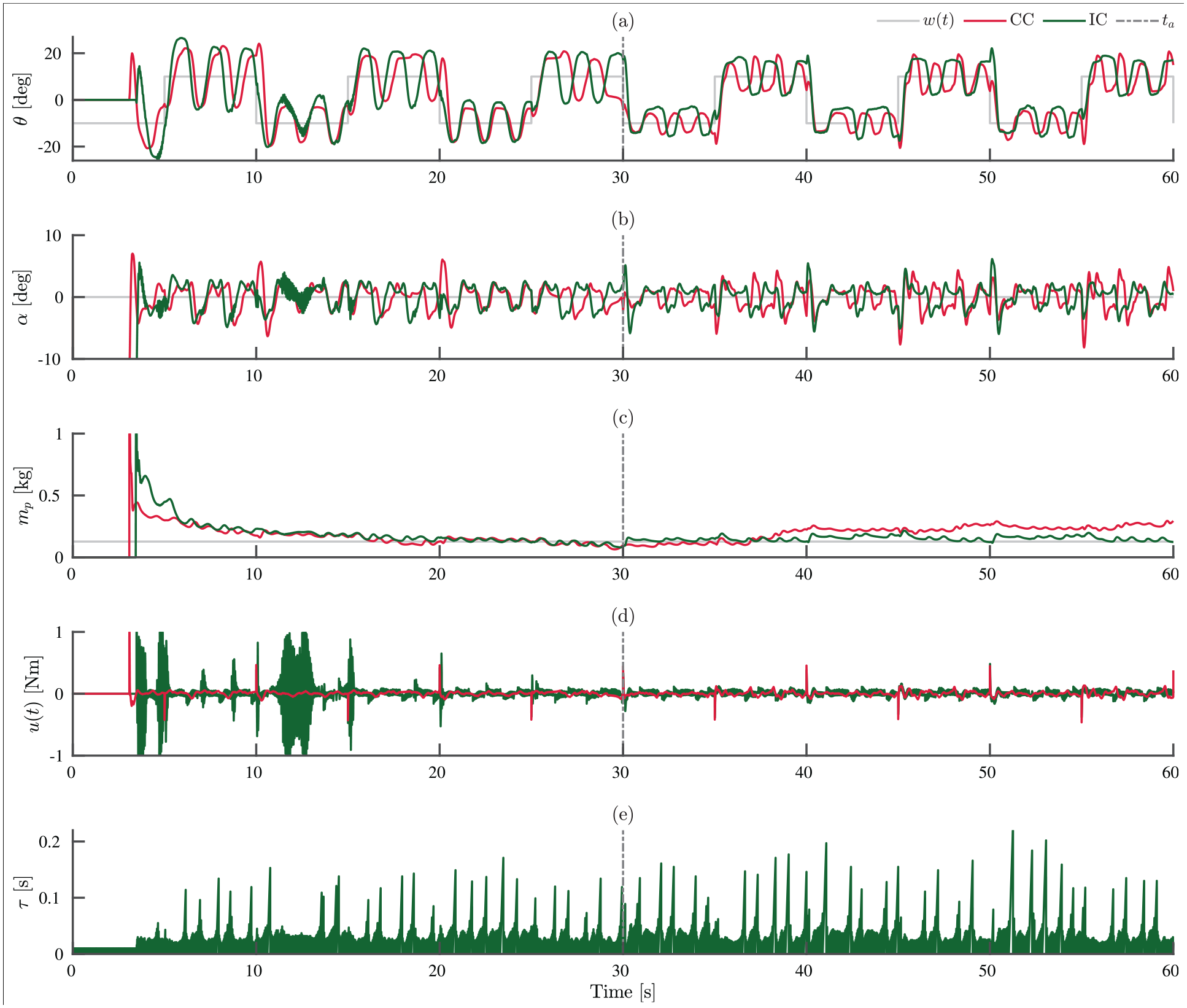
In the first simulation, the pendulum arm angle $\theta$ follows the reference $w(t)$ , which initially switches between 10° and −10° with a period of 10 s, while keeping the pendulum angle $\alpha$ as close as possible to 0°. After 30 s, the reference for $\theta$ becomes 0, cf. Figure 3(a, b). The pendulum length, $l_p$ , and its mass, $m_p$ , are varied during the simulation, which effectively changes the dynamics of the plant at different times. The nominal value of $m_p$ is 0.127 kg, which is used to start the simulation. At $t=7.5\mathrm{s}$ , it is increased by a factor of 2. The nominal starting length is $l_p=0.168\mathrm{m}$ , which is increased by a factor of 2 at $t=17.5\mathrm{s}$ . After 32.5 s, $m_p$ is returned to its nominal value while $l_p$ returns to its starting value at 42.5 s. Finally, these two parameters are doubled once again at 52.5 and 62.5 s, respectively (cf. Figure 3(c) and (d)).

Figure 3.

Responses for the simulation study using adaptive version of CC and IC: (a) estimated arm angle $\hat{\theta }$ , (b) estimated pendulum angle $\hat{\alpha }$ , (c) estimated pendulum mass ${\hat{m}}_p$ , (d) estimated pendulum length ${\hat{l}}_p$ , (e) control input $\mathbf{u}(t)$ , and (f) behaviour of the intermittent time $\tau$ (which only applies to IC). The time when adaptation is enabled, $t_a$ is represented by a grey vertical line at 3 s. The reference $w(t)$ is shown in grey for both angles. The trajectories of all these variables are shown in red for CC and in green for IC.

The results of the simulations are shown in Figure 3, where the estimated angles $\hat{\theta }$ and $\hat{\alpha }$ are shown in (a) and (b), the estimated parameters ${\hat{m}}_p$ and ${\hat{l}}_p$ in (c) and (d), and the control input $\mathbf{u}(t)$ as well as $\tau$ (which applies to IC only) in (e) and (f). The results in red correspond to CC and the ones in green are for IC. The controllers started using the estimated parameters at $t_a=3\mathrm{s}$ , shown by a grey vertical line. From Figure 3(a) and (b), we can see that both angles follow closely the corresponding reference. During the initial part of the simulation, where the system is excited due to periodic changes in the arm angle reference, both CC and IC estimate the updated values of $m_p$ and $l_p$ well (Figure 3(c) and (d)); however, IC does this faster than CC, continuously, without depending on the excitation due to the change in reference angle (between 5 and 10 s for $m_p$ and between 15 and 20 s for $l_p$ ). In contrast, CC only adjusts to the correct parameter value when the reference $w(t)$ changes at $t=10\mathrm{s}$ and $t=20\mathrm{s}$ .

Interestingly, when the reference $w(t)$ switches from a tracking regime to a regulation case (after $t=30\mathrm{s}$ ), the parameter estimates for IC in Figure 3(c) and (d) converge to their expected values, whereas CC is not capable of estimating the parameters correctly with the estimation error growing after $t=50\mathrm{s}$ . This is likely due to a lack of excitation in the CC control signal $\mathbf{u}(t)$ (cf. Figure 3e). On the contrary, IC generates a control signal that is higher in amplitude, compared to CC, ensuring persistent excitation which benefits the parameter estimation process.

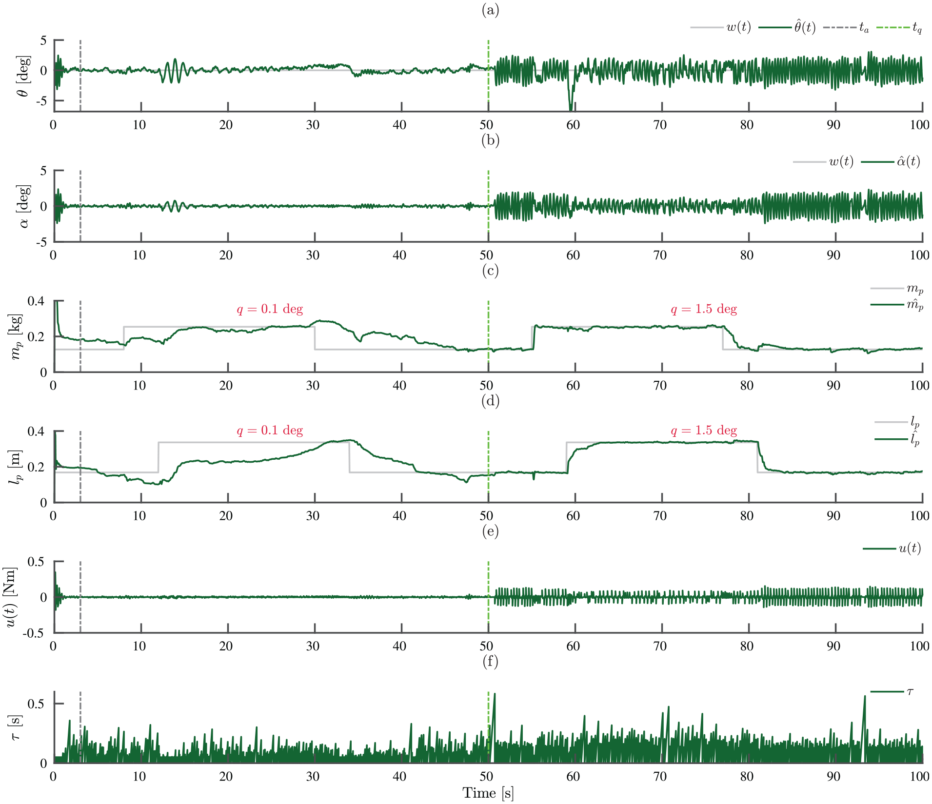
The effect of the event threshold

The event threshold $q$ has a critical role in IC, defining how sensitive the system will be to errors and therefore establishing if feedback is used more or less often. In the context of parameter adaptation, the threshold has the added benefit of acting as variable that we can manipulate to control how much the system is excited, which affects the parameter estimation rate of adaptive IC. To demonstrate this effect, we evaluated the adaptive IC in a regulation case ( $w(t)=0$ for both angles). Two sets of parameter changes for $m_p$ and $l_p$ were established, the first is applied between 0 and 50 s, followed by a second change between 50 and 100 s. Both of these changes were equal in terms of amplitude, doubling the nominal value of the parameter when the change was applied. During each of these time intervals, a different value of the threshold $q$ was used, starting with 0.1° (i.e. less than in the previous simulation) and switching to a threshold of 1.5° (i.e. larger than previously). All other simulation parameters remain unchanged (cf. Tables 1 and 2).

The results of this simulation are shown in Figure 4 which displays the same quantities as in Figure 3. The moment in time when the value of the threshold changes is indicated by a green dashed vertical line at 50 s, denoted as $t_q$ . The estimated parameters ${\hat{m}}_p$ and ${\hat{l}}_p$ , shown in Figure 4(c) and (d), exhibit different estimation rates directly after their true values change. For a threshold of 0.1° ( $t<50\mathrm{s}$ ), the estimated parameters slowly converge to the true values. Once the second threshold of 1.5° is enforced at $t_q$ , the estimates converge at a significantly faster rate, that is, almost instantly for ${\hat{m}}_p$ and in around 3–4 s for ${\hat{l}}_p$ .

Figure 4.

Responses for the simulation study, using adaptive IC, when the thresholds are varied throughout the simulation:(a) estimated arm angle $\hat{\theta }$ , (b) estimated pendulum angle $\hat{\alpha }$ , (c) estimated pendulum mass ${\hat{m}}_p$ , (d) estimated pendulum length ${\hat{l}}_p$ ,(e) control input $\mathbf{u}(t)$ , and (f) behaviour of the intermittent time $\tau$ . The time when adaptation is enabled, $t_a$ is represented by a grey vertical line at 3 s. The reference $w(t)$ is 0° for both the arm and pendulum angles. The threshold $q$ takes a value of 0.1° from 0 to 50 s, and after 50 s, its value is set to 1.5°. The time when the threshold changed is indicated with a green dashed vertical line and labelled as $t_q$ .

These different parameter estimation rates can be explained by the effect of the threshold $q$ on the system excitation through the control input $\mathbf{u}(t)$ , which is visible in the estimated angles $\hat{\theta }$ and $\hat{\alpha }$ (cf. Figure 4(a), (b) and (e)). Increasing the threshold value results in larger variations in the output, associated with a larger control input amplitude.

Real-time experiment

An experiment was performed using a real-time platform that includes a servo motor (SRV-02) that provides a torque to a rotating arm (ROTPEN-E), both modules are made by Quanser, see also Appendix 2, Figure 6. The two outputs (angles of the arm, $\theta$ and pendulum, $\alpha$ ) were measured by two incremental optical encoders and collected for processing with a National Instruments acquisition card (PCI-6024E). The arm angle $\theta$ was regulated via the voltage that the DC motor in the SRV-02 module produces. All controllers were implemented in MATLAB (Mathworks Inc.) using the Real-Time Windows target toolbox and zero-order hold approximations with a 1-ms sample interval. The values of threshold $q$ , the delay $t_d$ , and the minimum open-loop interval ${\Delta }_{\min }^{\mathrm{ol}}$ , that were used in the experiment were unchanged from the simulations and are defined in Table 2.

Both CC and IC were used to stabilise the pendulum angle $\alpha$ , and a periodic square signal $w(t)$ was used as a reference for the arm angle $\theta$ , ranging from −10° to 10°. In this experiment, only the pendulum mass $m_p$ was estimated as a system parameter; as a consequence, the last element of ${\mathbf{x}}_{\mathrm{aug}}$ in expressions (25) and (26), which corresponds to the length parameter $l_p$ , is removed. The total duration was 60 s, starting with 30 s of evolution based on a design that used a pendulum mass value of $m_p=0.07\mathrm{kg}$ , which is different compared to the nominal value in Table 1. At $t_a=30\mathrm{s}$ , the controllers were allowed to use the estimated parameters for redesign purposes, and this feature remained active until the end of the experiment.

Results

Figure 5 shows the outputs $\theta$ in Figure 5(a) and $\alpha$ in Figure 5(b), the estimated parameter ${\hat{m}}_p$ in Figure 5(c), as well as the control input $\mathbf{u}(t)$ in Figure 5(d) and the open-loop time $\tau$ in Figure 5(e). While oscillations around the reference $w(t)$ for $\theta$ can be observed throughout the experiment, these decrease after the redesigns take place at $t_a=30\mathrm{s}$ . In terms of amplitude, the oscillations are similar for CC and IC. The pendulum angle $\alpha$ , in Figure 5(b), also shows a slight reduction in amplitude when adaptation is enabled.

Figure 5.

Summary of the responses for the real-time experiment using adaptive CC and IC: (a) arm angle $\theta$ , (b) pendulum angle $\alpha$ , (c) estimated parameter $m_p$ , (d) control input $\mathbf{u}(t)$ , and (e) behaviour of the intermittent time $\tau$ . Each controller is shown in a different colour: red for CC and green for IC. For the first half of the experiment, the estimated mass values are not used, that is, both controllers use an erroneous mass of $m_p=0.07\mathrm{kg}$ . The time when adaptation is enabled, $t_a$ , is represented by a vertical line. The reference $w(t)$ is a square function for $\theta$ and 0° for $\alpha$ .

The parameter estimates (shown in Figure 5(c)) for CC start deviating from the true value after $t_a$ ; while the IC estimates stay close to $m_p$ for the entire duration of the experiment. The values of $\tau$ in Figure 5(e) (which only apply to IC, since CC does not have open-loop instances), increase slightly after the redesign starts at $t_a$ . During the experiment, $\tau$ reaches values between 0.1 and 0.2 s consistently, which is approximately 2–4 times greater than the imposed minimum open-loop interval ${\Delta }_{\min }^{\mathrm{ol}}=0.05\mathrm{s}$ . The control input in Figure 5(d) shows clearly the effect of the parameter mismatch (before $t_a$ ), where high control values are produced early in the experiment, these being higher for IC. When adaptation is enabled, the amplitude of the inputs reduces significantly because the estimates of $m_p$ , which are closer to the nominal value, are used to improve the controllers.

Comparing the results shown in Figure 5 with those of the simulation studies in Figure 3 and 4, it can be observed that the arm and pendulum angles for both IC and CC exhibit significantly larger oscillations in the case of the real-time system when compared to the simulated model. This is a result of un-modelled dynamics of the physical system, such as friction and gear backlash. Similarly, the open-loop periods $(\tau )$ in Figure 5, show a different pattern compared to the ones observed in simulation, as a result of the induced oscillations. Both $\theta$ and $\alpha$ follow their respective references; however, since the oscillations push these angles out of the no-triggering region imposed by the threshold $q$ , the open-loop intervals in $\tau$ exhibit a quasi-periodic cycle of slow and fast triggering (corresponding to low and high values of $\tau$ ).

Conclusion

The results of this article show the feasibility of adaptive intermittent controllers based on state and parameter estimation using joint Kalman filters. In our Kalman filter framework, an extended state-vector is used which is augmented with time-varying system parameters as additional states which are to be estimated. The estimated parameters are then used in a redesign stage to update the controller, leading to a self-tuning architecture. The adaptive intermittent controller was compared in simulations with an equivalent adaptive continuous controller. The adaptive intermittent controller was further evaluated on a real-time experimental control scenario. The results demonstrate how these adaptive controllers are useful in cases where the parameters of a system have a time-varying nature or when the model parameters assumed for control design do not approximate reality. The following list includes important remarks about IC and CC in an adaptation environment:

1. The use of IC results in persistent excitation of the system, which ensures that parameter changes are detected almost immediately and that they are tracked even if the system is not otherwise excited by a change in reference (cf. Figure 3). In contrast, CC requires external excitation (through a change in reference) to detect parameter changes. In the real-time experiment (cf. Figure 5), the pendulum mass estimate drifts away slowly from its true value due to missing excitation when CC is used.

2. The threshold $q$ can be used to adjust the degree of adaptation (i.e. the sensitivity to parameter changes). Smaller thresholds generate less excitation and consequentially slower adaptation (cf. Figure 4).

3. In adaptive IC, the controller redesign only happens at event times $t_i$ , which provides a computational advantage compared to CC where the redesign is done every iteration.

The adaptive IC introduced in this article relies on the concept of combining feedback and open-loop control. Opening the feedback loop as a mechanism to discover the causal links relating state variables and inputs has been mentioned before,^18,30 an idea that results from the observation that when a system operates under the influence of continuous feedback control, it becomes more difficult to clearly understand the effect of external components affecting the system such as noise or disturbances, as well as system parameters that change through time. On the contrary, small instances of open-loop control would result in rapidly growing errors, which reveals the causes that lead to them and clarifies the subsequent correcting actions.

A list of the main contributions of this article, which revolve around the aforementioned ideas, is provided in the interest of clarity:

• Adaptive IC is introduced as a framework that provides an acceptable steady-state response through a control signal that also generates enough excitation to detect system changes. This ability can be understood in terms of the stability–plasticity dilemma, ³¹ which raises the question of how a control methodology can be designed with the goal of remaining plastic in the presence of changes or uncertainty, while maintaining stability performance levels that have been achieved in part from past experience.

• Special emphasis is placed on the threshold parameter $q$ . In the adaptation context, this parameter not only determines when the events are generated, but it also sets the rate of adaptation by regulating how much error is allowed in the specified outputs, that is, how much the system can be excited. In practice, this becomes relevant since a closed-loop system could potentially be designed with this principle in mind: use a small threshold when precision control is needed, uncertainty is low, and where the main goal is to reduce variability; conversely, use large thresholds if the goal is to detect parametric changes in the system and redefine the control parameters to compensate accordingly.

A natural limitation of the proposed adaptive intermittent controller is that if due to design constraints, the outputs of a particular closed-loop process must have very small steady-state error levels, then the ability of using the threshold to regulate the adaptation rate could potentially be limited.