
Abstract
This study proposes an optimized hybrid visual servoing approach to overcome the imperfections of classical two-dimensional, three-dimensional and hybrid visual servoing methods. These imperfections are mostly convergence issues, non-optimized trajectories, expensive calculations and singularities. The proposed method provides more efficient optimized trajectories with shorter camera path for the robot than image-based and classical hybrid visual servoing methods. Moreover, it is less likely to lose the object from the camera field of view, and it is more robust to camera calibration than the classical position-based and hybrid visual servoing methods. The drawbacks in two-dimensional visual servoing are mostly related to the camera retreat and rotational motions. To tackle these drawbacks, rotations and translations in Z-axis have been separately controlled from three-dimensional estimation of the visual features. The pseudo-inverse of the proposed interaction matrix is approximated by a neuro-fuzzy neural network called local linear model tree. Using local linear model tree, the controller avoids the singularities and ill-conditioning of the proposed interaction matrix and makes it robust to image noises and camera parameters. The proposed method has been compared with classical image-based, position-based and hybrid visual servoing methods, both in simulation and in the real world using a 7-degree-of-freedom arm robot.
Keywords
Introduction
In order to modify the behaviour of robots in dealing with unstructured environments, vision sensors are commonly used to provide contact-less information about the environment. 1 Real-time information from the camera image provides feedback to control the motion of a robot. This approach is called visual servoing (VS) which is an effective method for handling uncertainties in an unknown environment.
VS contributes to modify the system to compensate deficiencies of a mechanism and to relax the mechanical inaccuracy and stiffness of the robot. 2 This ability comes from the fact that the feature errors are regulated directly in the task space. 3 Despite this fact, how to use the image information to control the motion of a robot always been a major challenge in robotics. VS adds complexities in image space, joint space and the intersection between these two (task space) which should be considered. 4 VS control approaches are broadly classified into three categories: image-based visual servoing (IBVS), position-based visual servoing (PBVS) and hybrid visual servoing (HVS).
IBVS method computes the feedback directly from extracted features in the image space. This method is more robust to the camera calibration and kinematic errors of the robot. 5 Furthermore, the image features are less likely to be lost from the image screen. 6 However, there exist drawbacks for IBVS; first, some controller’s commands are not physically executable as there is no direct control for Cartesian velocities of the robot’s end-effector (EE). 7 Second, an interaction matrix (image-Jacobian) is required to map velocities from image space to velocities in the workspace of the robot. Therefore, the poor conditioning of the Jacobian matrix could cause convergence problems such as singularities and local minima. 8 Consequently, PBVS was proposed to address the imperfections of IBVS. 9
In PBVS, feedback is computed using reconstructed Euclidean information to estimate the three-dimensional (3D) Cartesian pose of the target with respect to the camera pose. In PBVS method, interaction matrix problems (i.e. local minima and singularity) are avoided due to the direct calculation of the camera velocities from the task space errors; therefore, feasible trajectories for the robot could be generated. 10 However, any error in calibration of the camera could lead to an error in 3D estimation of the target, and subsequently, the entire tracking task. In addition, it is more possible to lose the features in the image screen, as the control feedback is generated from 3D estimation of the environment. 2
HVS was proposed to benefit from the advantages of IBVS and PBVS while avoiding the drawbacks of these two. 11 In HVS methods like switching, 2 1/2D and homography-based VS, the task function uses image space information combined with the Cartesian space. 12 However, hybrid methods come with some performance deficiencies that will be discussed in detail in section ‘Related works’.
Related works
Switching method is a type of HVS in which the controller switches between IBVS and PBVS with respect to (w.r.t.) their efficacy. 13 However, the controller suffers from discontinuities while switching occurs, especially when the object is close to the image borders. 14 Such discontinuities could be solved using sequencing methods; 15 nevertheless, the convergence time will increase. 2 Moreover, two failures in IBVS named camera retreat 8 and the Chaumette Conundrum could not be determined easily as image-Jacobian is not ill-conditioned in those configurations. 7 Therefore, switching between two methods (i.e. IBVS and PBVS) could not solve these kinds of complexities. 8 Even inducing rotational motions about the camera optic axis could not solve the Chaumette Conundrum, as rotational contributions cancel out one another.
Corke and Hutchinson 8 proposed a VS method that decouples the translation and rotation about Z-axis, from the image-Jacobian, in order to address the Chaumette Conundrum and the camera retreat. However, expensive computation of the pseudo-inverse is still challenging. Moreover, compensating the rotation errors about X-axis and Y-axis in the image-plane still produces unnecessary motion for the robot’s joints which are not preferable. 13
In 2 1/2D VS methods, the unnecessary motions are minimized by decomposing translations from the rotations. 16 But, these methods are computationally expensive too and require homography construction which is sensitive to image noise. 8 Another drawback of 2 1/2D VS method is its demand to have co-planar features for estimating the homography matrix. Otherwise, at least eight features are required for this estimation, while in other methods, four features are enough. 17 In addition, 2 1/2D VS decomposes homography to extract rotational parameters which come with non-unique solutions. 18
Recently, learning-based approaches (e.g. recurrent neural network (RNN), convolution neural network (CNN), reinforcement learning (RL) and extreme learning machine (ELM)) are widely used to tackle vision tracking problems which are difficult or computationally expensive to solve by classical control methods, such as singularity avoidance, local minima or complex computation of pseudo-inverse.19–21 Supervised learning approaches contribute to estimating the data output from previous experiences; therefore, the data set must be labelled in advance. However, unsupervised learning approaches find unknown patterns in a set of data. 22 Despite supervised learning approaches, it is not possible for regression applications to train the network without knowing the corresponding output values. 23 RNN has been used in Zhang and Li 24 to estimate the interaction matrix, but it requires a number of iterations to reduce the convergence speed. Hence, the network could not guarantee global optimization. Miljković et al. 21 proposed a controller that switches between neural RL and IBVS to solve the pseudo-inverse of the interaction matrix. However, huge chattering occurs in the computed camera velocities. Regression-based neural networks (NNs) have been considerably used to approximate the non-linear image-Jacobian.25–28 They suffer from local minima which are complex to avoid. 29 It is worth mentioning that using NN in approximating the hybrid interaction matrices is not widely investigated in the literature.
To tackle the above-mentioned problems, we proposed an optimized VS method called hybrid decoupled visual servoing (HDVS). The contributions of our proposed method in comparison with other classical VS methods have been illustrated in Figure 1. In the proposed method, all three rotations and translation in the Z-axis have been decoupled from the image-Jacobian. These four components’ errors will be regulated from the 3D reconstruction of the visual features. Consequently, the controller has independent control over translation in Z-axis and rotations. Thereafter, local linear model tree (LoLiMoT) NN has been used to approximate the pseudo-inverse of the proposed interaction matrix. Using LoLiMoT avoids singularities that could be happened in the interaction matrix, and reduces the computational complexities effectively. Accordingly, the controller becomes robust to the camera calibration errors and the image noises. LoLiMoT is a fast, effective neuro-fuzzy NN that learns a huge number of non-linear models. 30 LoLiMoT method guarantees global optimization solution which implies the generalization ability of the method. 30 Regression approaches are blind in detection of global minima, but LoLiMoT is axis orthogonal and operates by errors; thus, it will not stick in local minima. 31 The locality of this method provides online learning in one region without forgetting the other operating regions. 32 Not to mention that the number of required trial-and-error steps will be reduced in LoLiMoT approach. The proposed method is producing a more optimized trajectory, both in the image space and the joint space than other hybrid methods, in terms of control effort and the convergence time. In comparison with IBVS, HDVS generates more controllable trajectories for the robot during tracking the objects. Furthermore, it is less likely to lose the object from the camera field of view, in contrast to PBVS and HVS methods. The proposed HDVS method is robust to camera calibration and image noises. In the ensuing, the method will be discussed in detail and its efficacy will be validated in both simulation and the real world.
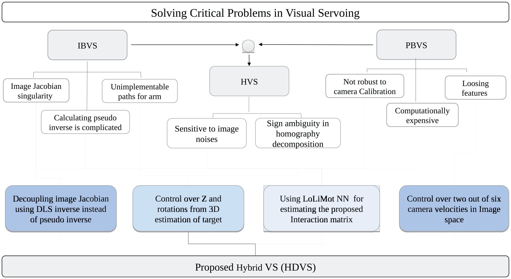
Problem domains in classical visual servoing and contributions of the proposed HDVS method.
Contributions of this study
Figure 1 depicts a framework for the proposed HDVS method, and it highlights the contributions of HDVS in comparison with other classical VS methods. The contribution of this study is summarized as follows:
HDVS generates more optimized Cartesian trajectories (better controllability) for the robot than IBVS and HVS. All three rotations and translation in the Z-axis have been decoupled from the image-Jacobian. The errors of these four components have been regulated from 3D reconstruction of the visual features. Since the remained components (translation in X-axis and Y-axis) are controlled directly in the image-plane, then a more optimized trajectory in the image-plane would be created than PBVS. Therefore, the object is less likely to be lost from the camera field of view. This contribution has been explained explicitly in section ‘Methodology’.
HDVS benefits from damped-least square (DLS) inverse instead of pseudo-inverse to generate the joint velocities. Therefore, HDVS reduces the effect of robot’s singularities and it assists to smooth the discontinuities created from decoupling process and adaptive gains. This contribution has been explained explicitly in section ‘Methodology’.
A set of LoLiMoT NNs has been trained in the presence of image noise to approximate the interaction matrix. Consequently, singularities of the interaction matrix would be avoided and computational complexities will be reduced effectively. Nevertheless, using LoLiMoT NN makes the controller robust to the camera calibration errors and image noises. This contribution has been explained explicitly in section ‘Methodology’.
The remainder of this study is as follows: in section ‘Methodology’, a brief review of different VS controllers will be presented. Then, our proposed method will be explained. In section ‘Simulation and experimental setup’, the simulation and experimental setup has been presented. Thereafter, in section ‘Results and discussion’, a comparison of different methods has been investigated followed by results. In section ‘Results and discussion’, our approach has been tested on the real robot while tracking a dynamic object. Eventually, in section ‘Conclusion’, a brief summary alongside the conclusion and the future ideas has been stated.
Methodology
The main goal of VS tasks is to regulate the error vector created by the visual features. In what follows, a brief background of well-known VS approaches is presented, followed by a detailed explanation of the proposed HDVS method.
IBVS
In IBVS, the controller feedback is directly attained by the features in the image space. An interaction matrix (image-Jacobian
This matrix for the
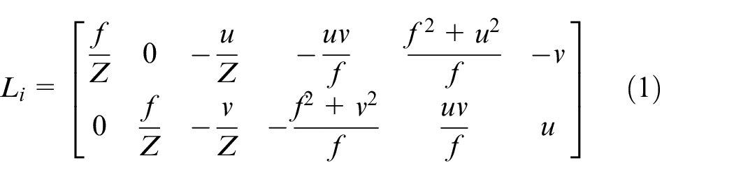
in which
where
PBVS
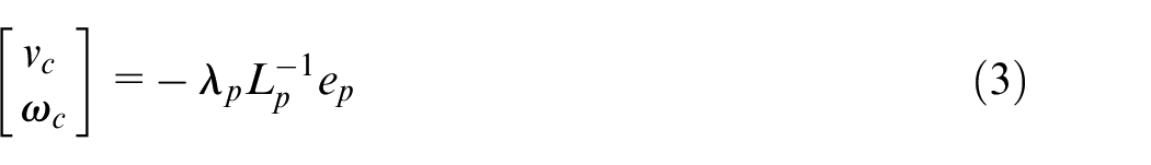
In PBVS, the feedback is obtained from the pose reconstruction of the environment. The pose estimation will be calculated with the help of Euclidean methods and camera parameters, from the camera image.
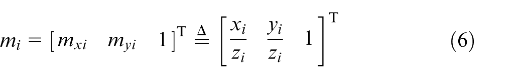
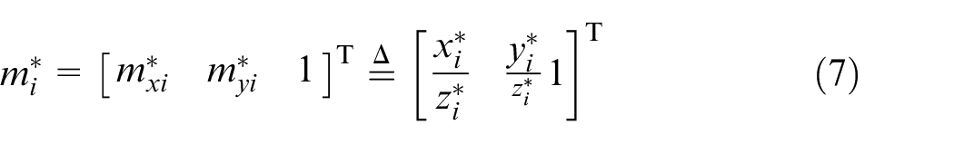
The Euclidean coordinate of the features in the camera frame is
where
where
where
Homography-based visual servoing
The homography-based visual servo control approaches mostly decompose the 6-degree-of-freedom (6-DOF) motion of the camera in two separate controllers in order to achieve the convergence goal: one for the translational components and the other one for the rotational components. Let
The error signal will be selected by the estimated position from the Euclidean information and directly from the image information 4
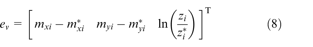

where


HDVS
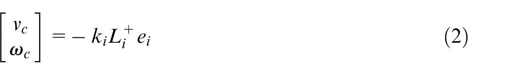
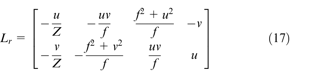
In the proposed method (HDVS), the translational velocity in Z-axis and three rotational velocities (the components that cause IBVS singularity and physically unimplemented motions for the robot) have been decoupled from the image-Jacobian matrix. The error of these four parameters will be calculated from 3D estimation of the target, while the translational velocities of the X and Y components will be calculated in two-dimensional (2D). The control law in the classical IBVS method is as follows

However, after decoupling the interaction matrix in HDVS, the control law will change to

where
Therefore
Since
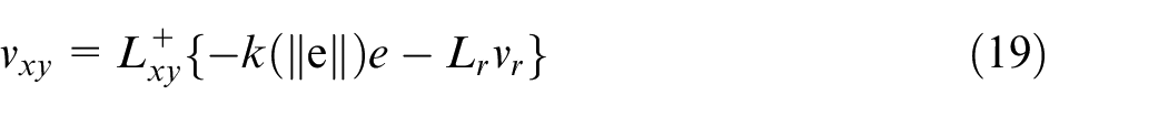
In order to decrease the convergence time, adaptive representation of the controller gain has been formulated as follows 34
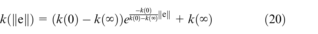
where

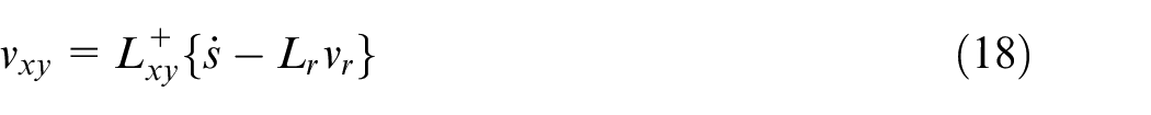
where

By solving equations (19) and (22) simultaneously, the camera velocity vector will be determined. The transformation matrix
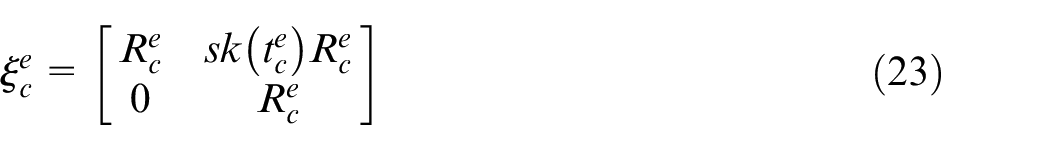
where
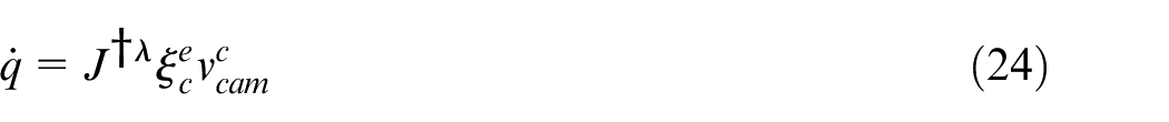
In this research, DLS inverse has been used instead of pseudo-inverse. Using DLS, the effect of robot’s singularities will be reduced and it will smooth the discontinuities created from decoupling process and using the adaptive gains. 36 It is worth mentioning that using regularization techniques could also help to reduce the effect of singularity configurations, but they will increase the convergence time. 37 DLS is formulated as follows 36
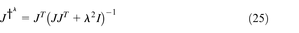
where
In Figure 2, the control schema of the proposed visual servoing controller is shown. Using a vision sensor mounted on the robot’s wrist, features will be detected and will be used as feedback of the controller. The red blocks represent image-based parts of the control loop, the blue blocks are position-based parts, and the grey blocks are the task space parts.
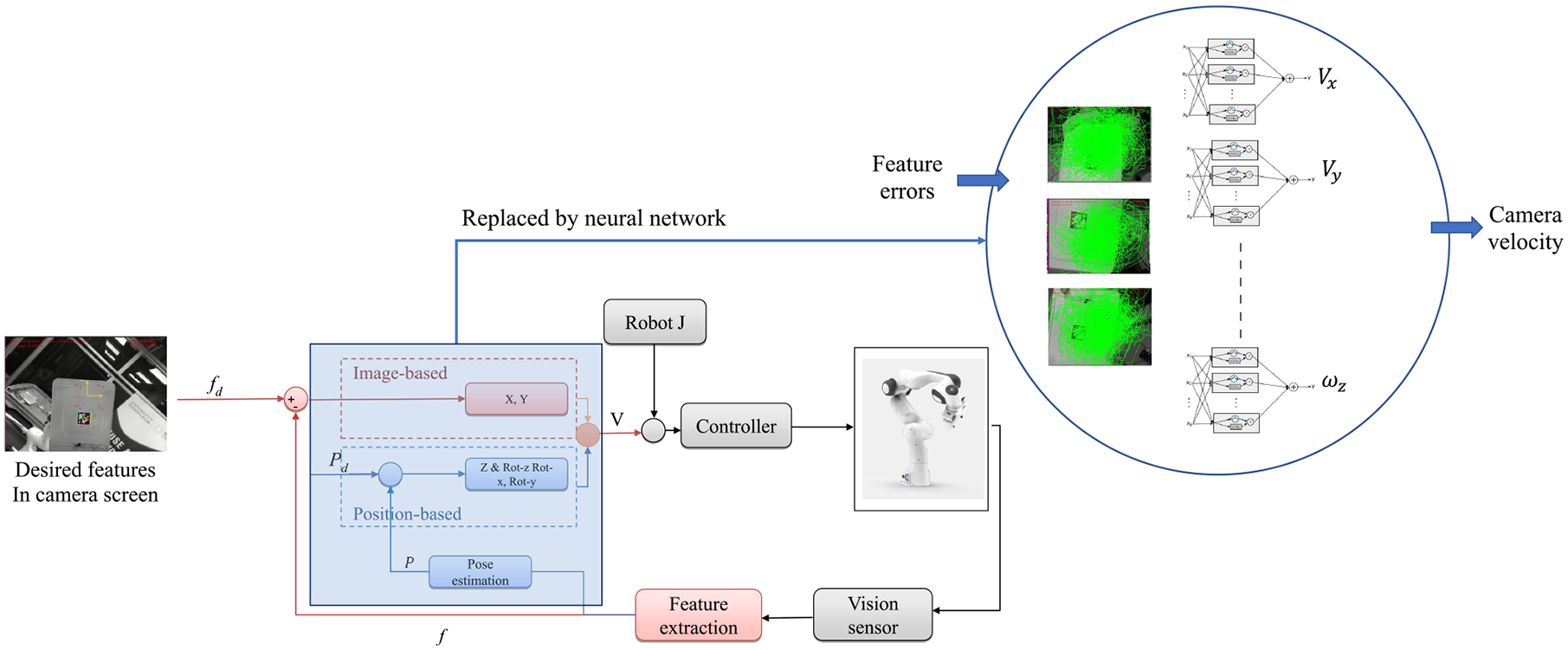
The control schema of the proposed visual servoing (HDVS) integrated with NN.
As it is depicted in the control block diagram (Figure 2), the camera velocities have been decoupled; two of them (translation in X and Y) have been considered in 2D (using pure features created from the image screen, as feedback). The remaining components have been considered in 3D (computed by partial 3D reconstruction of the environment attained by the extracted features). Thereafter, the computed velocities will be commanded to the robot. Using the robot’s Jacobian, the controller will exchange the desired camera velocities with the desired joint velocities. The computed joint velocities will be used as input of the robot velocity controller. As it was stated earlier, DLS inverse has been used instead of pseudo-inverse. Controlling the rotations and translation separately in the Z-axis is acquired from the 3D estimation of the visual features.
Estimation of camera velocities using NN
A trained NN is employed to provide an accurate estimation of the camera velocities from the feature errors (the interaction matrix role). The approximated equations by the NN are the combination of the right-hand side of equation (19) (including pseudo-inverse of
The LoLiMoT algorithm operates by the errors and it is axis orthogonal. Therefore, the network divides the space in a properly optimized way w.r.t. the errors. Other types of NNs, which work by the use of gradient descents, operate blind and cannot guarantee the global optimization. 39 The structure of the LoLiMoT network is depicted in Figure 3. A linear local model alongside a membership function is assigned to each neuron. For the allocated linear model, the validated area would be determined with an assigned membership function. The linear model is formulated as follows 40

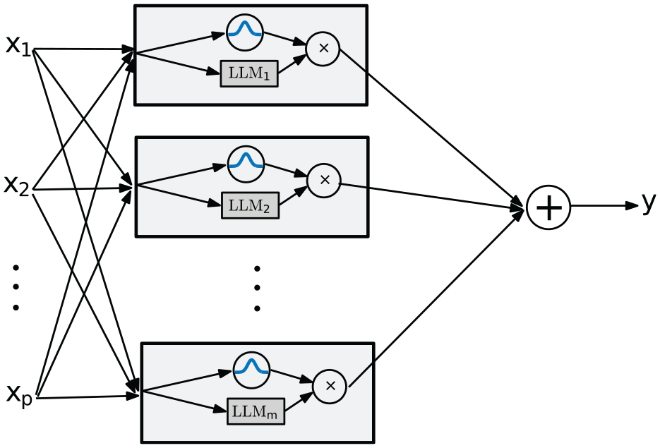
The structure of LoLiMoT NN with
In equation (26),
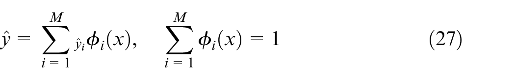
where
In equation (28),
Moreover, supplementary noise had been added to the NN input data set during training to improve its robustness to the image noises. The added Gaussian noise has a standard deviation of one and a mean of zero (white noise), generated by a pseudo-random number generator. Using NN, the complexity of 3D estimation of the target position and the pseudo-inverse of the decoupled image-Jacobian have been relaxed, as described in section ‘Methodology’.
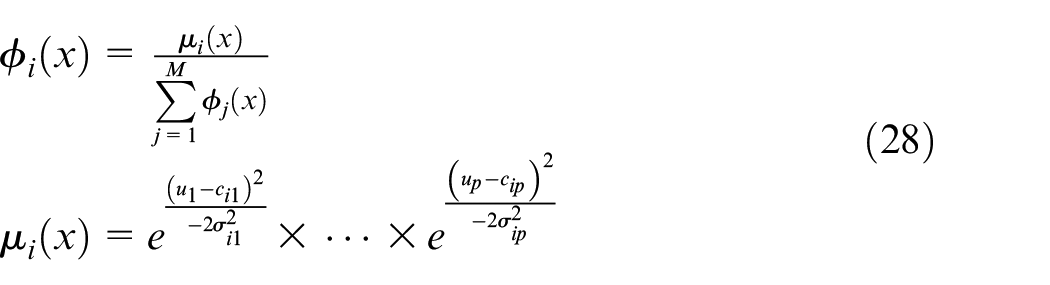
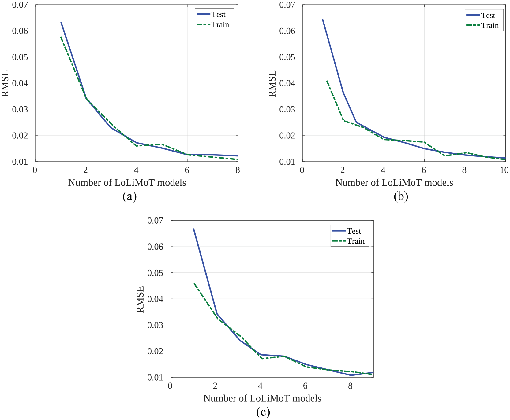
For each output, one LoLiMoT network has been used. Therefore, six NNs have been trained, which comes after six camera velocities. Each network has a different number of LoLiMoT models. The number of models achieved during learning process. The learning process stops when the test and train samples acquire a pre-defined accuracy. This accuracy will be checked by the root mean square of errors (RMSEs) in both test and train samples (RMSE of 0.01 m/s for translational velocities and RMSE of 0.01 rad/s for rotational velocities). Such a behaviour will effectively decrease the number of trial and errors.
The number of allocated LoLiMoT models (membership functions alongside linear local model) and RMSE of the trained NN for the test and the train samples have been depicted in Figures 4 and 5. Each LoLiMoT model consists of a linear local model alongside a Gaussian membership function.
RMSE of test and train samples of LoLiMoT neural network for translational camera velocity outputs: (a) RMSE of Vx, (b) RMSE of Vy and (c) RMSE of Vz.
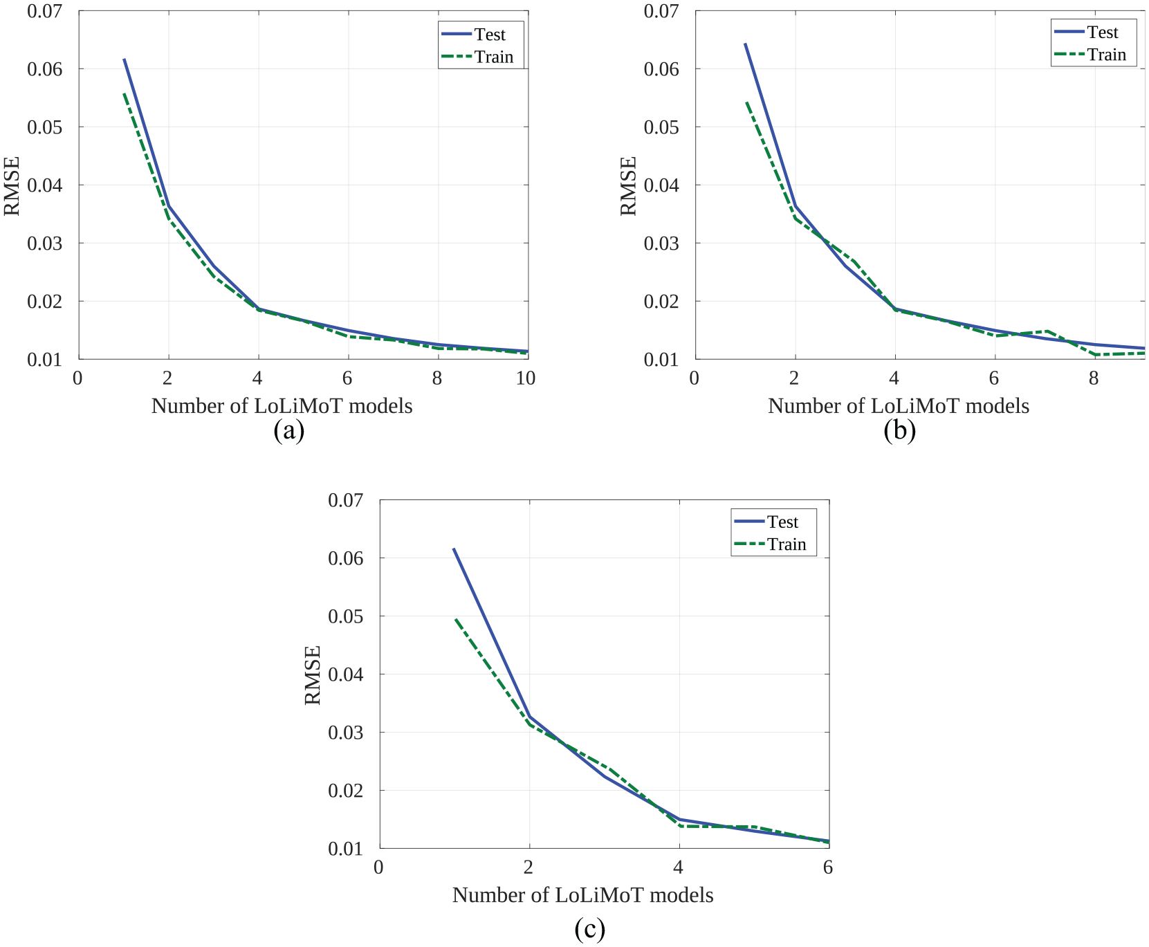
RMSE of test and train samples of LoLiMoT neural network for rotational camera velocity outputs: (a) RMSE of ωx, (b) RMSE of ωy and (c) RMSE of ωz.
As Figure 4(a) suggested, having 10 models is optimal in order to have the RMSE of 0.01 in test and train samples. Having more than 10 models is redundant and could lead the network to over-fitting. The number of LoLiMoT models is 9 for the prediction of velocity controller in Y direction (Figure 4(b)). These numbers are 6 for velocity in Z (Figure 4(c)).
In Figure 5(a), it can be seen that 8 LoLiMoT models are required for rotational velocity about X-axis, 10 models for rotational velocity about Y-axis (Figure 5(b)) and 9 LoLiMoT models for rotational velocity about Z-axis (Figure 5(c)). The trained set of these six networks will be used to predict the camera velocity required to perform the visual servoing task. The updated set of feature errors will be utilized for the networks at each iteration.
Simulation and experimental setup
In order to evaluate the efficacy of the method and to compare it with other techniques, the proposed method has been modelled in simulation using ROS/Gazebo. In Figure 6, a snapshot of the simulation environment in Gazebo is shown. Two Franka manipulators have been added to the simulation platform. One with a camera mounted on its wrist, for the VS purpose, and another one carrying a tag marker on a sheet attached to the EE.
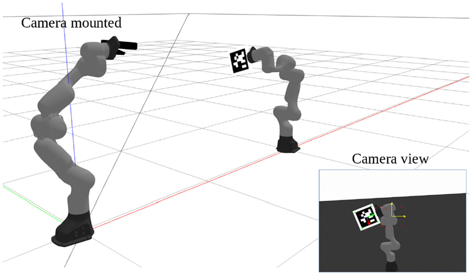
The simulation environment modelled in Gazebo.
The experimental setup is identical to the one used in the simulation. In this research, four corners of an AprilTag are used as points of interest. The Intel RealSense depth camera D435i has been used for eye-in-hand configuration as the vision sensor. For the VS operation, a system with the following processor had been used: AMD Ryzen 7 3700X 8-core processor 16 (thread) with 3.6 GHz base clock and 36 MB total cache. The experimental setup used in this research is depicted in Figure 7. In section ‘Results and discussion’, the behaviour of different control schemes in both simulation and experiments will be compared.
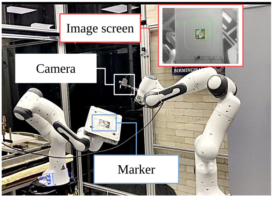
Experimental setup for visual servoing task.
Results and discussion
In order to evaluate the effectiveness of the HDVS method, various scenarios have been studied and compared with HVS, IBVS and PBVS approaches. To have a logical comparison, same adaptive gains have been used for every method
Case study 1: comparing the performance of PBVS with HDVS
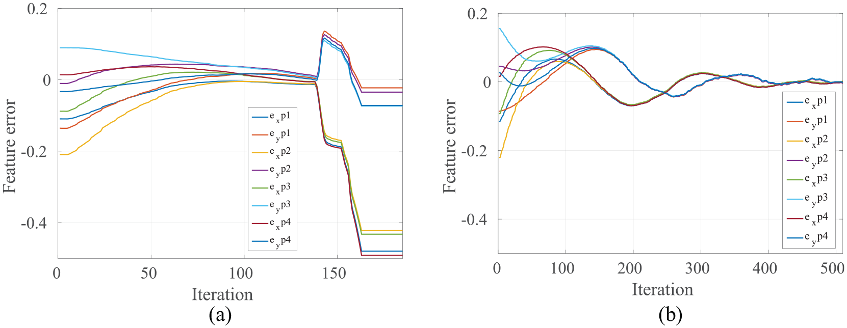
A case study has been defined to follow a pre-defined position of the target with an uncalibrated camera. The intrinsic calibration of the camera has been degraded by 20%. The performance of HDVS and PBVS in regulating the errors is illustrated in Figure 8. In Figure 8(a), it is shown that the position-based controller has been failed to track the features. It is depicted in Figure 8(a) that the controller could not follow the desired features from iteration 350. This failure comes from the fact that there is an error in the 3D estimation of the target generated by an uncalibrated camera.
Simulation result of tracking desired features with an uncalibrated camera for (a) PBVS and (b) HDVS.
The reason that PBVS is not robust to the camera calibration is that the errors in camera parameters propagated to the errors in 3D estimation of the target. However, HDVS is robust in terms of camera parameters. Figure 8(b) suggested that HDVS tracked the desired features successfully. This is because in HDVS camera, velocities are generated directly from the trained LoLiMoT NN. Collecting data for the NN has been done with accurate camera calibration. Therefore, it is not important how inaccurate is the camera calibration in online mode (i.e. robot during VS), the controller will work well and is highly robust to camera calibration errors.
Case study 2: comparing the performance of IBVS with HDVS
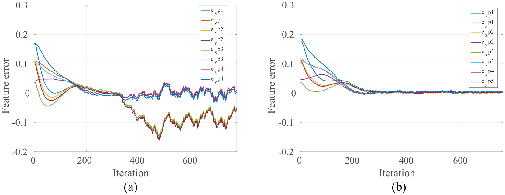
IBVS failures are mostly associated with the rotations about Z-axis (Chaumette Conundrum 7 ) and camera retreat. 8 Furthermore, camera ambiguities might happen between translations and rotations in the image-plane; this implies that different camera velocities could produce same motion of points in the image and some camera motions lead to no change in the image. 11 A case study has been defined in such that the desired features rotated 90° about the Z-axis. The performance of HDVS and IBVS in converging feature errors to zero is depicted in Figure 9.
Simulation results for (a) IBVS and (b) HDVS control approaches.
As shown in Figure 9, the controller will end up with an unpleasant behaviour in IBVS. Figure 9(a) shows that the errors could not converge to zero as the controller produces a large velocity in Z which makes the robot going to its joint limits. The main reason associates with this limitation is that reducing the rotation error about Z-axis in the image screen could be achieved by moving the camera away from the target (the so-called camera retreat phenomenon). Such a wrong decision in 2D could produce a large motion in the Z-axis in 3D. An extreme version of this behaviour is when there is a pure
In Figure 9(b), it is illustrated that using the proposed controller, the errors easily converge (in 509 iterations) without causing image singularity. Moreover, HDVS avoids camera ambiguity while the controller distinguishes the camera rotations from translations. Camera ambiguity could be explained from the structure of the image-Jacobian matrix in equation (1). When camera focal length is large or when the pixel coordinates are small, columns 1 and 4 become very similar. Same ambiguity could be happened for columns 2 and 5 (large focal length dominates
Case study 3: comparing the performance of HVS with HDVS
One of the advantages of HDVS in comparison with traditional HVS methods is a significant reduction in computation costs. Computing and modelling process (equations (12) and (13)) in traditional HVS for each iteration is time-consuming and complex. However, in HDVS, neuro-fuzzy NNs are used for estimating the required velocities. Since the NNs are trained offline and used online as a predictor of required velocities, the convergence time will be reduced considerably. Moreover, HVS methods need homography construction and decomposition. Homography construction is sensitive to image noises, and there exists sign ambiguity in homography decomposition (non-unique solutions). However, HDVS is robust to image noises and globally optimized solutions will be achieved from the LoLiMoT network. In this context, a case study has been introduced in the next section to compare the performance of HDVS with HVS, IBVS and PBVS.
Case study 4: comparing the performance of four VS methods altogether
In Figure 10, the robot’s EE Cartesian trajectory in task space has been depicted for all four methods for a same pre-defined position of the Tag marker. In Figure 10, the start point is the initial position of the EE and the endpoint is the position of the EE when visual errors are regulated to zero.
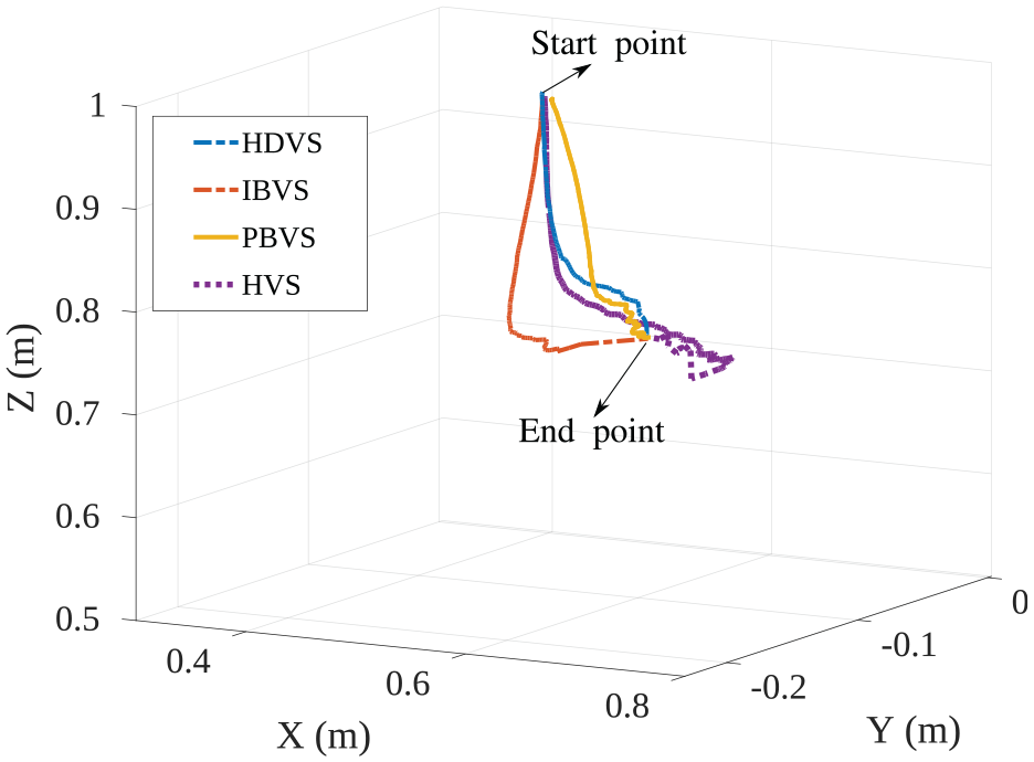
Comparison of EE trajectory for different methods in the real world.
Figure 10 suggested that shorter camera path is obtained for HDVS (blue path) than HVS (purple path) and IBVS (red path). To clarify, the distance travelled by the camera (robot’s EE) is 0.801 m in HDVS; however, this amount is 0.942 m in IBVS and 0.917 m in HVS. It should be mentioned that the most optimized Cartesian trajectory of the robot’s EE has been obtained by the PBVS method. The camera travelled distance is 0.722 m in this approach. As shown in Figure 10, IBVS (red path) showed the most unpleasant behaviour in the Cartesian trajectory of the EE, since the controller performs blind in the task space. Therefore, the robot in IBVS is more probable to move to joint limits and collide with the obstacles, especially when large rotations are required. PBVS (yellow path) performs well in the task space of the robot; however, it is sensitive to camera calibrations. Moreover, 3D estimation of the target must be calculated and be updated online at each computationally expensive iteration. In HDVS, the Z component is also separated from the image-Jacobian which avoids unnecessary motions in 3D. In addition, HDVS computations are faster than HVS. Therefore, HDVS is more suitable for online object tracking. Figure 11 illustrates feature errors of different approaches in VS for a similar assigned position of the Tag marker.
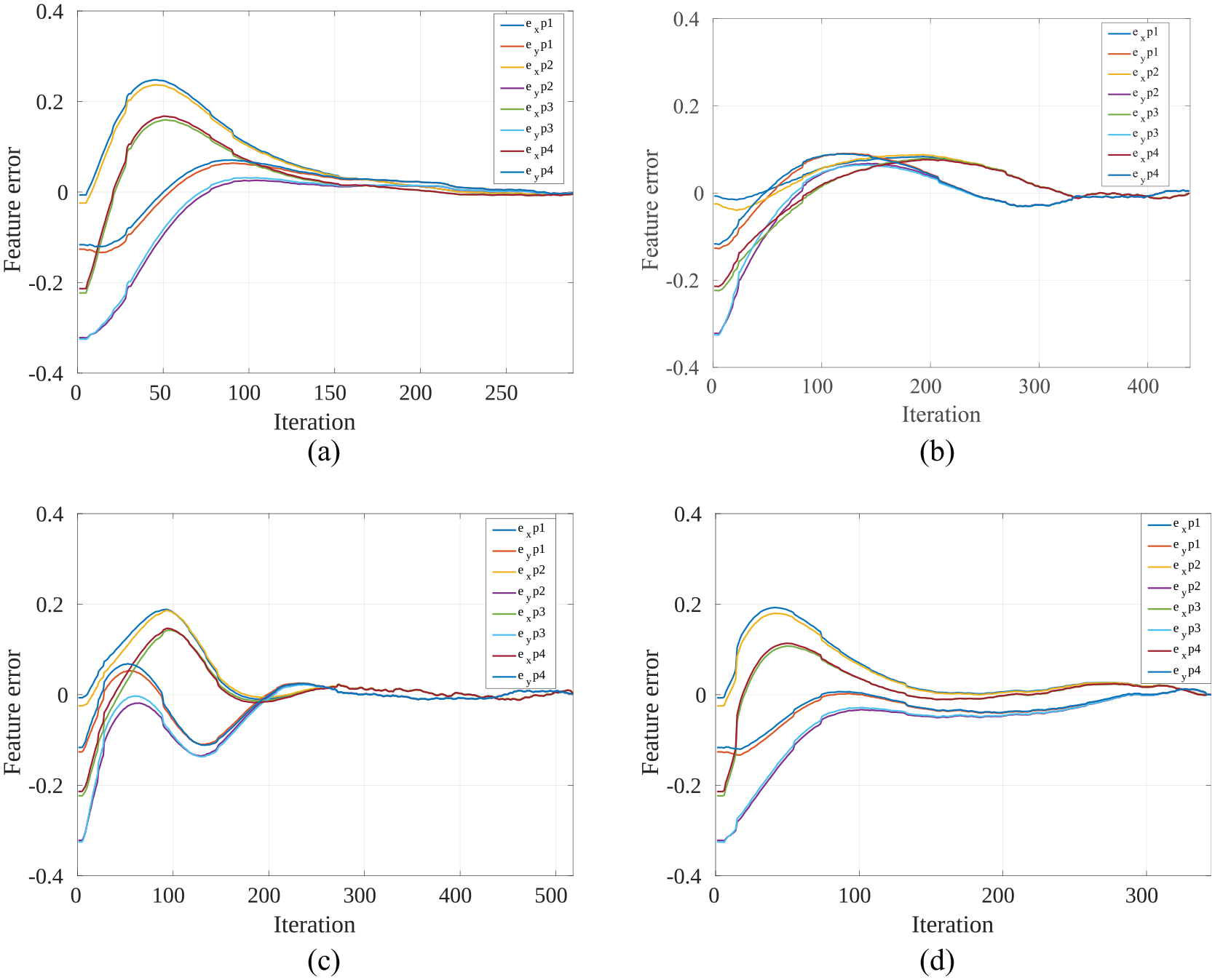
Comparison of feature errors for different methods in the real world: (a) PBVS, (b) IBVS, (c) HVS and (d) HDVS.
The RMSE is 0.021 in IBVS, 0.036 in PBVS, 0.032 in HVS and 0.024 in HDVS. In Figure 11(b), the IBVS represents the most optimized path in the camera frame, followed by HDVS. The RMSE in IBVS is less than other three methods. In Figure 11(b), the maximum feature error along the entire path is 0.089 which implies that there is a very low risk to lose the object from the camera screen. PBVS has the most unpleasant RMSE in camera screen than other methods (Figure 11(a)) as it performs blind in image screen. It is more probable in PBVS to lose the object from the camera fields of view since it has the highest feature error (0.24) compared to other counterparts. From Figure 11(c) and (d), it is clear that the HDVS method is faster (converged within 350 iterations) than HVS (converged within 510 iterations). Moreover, the convergence is more pleasant (fewer overshoots with same adaptive gains) and the RMSE is smaller in HDVS.
From Figures 10 and 11, it could be concluded that the proposed hybrid method has not necessarily the best behaviour in tracking the features in image space and Cartesian space (robot space), but it has an optimized behaviour in both. It comes from the fact that two components of camera velocities computed directly from the image space (translation in X and Y), while others computed from 3D reconstruction of the environment. Moreover, in HDVS, the object is less likely to be lost from the camera field of view than HVS and PBVS. This conclusion has been derived by comparing the maximum feature error in Figure 11(d), which is less than that amount in Figure 11(a) and (c). The bigger the error, the more it is probable to lose the feature from the camera field of view.
In Tables 1 and 2, a quantitative comparison of effective parameters in VS methods has been presented. Given that the quantitative amounts are obtained by the mean of 40 experiments with 10 different paths, repeated for all different methods in the same condition.
Comparison of visual servoing methods’ performance in image-plane.
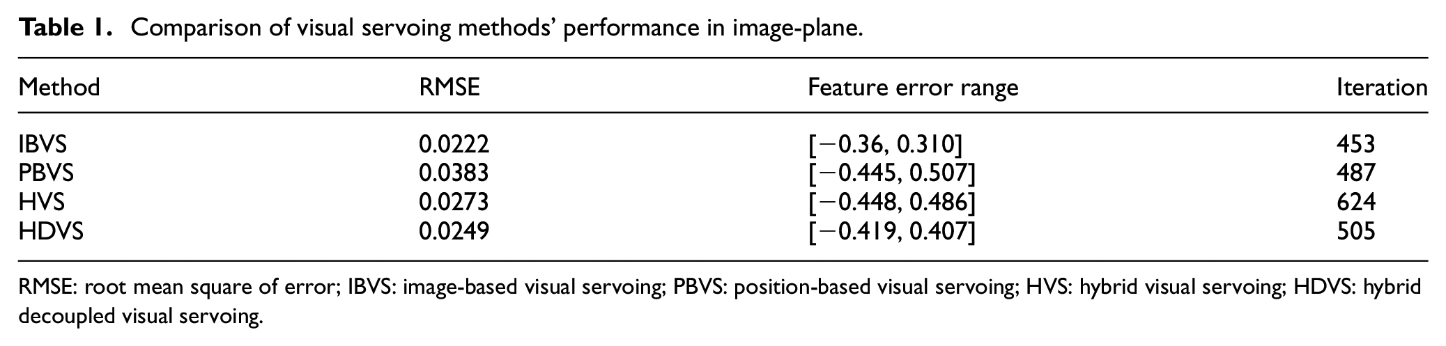
RMSE: root mean square of error; IBVS: image-based visual servoing; PBVS: position-based visual servoing; HVS: hybrid visual servoing; HDVS: hybrid decoupled visual servoing.
Comparison of visual servoing methods’ performance in Cartesian space.
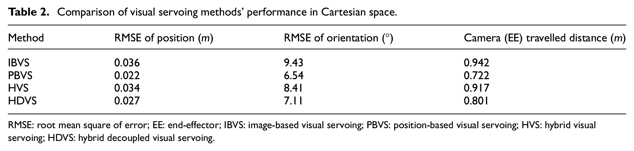
RMSE: root mean square of error; EE: end-effector; IBVS: image-based visual servoing; PBVS: position-based visual servoing; HVS: hybrid visual servoing; HDVS: hybrid decoupled visual servoing.
Looking at Table 1, the mean RMSE amount of HDVS is less than PBVS and HVS. As a result, HDVS performed better in image space than PBVS and classical HVS. Table 2 shows that the mean RMSE amounts of position and orientation in PBVS were less than their counterparts in the other three methods. Therefore, PBVS had the most optimized performance in Cartesian space. As it was expected, the performance of HDVS was better than IBVS and HVS in Cartesian space.
Another conclusion from Table 1 is that the feature error range in PBVS and classical HVS is bigger than HDVS. Therefore, the target is less probable to be lost from the camera screen in HDVS than the other two methods. Not to mention that HDVS performs faster compared to classical HVS, and fewer iterations are required to perform the same task. From Table 1, it can be seen that not only the IBVS has the smallest feature error range, but also has the smallest RMSE in comparison to other approaches. Assuredly, IBVS outperformed in image-plane if no singularity or local minima happen. However, the controller performs blind in Cartesian space (the highest RMSE for position and orientation in Table 2) and undesirable large camera motions often happen. All in all, in Cartesian space, HDVS suggests more optimized performance than IBVS and HVS (w.r.t. mean RMSE amounts presented in Table 2). In addition, HDVS performs more optimized than PBVS and HVS in image space (w.r.t. mean RMSE amounts presented in Table 1).
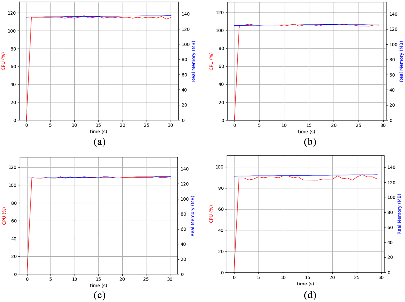
In Figure 12, the CPU and the RAM usage while different techniques are running has been shown. The comparison between the graphs in Figure 12 clearly illustrates our claim that HDVS is less computationally heavy compared to the other three methods. The CPU usage in HDVS is around 90%; however, this amount is above 105% for other techniques.
Comparison of CPU and RAM usage while each method is running in the real world: (a) PBVS, (b) IBVS, (c) HVS and (d) HDVS.
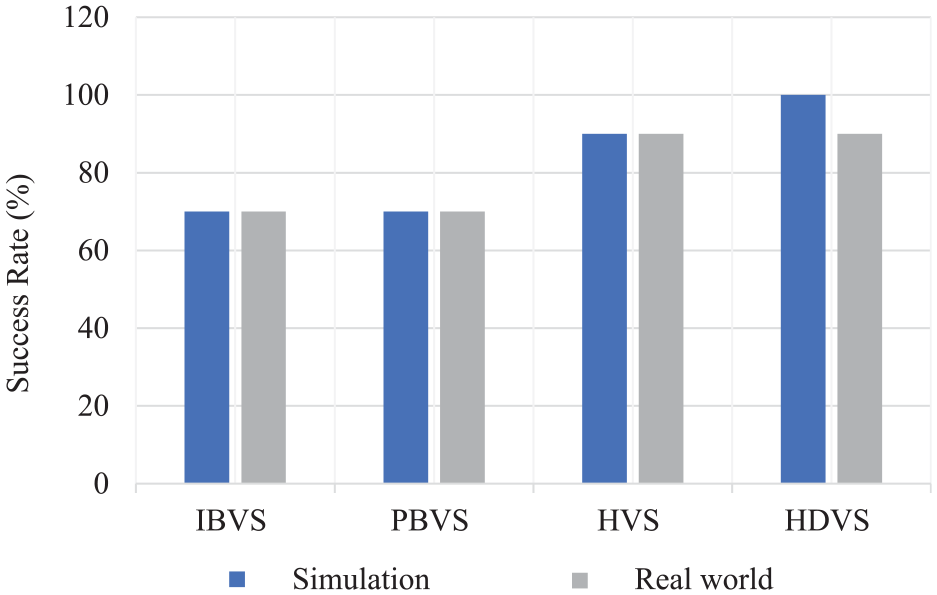
A qualitative comparison of the aforementioned results for all different methods is presented in Table 3. Table 3 illustrates that the proposed HDVS method offers an optimized trajectory both in Cartesian and image space. Furthermore, the controller is highly robust in terms of camera calibration (PBVS problem), image singularities (IBVS problem) and image noises (HVS problem). Not to mention that the proposed method has significantly relaxed the calculation, and the convergence speed is better than the classical HVS method. Figure 13 compares the success rate of four VS methods for 10 different random paths in simulation and their counterparts in the real world. From Figure 13, it can be concluded that HDVS outperformed with its success rate in both simulation (with 10 out of 10 successful trials) and real world (with 9 out of 10 successful trials) compared to other VS methods.
A qualitative comparison of visual servoing schemes.
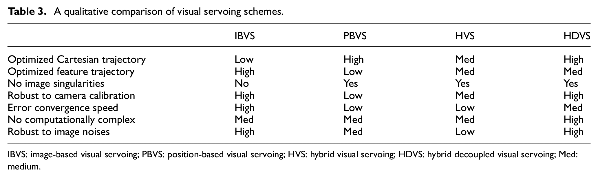
IBVS: image-based visual servoing; PBVS: position-based visual servoing; HVS: hybrid visual servoing; HDVS: hybrid decoupled visual servoing; Med: medium.
The success rate of four VS methods over 10 trials in the simulation and the real world.
Case study 5: Evaluating the performance of HDVS in tracking a moving object in the real world
In order to validate the results obtained from the simulation, a series of experiments conducted in the real world using a Franka robot arm. Both intrinsic and extrinsic calibrations of the camera have been accomplished using visual servoing platform (ViSP) libraries.
41
The adaptive gain parameters used in equation (20), where
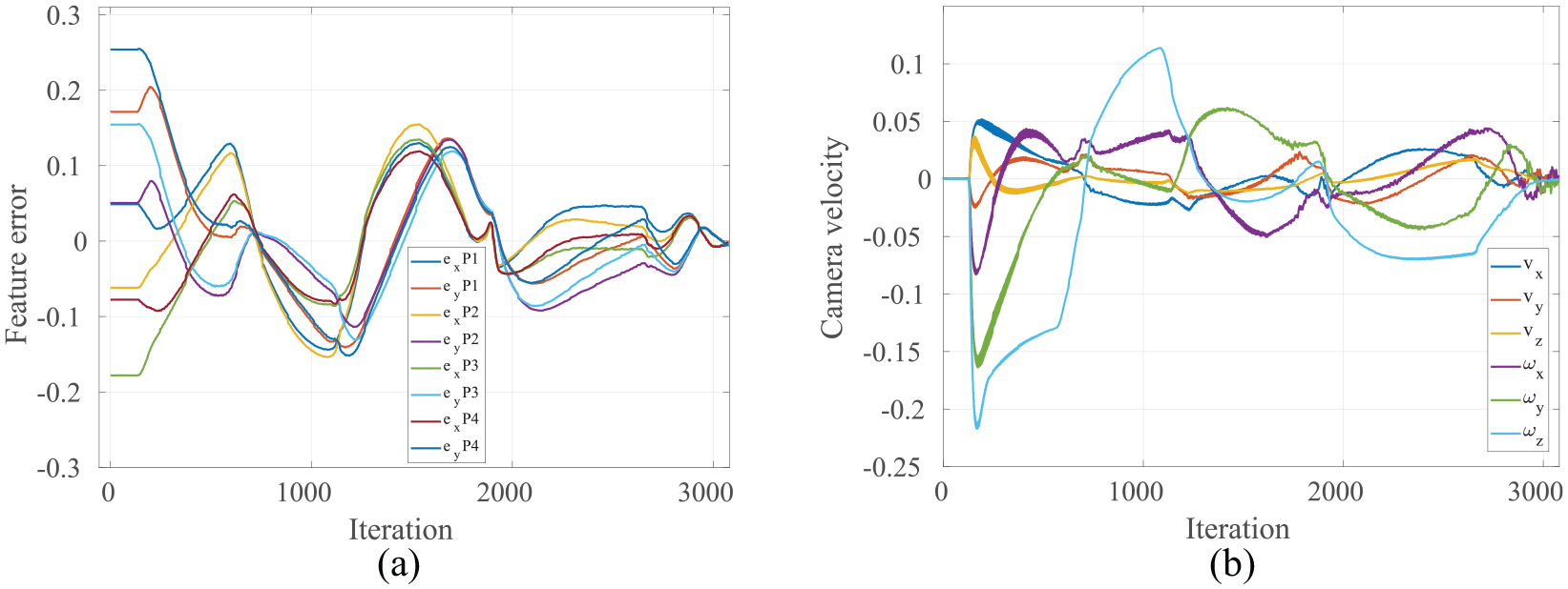
Analysing the performance of HDVS during tracking a dynamic object in the real world using a robot arm: (a) feature errors in HDVS and (b) camera velocity in HDVS.
Target is not static in this case study; therefore, there exist overshoots in the plots. The VS task was performed in 3100 iterations with RMSE of 0.074 along the entire path. In Figure 14(b), there is a peak in rotational velocity about Z-axis (iteration 100) which is created as a result of a pre-defined (90°) rotation. This large rotational velocity reveals that HDVS has a high capability in estimating the position of visual features in 3D. However, the error in the rotation could be interpreted wrongly as a translation error in Z-axis due to the camera retreat phenomenon in IBVS. Figure 15 compares the feature motions in image-plane for two HVS and HDVS methods.
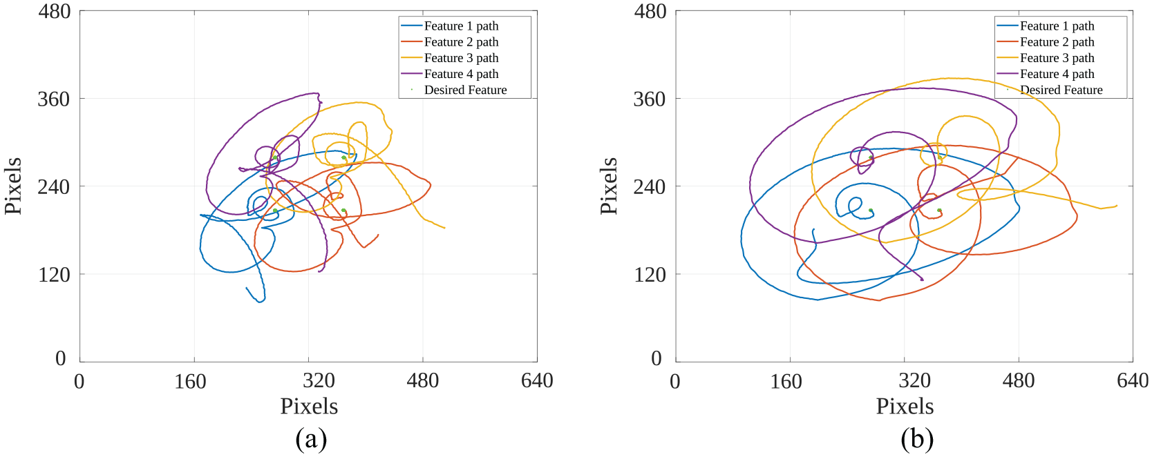
The trajectory of each feature to their desired ones, during the whole task of VS for (a) HDVS and (b) HVS techniques in the real world.
In Figure 15, green points denote the desired position of their corresponding features. Figure 15 suggested that the HDVS method (Figure 15(a)) aimed to keep the features closer to their desired positions than the HVS method (Figure 15(b)). This capability comes from the fact that the controller computes the translational velocities in the X-axis and Y-axis directly from the image-Jacobian while having explicit control over the rotations and translation in Z-axis. The motion of features implies that it is more likely to lose the points in the camera field of view by HVS than HDVS. Total image coordinates RMSE amount of 0.074 for HDVS and 0.1124 for HVS validates this claim.
Figure 16(a) and (b) shows the 3D trajectory of the robot’s EE generated by the HDVS and classical HVS controllers, respectively. HDVS controller offers a better performance in the task space than HVS. Total Cartesian position RMSE amount of 0.028 m for HDVS and 0.040 m for HVS, alongside total orientation RMSE of 6.388° for HDVS and 7.021° for HVS, declares this claim. Furthermore, the number of iterations to complete the task in HDVS is less than this amount in HVS. In this experiment, the number of iterations was 3078 in HDVS; however, this number was 3200 in the classical HVS method.
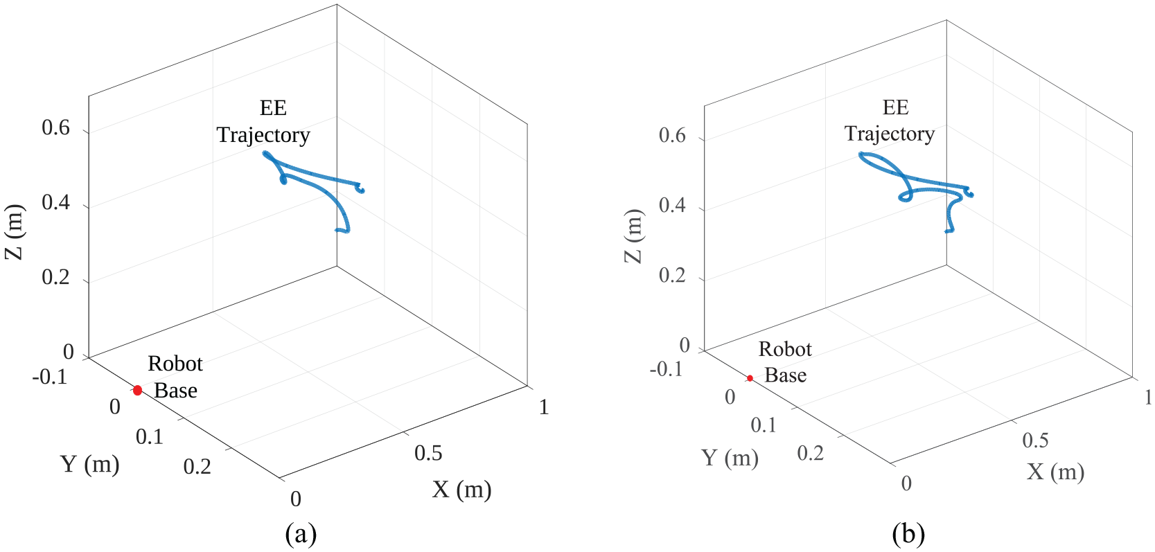
Three-dimensional trajectory of the EE in task space generated by (a) HDVS and (b) HVS in the real world.
Conclusion
In this article, a HDVS method has been proposed. This method has been developed to overcome the drawbacks of classical IBVS and PBVS methods and to improve the classical HVS method. In HDVS, all three rotations and translation in the Z-axis have been decoupled from the image-Jacobian. These four components’ errors will be regulated to zero by the 3D reconstruction of the visual features. Thereafter, a neuro-fuzzy LoLiMoT NN was used to approximate the pseudo-inverse of the proposed interaction matrix. Moreover, the convergence time was reduced with the help of adaptive gains rather than a constant gain. DLS method was applied in order to reduce the effect of robot singularities and to smooth the discontinuities.
The method not only has an optimized solution for the robot’s EE, but it also considers the optimized trajectories of features in the image space. Furthermore, HDVS has improved the performance of classical HVS in both image-plane and task space. The method is robust in terms of camera parameters and image noises, and it avoids singularities of the image-Jacobian effectively. In addition, it is less likely to lose the object from the camera fields of view than PBVS and HVS methods. Results obtained from 10 different random paths in simulation and their counterparts in the real world suggested 100% and 90% success rate in executing the VS tasks in simulation and the real world, respectively.
Thus, future work will be devoted to extend the LoLiMoT model domain to link feature errors directly to the joint velocities. Moreover, deep NNs could be used to function as feature extractions to overcome the complexities of feature selection.
Footnotes
Declaration of conflicting interests
The author(s) declared no potential conflicts of interest with respect to the research, authorship and/or publication of this article.
Funding
The author(s) disclosed receipt of the following financial support for the research, authorship and/or publication of this article: This research was conducted as part of the project called ‘Reuse and Recycling of Lithium-Ion Batteries’ (RELIB). This work was supported by the Faraday Institution (grant no. FIRG005).
Data availability statement
The data that support the findings of this study (the simulation in Gazebo/ROS, C++ codes and demo clip) are openly available in Figshare (![]() ) with doi (10.6084/m9.figshare.12980009.v1).
42
) with doi (10.6084/m9.figshare.12980009.v1).
42
References
Supplementary Material
Please find the following supplemental material available below.
For Open Access articles published under a Creative Commons License, all supplemental material carries the same license as the article it is associated with.
For non-Open Access articles published, all supplemental material carries a non-exclusive license, and permission requests for re-use of supplemental material or any part of supplemental material shall be sent directly to the copyright owner as specified in the copyright notice associated with the article.