
Abstract
There is growing interest in recycling and re-use of electric vehicle batteries owing to their growing market share and use of high-value materials such as cobalt and nickel. To inform the subsequent applications at battery end of life, it is necessary to quantify their state of health. This study proposes an estimation scheme for the state of health of high-power lithium-ion batteries based on extraction of parameters from impedance data of 13 Nissan Leaf 2011 battery modules modelled by a modified Randles equivalent circuit model. Using the extracted parameters as predictors for the state of health, a baseline single hidden layer neural network was evaluated by root mean square and peak state of health prediction errors and refined using a Gaussian process optimisation procedure. The optimised neural network predicted state of health with a root mean square error of (1.729 ± 0.147)%, which is shown to be competitive with some of the most performant existing neural network–based state of health estimation schemes, and is expected to outperform the baseline model with ∼50 training samples. The use of equivalent circuit model parameters enables more in-depth analysis of the battery degradation state than many similar neural network–based schemes while maintaining similar accuracy despite a reduced dataset, while there is demonstrated potential for measurement times to be reduced to as little as 30 s with frequency targeting of the impedance measurements.
Keywords
Introduction
Recent years have seen a rapid increase in the number of electric vehicles (EVs) in circulation. 1 Owing to the use of high-value materials, such as cobalt and nickel, there is a strong economic, environmental and political case to implement solutions for recycling and re-use end of life EV batteries based on lithium-ion technology.1–3 Such batteries have, for the most part, exhausted their useful life for re-use in EVs, however have demonstrably useful applications in repurposed static energy storage systems and represent a large body of energy storage capacity.1,4 It is necessary, however, to properly assess the battery condition and degradation to inform the appropriate re-use applications or, if necessary, subsequent recycling. 3 The re-use of batteries for a second life application presents a further requirement to properly match batteries of similar condition in a given energy storage system to prevent unbalanced degradation by over (dis-)charging,4,5 which can reduce its remaining useful life (RUL).
A quantity of particular interest for characterisation of batteries is the battery state of health (SoH), typically defined from measurements of the battery capacity for lithium-ion batteries (LIBs). Typically cells with greater than 80% of their rated capacity are considered for re-use in EV applications,4–6 while below this threshold, cells with as little as 65% of their original capacity are suitable for second-life applications. Currently, cell capacity is determined by discharge testing which takes several hours, making it a time consuming, and hence costly process. 7 Electrochemical impedance spectroscopy (EIS) is a promising technique that provides insight into the battery condition through exposing the changes in parameters pertaining to the battery internal resistance and electrochemical properties, and has presented considerable improvements in measurement times. These qualities justify its extensive prior applications in investigation of battery condition8–11 and SoH.12,13 It has been demonstrated through equivalent circuit (EC) modelling of the impedance response of cells that the charge transfer resistance extracted from EIS measurements is a useful indicator of SoH 13 ; however, a principal limitation is that individually such parameters do not always vary significantly or linearly with the battery age, 14 and therefore it is suggested that these approaches are inadequate for SoH estimation in this case.
Recent years have seen exploration of numerous machine learning schemes to estimate SoH.12,15–18 Neural networks (NNs) in particular are an attractive solution to SoH estimation in that they can model complex, non-linear systems with cross-interactions between system variables without a detailed underlying theoretical framework of the system being considered. 12 This is useful for LIBs where the precise internal composition and design is often commercially sensitive and hence not accessible. Nonetheless, to the authors’ best knowledge, very few prior works have developed an NN-based SoH estimation scheme using such extracted parameters directly from EIS as predictors for the SoH.
In this study, an NN-based approach for estimation of the SoH from impedance measurements of Nissan Leaf 2011 battery modules is presented. This study aims to replicate the successes of prior, high-accuracy NN-based approaches, while addressing their primary limitations, namely, model complexity, large required training dataset size and lack of physical parameters extracted that pertain to the battery condition. Hence, the expected contributions of this work are as follows:
High-accuracy estimation of SoH with a reduced training dataset of 106 samples, with an average estimation error below 3%.
Consideration of parallel battery arrangements in contrast to focus on single cell SoH estimation in similar studies.
The proposal of an optimised equivalent circuit model (ECM) parameter-based NN model using hyperparameter optimisation, which is not explicitly considered in most works.
Greater insight into the battery degradation due to use of an ECM approach than available with schemes monitoring evolution of battery current/voltage.
Background and related works
The problem of state measurement of LIBs has been widely studied, most notably for estimation of the battery state of charge (SoC), while literature pertaining to SoH estimation remains less prevalent. Focuses of recent works in the area of SoH estimation have included incremental capacity (IC)/differential voltage (DV) measurement, 19 Coulomb counting, 20 (dual) extended Kalman filters21,22 or empirical health degradation models such as those developed by Perez et al. 23 However, the bulk of literature pertaining to SoH estimation focuses on prognostics and health management of existing battery systems, 24 with less emphasis placed on end of life characterisation of batteries. Furthermore, a majority of SoH estimation works focus on single cells. This presents a problem in the EV application, where cells are often built up in parallel to form battery modules. In Chang et al., 25 the problem of capacity estimation of parallel battery arrangements based on discharge current curves was studied, with the benefit of being validated across multiple cell chemistries. However, although this approach effectively reduced measurement times by the requirement for only a single discharge cycle, this does not eliminate the requirement to perform a discharge test entirely.
EIS
EIS represents an advanced characterisation tool for investigation of the ageing state of batteries. Studies of LIBs using EIS are various, with applications including quality control,
26
investigation of battery ageing mechanisms11,27–29 and estimation of battery SoC and SoH.13,30 The principle of operation of EIS is to sample the impedance of a cell at a range of discrete frequencies by applying a probing periodic voltage (potentiostatic) or current (galvanostatic) signal,
26
measuring the voltage or current response of the cell across a working electrode and calculating the impedance
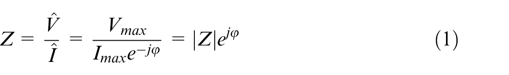
given the maximum current and voltage
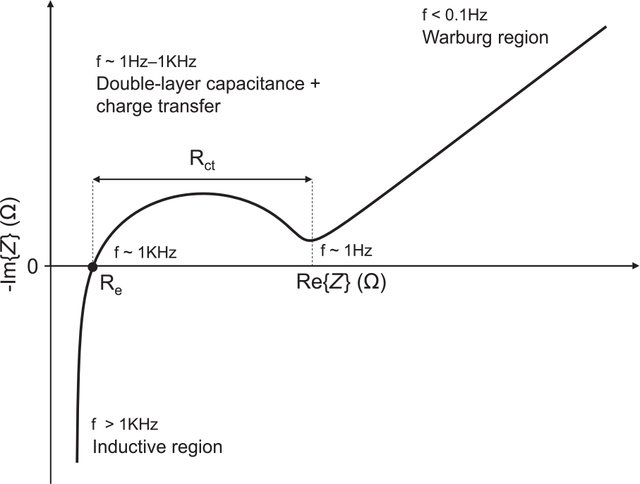
Idealised EIS Nyquist plot for a lithium-ion cell. The different loss mechanisms, high to low frequency (left to right) are inductive, resistive, capacitive and diffusional (Warburg impedance).
The latter, EC modelling, presents a simple, yet effective picture of the battery condition by considering the structure of the battery impedance response, defined by the internal electrical and kinetic processes occurring within the cell and associating these with one or more elements in an EC describing the system. A simple ECM for LIBs is the Randles cell (Figure 2), comprising a resistor
where
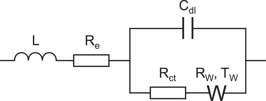
The Randles cell equivalent circuit model (modified with an inductor to match Figure 1), comprising a pair of resistors
For SoH estimation with EIS, a principal issue is the limitation that results depend not only on the cell ageing state, but also on the cell’s SoC, temperature and even the nature of the electrical connection between the cell and measurement equipment,6,30,36 making reproduction of results difficult. Quantification or removal of these dependencies has been the focus of numerous works, including investigations of cells at 0% SoC,
33
while a combined study of the variation of the impedance characteristics of LIBs with temperature, SoC and ageing with EIS was first carried out by Waag et al.
9
This is more comprehensively addressed by Wang et al.,
13
leveraging this to develop an estimation function for the SoH of a lithium iron phosphate (LFP) cell based on a linear regression of the charge transfer resistance (
Machine learning for SoH estimation
Data-driven approaches such as machine learning have been widely studied for the development of prognostic, health management and health estimation models for a range of systems. For example, data-driven approaches have been applied with success in the related area of bearing fault diagnosis and prognostics,37,38 where it is often impractical to develop precise health degradation models to predict their RUL. Similarly for studies of LIBs, a number of data-driven estimation models for the battery SoC,15,39,40 SoH12,15–18,41 and RUL have been developed.12,42,43 Many of these studies focus on online estimation of SoH by capacity, with the prevailing approach involving following the evolution of the current, terminal voltage and partial capacity curves of the battery with time as applied by previous works.17,18,43 These approaches have the potential to provide rapid SoH estimation; for example, 17 applied an artificial neural network (ANN)-based classifier on features extracted from fixed time windows of as little as 60 s. In the case of Bonfitto et al., 17 this is achieved with low computational complexity; however, a limitation is that it is based on classification into discrete SoH bands of 5% and hence is limited in precision. On the other hand, Shen et al. 18 used deep convolutional neural networks (DCNNs) with transfer and ensemble learning with demonstrably high accuracy and precision, but with greatly increased computational complexity.
Other models based on recurrent neural networks (RNNs) focus on time series forecasting of the battery state. Such an approach is applied in Eddahech et al. 12 monitors the degradation of capacity and internal resistance with time to develop a high-accuracy SoH degradation model. More recently, similar approaches have been explored based on the RNN principle by monitoring the cell current and terminal voltage, including application of the gated recurrent unit (GRU) RNN by Jiao et al. 39 and long short-term memory (LSTM) in Mamo and Wang 40 for the related problem of SoC estimation, as well as a modified LSTM in Li et al. 43 for estimation of SoH. Generally, the RNN-based approaches are capable of predicting the battery states with outstanding accuracy and can be extended in the case of SoH to predict the evolution of the battery condition for estimation of RUL as in Eddahech et al. 12 and Li et al. 43 However, being suited for state monitoring, a key limitation is the sensitivity of model predictions to the previous battery state, which makes these approaches unsuitable for characterisation of most end of life batteries.
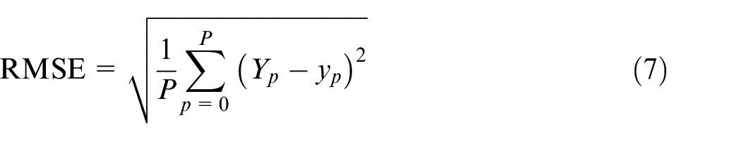
For non-RNN-based approaches, typical root mean square (RMS) prediction errors for NNs range between 1% and 5%, while some approaches such as those by Kim et al. 41 and Liu et al. 44 are shown to achieve even greater capacity prediction performance. The high prediction accuracy is achieved based on application of highly complex NN models, with the caveat that as the number of neurons used to model the system increases, there is a larger requirement for training data to prevent over-fitting of the network to the training dataset, while the model becomes more computationally demanding due to the increased number of model parameters. 17
Most critically, it has been noted 6 that a principal limitation of many of these NN studies is the lack of detailed information regarding the battery ageing state, such as that exposed by the extraction of ECM parameters from EIS. Few approaches have been explored with an NN-based scheme to estimate cell SoH directly using ECM parameters, with prior studies proposing an extreme learning machine (ELM) monitoring the evolution of ECM parameters as SoH predictors with cell cycling 15 or a single hidden layer feed-forward NN 16 based on ECM parameters extracted with hybrid pulse-power characterisation (HPPC). The accuracies for these approaches lie with RMS prediction errors between 2.4% and 5%, ultimately suggesting there is scope for further study and improvement in this area. Beyond the ECM approach to battery modelling, more generalised approaches such as fuzzy c-regression have been introduced for parameter estimation of non-linear systems by Jabeur Telmoudi et al. 45 and later extended to modelling batteries in Telmoudi et al. 46 in which a fuzzy c-regression model with Euclidean particle swarm optimisation is employed to build a model of an NiMH battery under cycling, which is used to estimate SoH with high accuracy. However, although such methods are capable of modelling the battery behaviour with potentially higher accuracy than an ECM-based approach, it is unclear how these parameters are related to physical degradation phenomena occurring within the cell.
Data library
A library of impedance spectra and corresponding discharge capacities was used for the present study, measured from a series of 13 battery modules from an end of life Nissan Leaf 2011 battery pack to obtain a realistic representation of the end of life battery condition. Each module is arranged in a 2P-2S configuration with three terminals – red, white and black – with each parallel arrangement of two cells accessible by measurement across the red and white and black and white terminals, respectively. For each parallel arrangement of cells, occupying a combined capacity range of 50–55.5 A h (77%–85% SoH) impedance data were collected at room temperature (
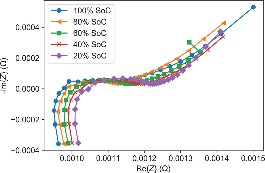
Experimental impedance data obtained at 25 °C, frequency range 1 kHz–15 mHz over the red and white terminals of module 1 of 13, capacity 54.9 A h and variation with battery state of charge (SoC).
Methodology
The present work aims to develop an NN model of the SoH of end of first life EV batteries by estimation of the discharge capacity. This is proposed based on their impedance characteristic measured by impedance spectroscopy, from which physical parameters pertaining to the battery condition may be extracted by fitting to an ECM. In this case, the SoH was considered to be the ratio of the battery discharge capacity to the original rated battery capacity, as this forms the basis of typical screening criteria for end of life batteries. Using these parameters, a simple baseline model with low computational complexity is first proposed to estimate SoH before the arguments and methodology for refining the model to increase accuracy are presented.
Parameter extraction
As previously mentioned, NNs are excellent at learning the behaviour of non-linear systems, cross-interaction between system variables and existing patterns in the data used to train the network. While this is the case, it often requires large amount of data to learn general patterns in the data to generalise well to new problems. Since the goal of this study is to work with a dataset smaller than considered in other studies, it is necessary to extract features from the dataset that have a well-defined relation to the desired output (SoH). An ECM-based method for parameter extraction fits this problem well due to the well-documented relationship between the equivalent series and charge transfer resistances (
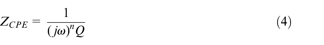
where the capacitance
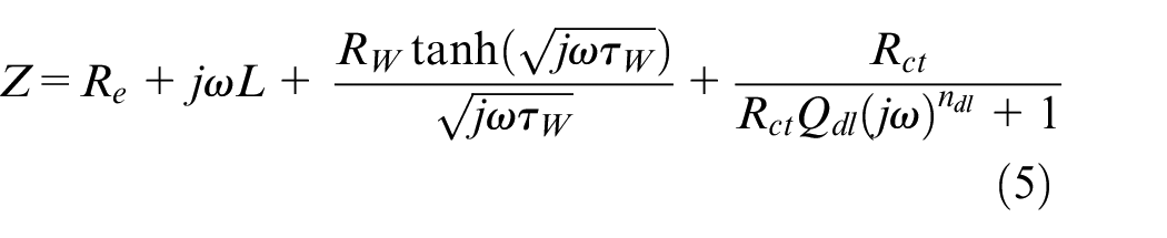
where
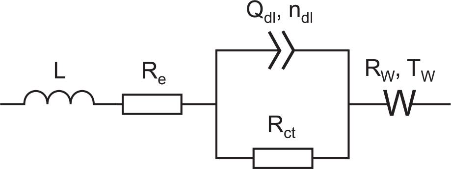
Diagram of the modified Randles circuit used as an equivalent circuit model (ECM) to describe the impedance response of the cells used in this study. The ECM parameters associated with each element are listed, respectively.
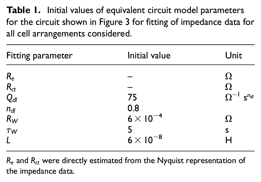
Initial values of equivalent circuit model parameters for the circuit shown in Figure 3 for fitting of impedance data for all cell arrangements considered.
The SoH ground truth values were then taken to be the ratio of the measured discharge capacity
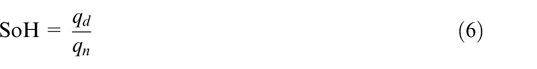
where
Baseline model
To estimate the SoH of the cells using the extracted parameters, a feed-forward NN approach is proposed as a baseline method as shown in Figure 5. Development and training of the NN model was performed in Python using the publicly available machine learning libraries Keras and TensorFlow 2
48
on an NVIDIA GTX 1060 6-GB GPU using the Adam
49
optimiser. The model weights were initialised with a Glorot uniform scheme, with the sigmoid hidden layer activation function, an optimiser learning rate of 0.01 and no output layer activation function. To test the accuracy of the NN model, the dataset was partitioned according to a K-fold cross-validation scheme. K-fold cross-validation is a commonly used technique to achieve more reliable indicators of NN performance with smaller datasets50,51 and involves shuffling the dataset prior to splitting into
for each SoH value
while the SoH ground truth values were normalised as
where
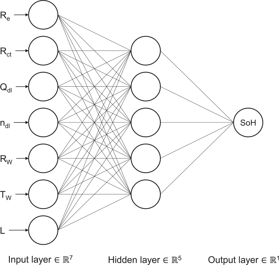
Diagram of the baseline feed-forward neural network architecture using extracted equivalent circuit model parameters as predictors for the battery state of health.
NN optimisation
It is well documented that to achieve the best NN prediction performance for a given problem, it is necessary to consider the choice of so-called network ‘hyperparameters’. For a given model, the hyperparameters include the number of neurons present in each hidden layer, the number of hidden layers and the ‘learning rate’ of the optimiser used to control the magnitude of updates to the network weights and biases. Over-fitting to the training data is a critical problem when dealing with small datasets, so it is necessary to find a balance between developing a model that is sufficiently complex to find generalised patterns in the data, such that it generalises well to an unseen dataset, and limiting over-fitting by preventing the network from adapting to patterns specific to the training data, such as noise, thus hampering its generalising power. To achieve this, the full dataset was first split into six folds as previously with a single fold held out for testing, the remaining folds forming an ‘inner’ dataset. A Gaussian process (GP) optimisation algorithm introduced by Pedregosa et al.
52
was used to minimise a cost function, which in this case is the associated RMS prediction error from a fivefold cross-validation process on the five ‘inner’ folds. This cost function was evaluated with respect to the chosen hyperparameter combination in a search space detailed in Table 2. Many of the hyperparameters are self-explanatory; however, in this case, a categorical hyperparameter was included describing the NN shape. The shape controls the number of neurons in each hidden layer based on the number of neurons in the first hidden layer. For the ‘funnel’ structure, the number of neurons in the kth hidden layer
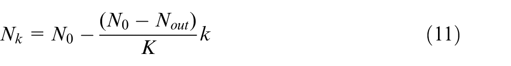
rounded to the nearest integer (half to even) where

The hyperparameter search space used to optimise the neural network performance.
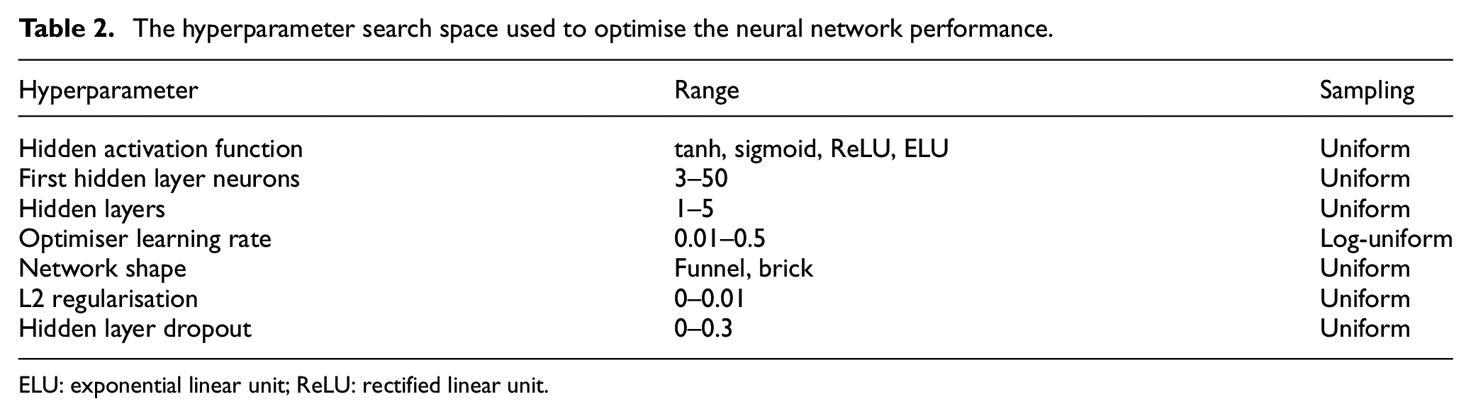
ELU: exponential linear unit; ReLU: rectified linear unit.
The hidden layer dropout hyperparameter represents the fraction of neuron outputs from each layer that are set to zero during the training process to prevent over-fitting.
For the GP estimator for the cost function, the Matérn covariance function was used, defined as
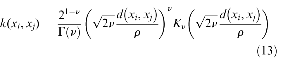
with
This surrogate function was used to guide 250 additional evaluations of the cost function by evaluating at the point with the minimum negative expected improvement, probability of improvement and lower confidence bound acquisition functions. In this way, convergence to the model with the lowest prediction error is achieved much more rapidly than the simpler random search or grid search of hyperparameters. Once the optimal cost function was found, a new model was generated with the resulting hyperparameters and evaluated on the held-out sixth test fold. This process was repeated six times for all six original folds. Finally, the combination of hyperparameters that achieved the lowest RMS prediction error on its test set was chosen to generate the final NN model used to estimate SoH for this study. Once the optimised model has been generated, the overall SoH estimation procedure based on the resulting SoH model is shown in Figure 6.
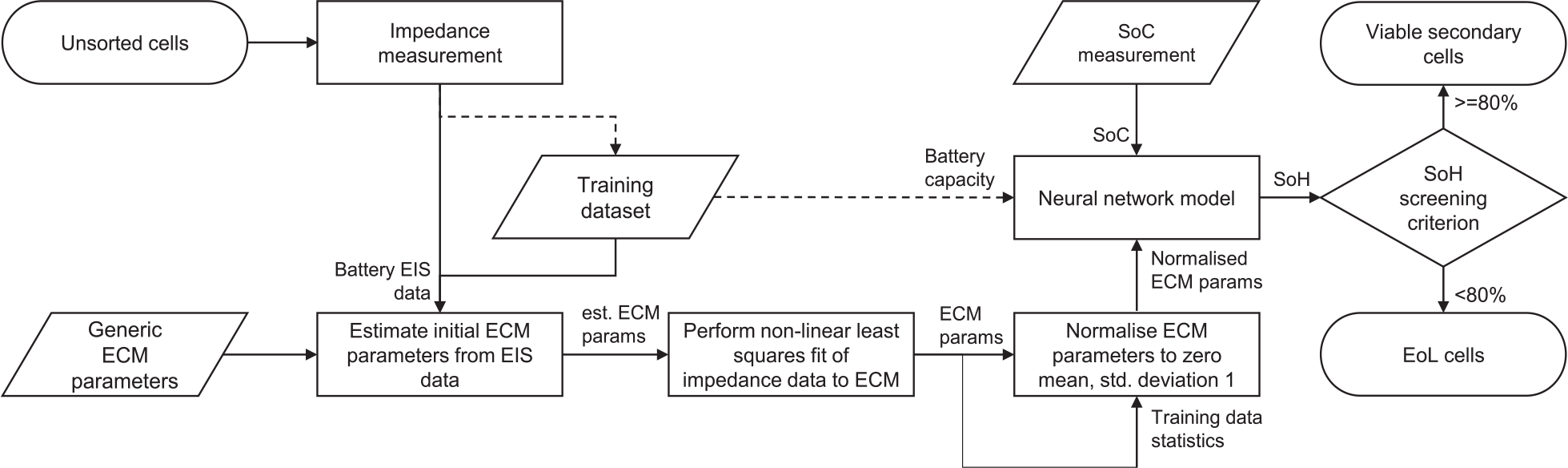
Block diagram of the overall SoH estimation procedure using the proposed neural network model.
Results and discussion
To evaluate the effectiveness of this SoH estimation scheme, the results of the parameter extraction method, hyperparameter optimisation and comparison with the baseline model are presented here. The proposed SoH estimation scheme is compared with a range of alternative machine learning schemes, including commonly used techniques as well as approaches specific to similar studies addressed in the related works. Finally, the performance of the scheme is assessed in the context of reducing measurement times by considering the model performance on a reduced frequency range dataset.
ECM fit
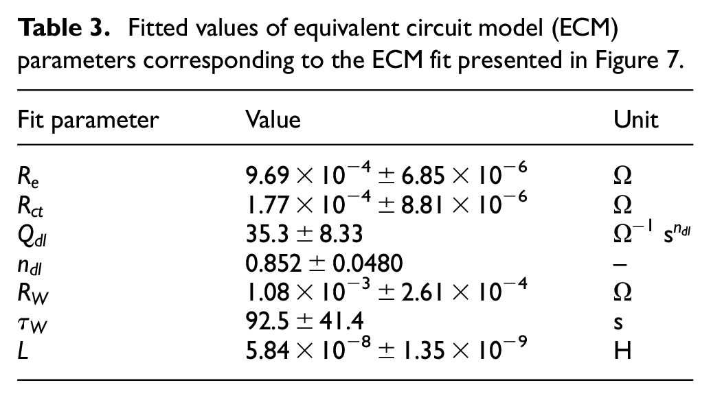
Figure 7 shows an impedance spectrum from the dataset considered in this study over the red and white terminals of module 1 of 13 with capacity 54.9 A h, obtained at 60% SoC, 25 °C over the frequency range 1 kHz–15 mHz. This has been fitted to the modified Randles circuit in Figure 4 with the resulting fitted parameters presented in Table 3. Here, the form of the ECM used is justified by the presence of a capacitive loop present in the medium frequency range, which was attributed to be due to the double-layer capacitance and charge transfer reactions at the electrodes. A deviation from ideal capacitive behaviour is observed in the depression of the loop and slight shift of high-frequency phase away from 90° 35 and hence justifies the substitution of the double-layer capacitance in the Randles circuit for a constant phase element describing this deviation from ideality.30,35 The presence of a tail on the spectrum at high frequencies reaching into the positive imaginary range is indicative of inductive behaviour. Finally, at low frequencies, the characteristic Warburg region is observed. The ECM used is shown to fit well to the capacitive region of the spectrum; however, deviations from the expected Warburg behaviour are observed at low frequencies. The fit could be improved by inclusion of further ECM elements; however, this complicates the fitting process by introducing greater uncertainty of the values of the fitting parameters due to the low information content of the impedance spectrum. 27
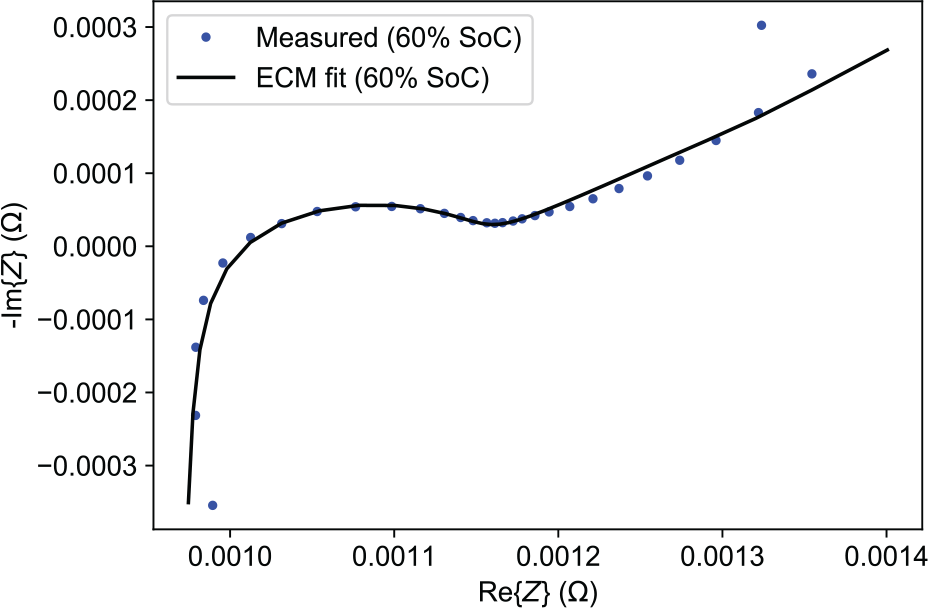
Nyquist plot of fit to equivalent circuit model shown in Figure 4 with experimental impedance data obtained at 60% SoC, 25 °C, frequency range 1 kHz–15 mHz over the red and white terminals of module 1 of 13, capacity 54.9 A h.
Fitted values of equivalent circuit model (ECM) parameters corresponding to the ECM fit presented in Figure 7.
Hyperparameter optimisation
As previously discussed, it is necessary to consider the hyperparameters of a given NN model to achieve the best accuracy. Figure 8 shows the results of the hyperparameter search, with the partial dependence of the RMS prediction error with respect to each hyperparameter shown on the diagonal, and contour plots of the partial dependence surface over each pair of hyperparameter values, which show higher and lower prediction errors in the darkened (blue) and pale (yellow) regions, respectively. The partial dependence plots between two hyperparameters were computed by evaluating the surrogate function 250 times at 40 points in hyperparameter space with all other hyperparameters chosen randomly. The average result of this process is computed, such that the dependency plots represent the average behaviour of the cost function as any given two hyperparameters are varied. The black points for a given combination of hyperparameters correspond to a full evaluation of the cost function, with the found optimal model represented by the pale (red) point.
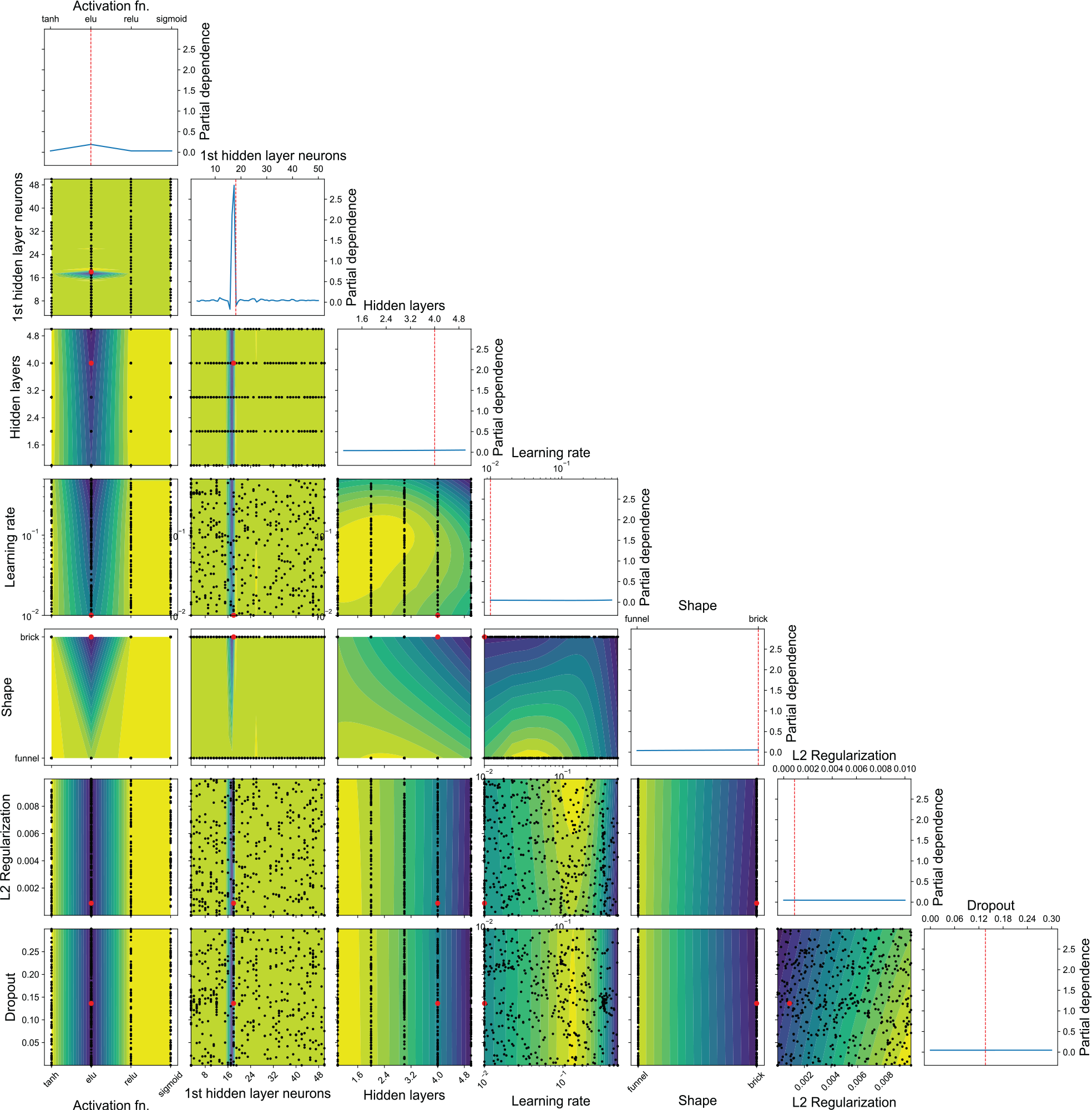
Result of hyperparameter optimisation showing partial dependence of RMS prediction error with each hyperparameter. Each point represents the average over a sixfold cross-validation trial of the neural network generated with the corresponding hyperparameters.
As shown, there is very little dependence of the network performance on average with each hyperparameter individually, with most of the dependency information encoded in the cross-interactions of different hyperparameters. When considered with other hyperparameters, there is a bias towards low, but nonzero learning rates as expected, with the optimum around 0.1 as a balance between convergence speed and stability, while the cost function is shown to slightly decrease for models with high numbers of hidden layers and models with the ‘brick’ structure as the amount of L2 regularisation penalty is increased. On a superficial level, there is a bias towards models with fewer hidden layers when considered with most hyperparameters, suggesting models of high complexity are ineffective at accurately predicting SoH with the size of dataset considered. However, a large number of cost function evaluations guided by the surrogate function were focused on models with around 17 hidden layer neurons, 3–5 hidden layers with the exponential linear unit (ELU) activation function. Furthermore, the location of the optimum of the cost function in hyperparameter search space was found to significantly diverge from that used for the baseline model, highlighting the deficiency of the simpler baseline model for this problem.
The resulting optimised NN structure is shown in Figure 9 with corresponding hyperparameters in Table 4. In this case, the model achieved an RMS fivefold cross-validation error of 1.630% on the ‘inner’ validation dataset, and 1.733% on the single held-out test fold. It is demonstrated that the model structure is significantly enlarged, with quadruple the number of hidden layers in spite of the small dataset size used, which is divergent from the approaches applied by Densmore and Hanif 15 and Yang et al. 16 based on ECM parameters. For the optimised NN model, the convergence during training to a minimum mean squared prediction error was recorded over the number of training epochs for the training and validation dataset partitions, and is presented in Figure 10. The model shows rapid convergence in the first 50 epochs, with little reduction in validation error over ∼350 epochs before early stopping at ∼380 epochs. The training and validation errors in this case are well matched and show little to no divergence over continued training, while the inverse is widely recognised as an indicator of model over-fitting. 51
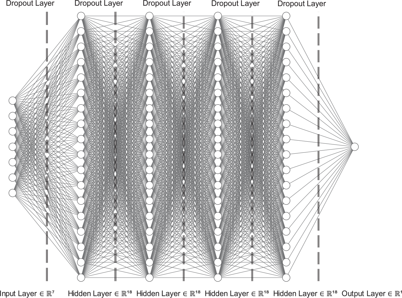
Optimised neural network structure generated from the hyperparameter optimisation scheme.
The optimised neural network hyperparameters corresponding to the network structure in Figure 9.
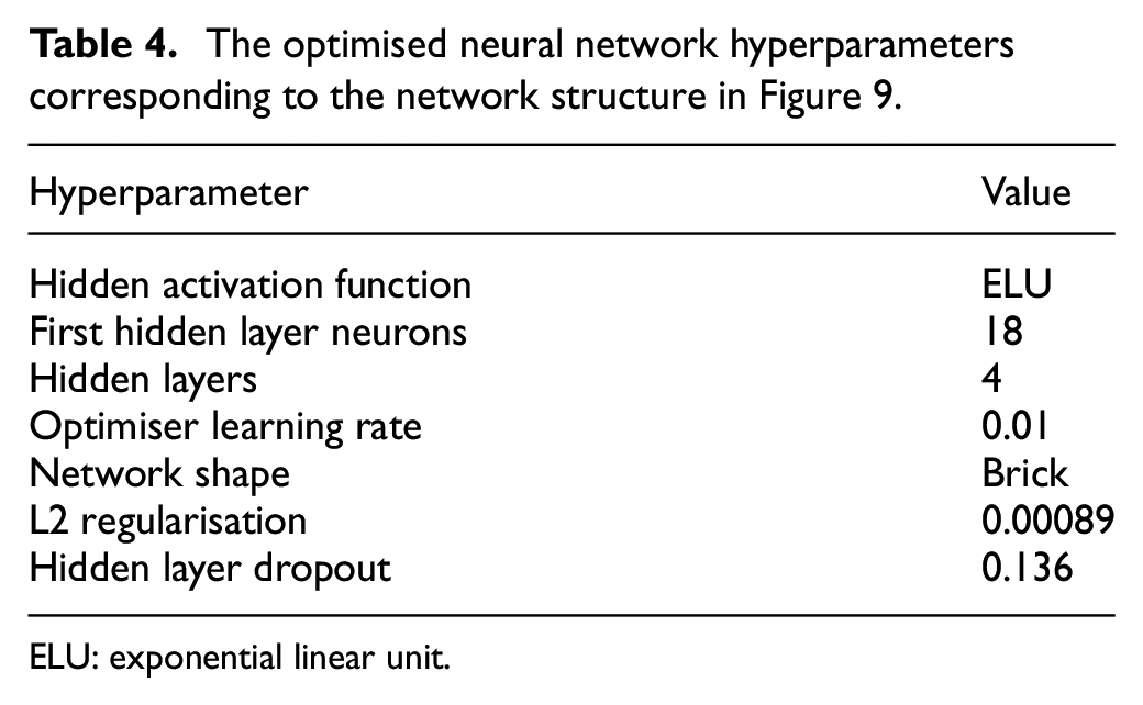
ELU: exponential linear unit.
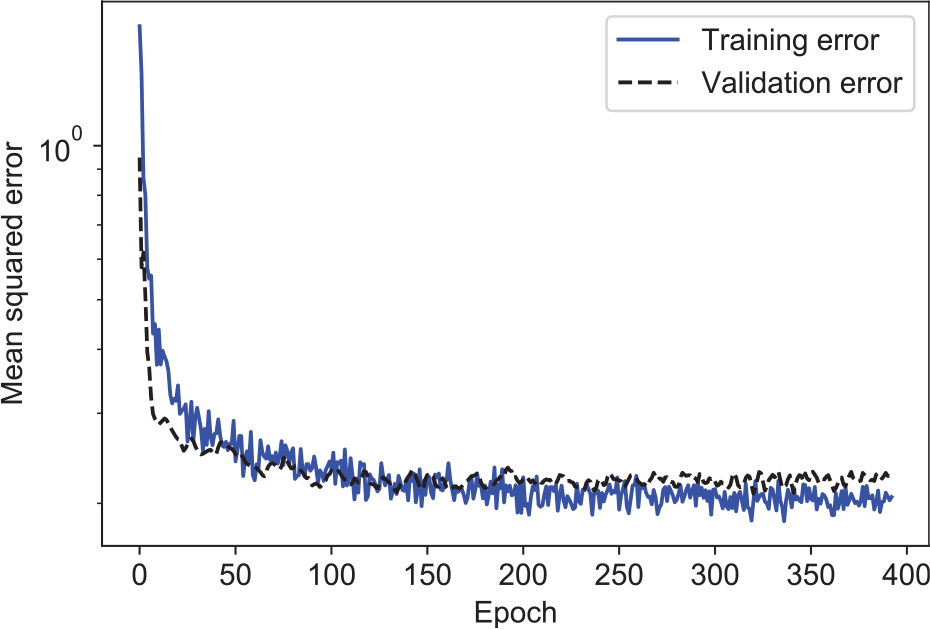
Convergence of the neural network model by reduction of RMS state of health prediction error with number of training epochs. Training and validation errors are well matched suggesting no over-fitting of the training data.
Using the sixfold cross-validation scheme, the RMS, MA and peak prediction errors for the baseline model were generated as a benchmark to compare with the performance of the optimised model. This comparison is summarised in Table 5. The results show that the hyperparameter optimisation provides a clear benefit over the baseline model, with significant improvements to RMS (0.403%) and MA (0.548%) error, while the lower standard deviation on these errors suggests that the optimised model generalises more consistently to unseen data. Little to no difference in peak error over the six trials was recorded, suggesting that while the optimised NN predictions are on average more accurate, there is little reduction in potential outlier predictions generated by the optimised network. This comparison is illustrated in Figure 11, showing graphically the distribution of predictions between the two models. A further comparison between the baseline model and the optimised model is presented in the variation of network accuracy with the number of training samples used in Figure 12. Each point represents the sixfold cross-validated RMS prediction error of each model averaged over 10 runs in total. From the graph, it is clear that the optimised model begins to outperform the baseline for training datasets of greater than around 50 samples, with the cross-over point at 43 samples. Overall, this demonstrates the greater generalising power of the optimised model over the baseline.
Sixfold cross-validated RMS, mean absolute (MA) and peak prediction errors of state of health estimation for the baseline and optimised neural network model.
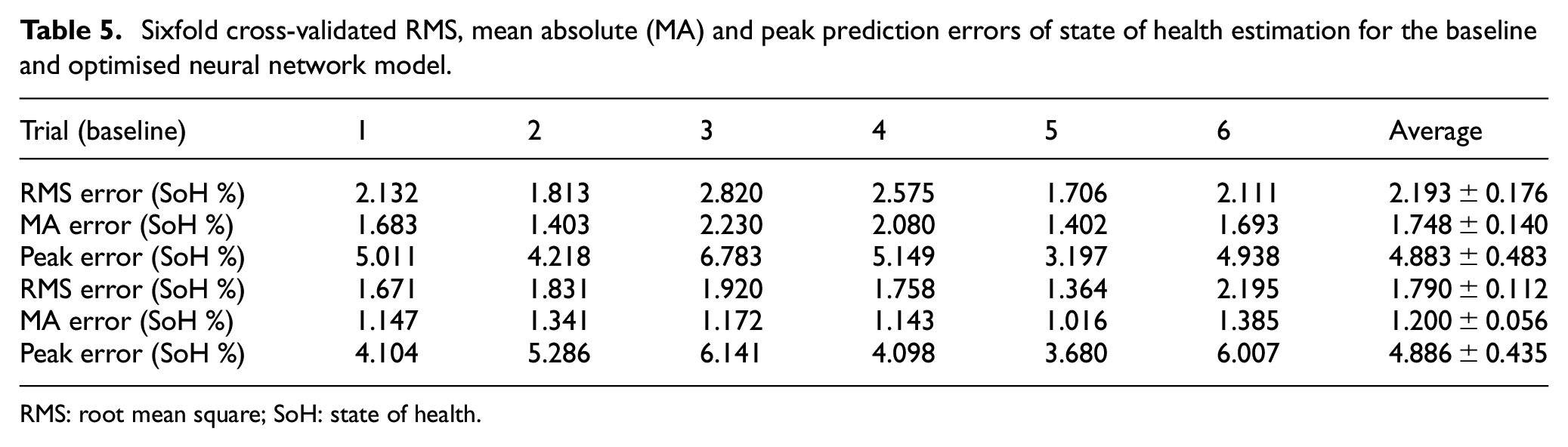
RMS: root mean square; SoH: state of health.
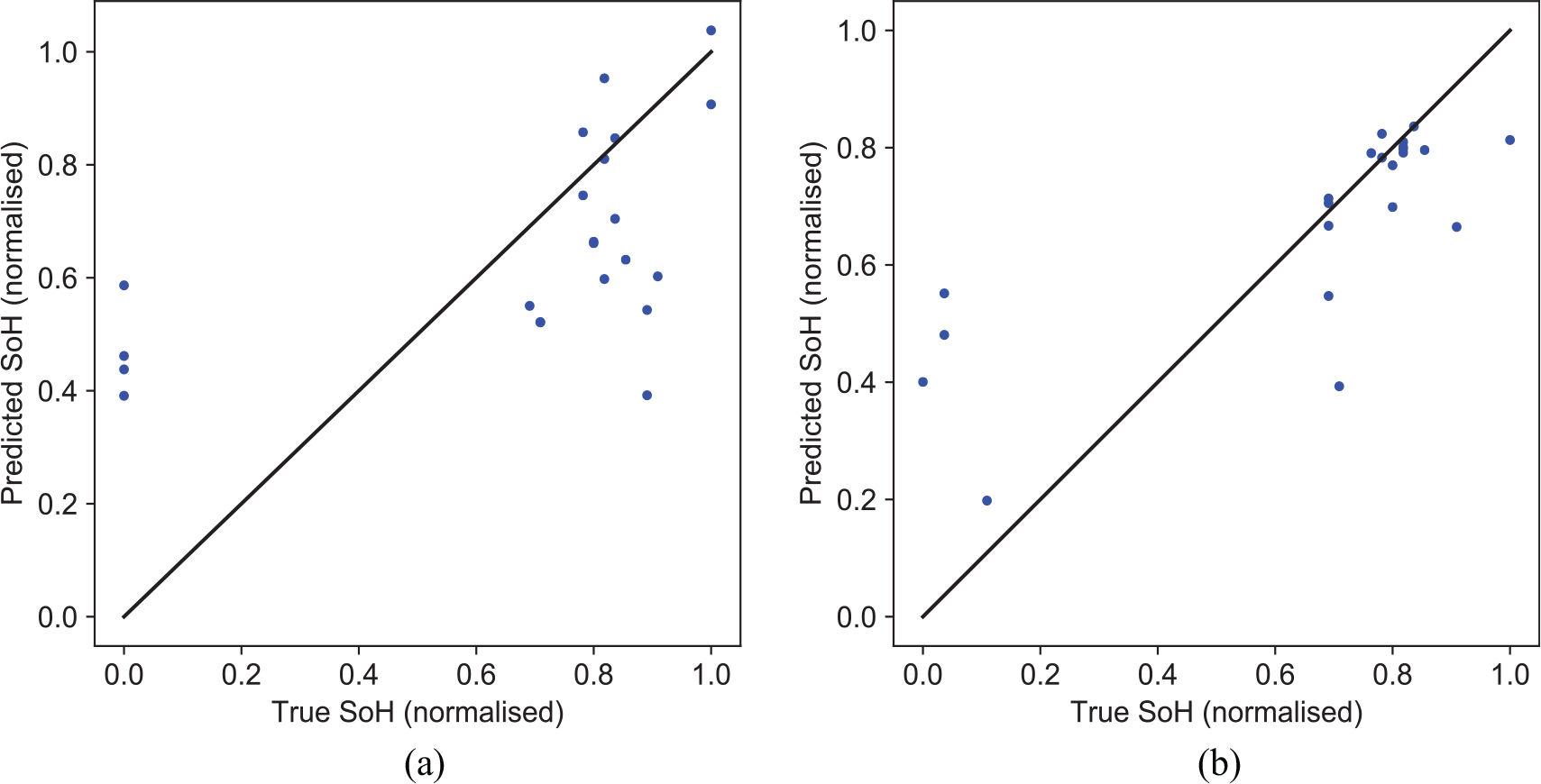
Distribution of predicted versus ground truth state of health values shown as a scatter plot for a single baseline and optimised model cross-validation trial, with RMS errors of 2.314% and 1.679%, respectively: (a) scatter plot for baseline model trial; (b) scatter plot for optimised model trial. The SoH values (range: 77%–85%) are normalised to the range 0–1 for clarity.
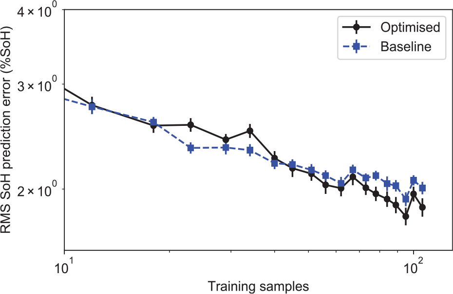
Variation of sixfold cross-validated RMS state of health prediction error for the baseline and hyperparameter optimised model with the number of training samples used.
It is noted that the additional model complexity introduced presents a considerable downside over the baseline model, leading to an increase in training and evaluation times. On the hardware used in this study, the training and evaluation times for the baseline NN were 0.925 ± 0.07 s and 0.023 ± 0.003 s, respectively. For the optimised model, this increases to 6.5 ± 0.7 s and 0.0617 ± 0.0007 s, respectively. In this case, there is mainly a negative impact on training times, with minimal absolute change in evaluation times. Even in the optimised case, the model training times are significantly reduced compared to a convolutional NN-based approach with ensemble learning (143.396 s) 18 of greater complexity; it should also be noted that the quoted time was obtained on considerably more powerful hardware than used in this study. On this basis, the increased level of complexity is therefore deemed acceptable in the scope of this work to improve prediction accuracy.
Optimised network evaluation
The distribution of predictions is an important factor for accurate SoH estimation. It is necessary for both sorting cells given a screening criterion, such as cells being above or below 80% of their original capacity, and for matching of cells of similar SoH that cells are sorted with high accuracy. This necessitates low SoH prediction error and low tendency towards over and under-estimation. Figure 13 presents the model predictions from a trial where the model performed well, achieving an RMS prediction error of 1.570%, and a less well-performing trial with 2.205%. The well-performing trial demonstrates that there is good agreement between the NN predictions and the respective ground truth values, with few outliers and a relatively uniform distribution of predictions in spite of the sparsity of the dataset towards lower SoH values. Results for the less well-performing model suggest that the model generalised well to much of the dataset, however in this case produced a number of outliers. The overall optimised NN performance corresponds to an average RMS prediction error of 1.790% (SoH) over sixfold cross-validation trials as shown in Table 5. In both cases, there is a tendency towards slight over-estimation of SoH towards lower ‘true’ SoH values; however, for the most part, the high and low SoH cells are clearly distinguished from each other.
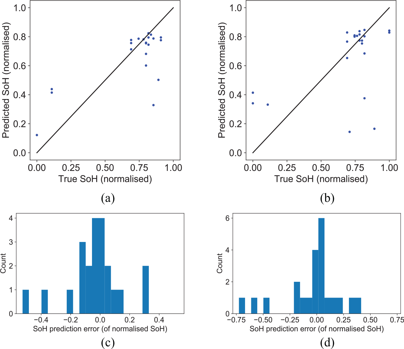
Distribution of predicted versus ground truth state of health values shown as a scatter plot and histogram for high- (RMS error: 1.570%) and low-performing (RMS error: 2.205%) model trials: (a) scatter plot for high-performing trial; (b) scatter plot for low-performing trial; (c) distribution of errors for high-performing trial; and (d) distribution of errors for low-performing trial. The SoH values (range: 77%–85%) are normalised to the range 0–1 for clarity.
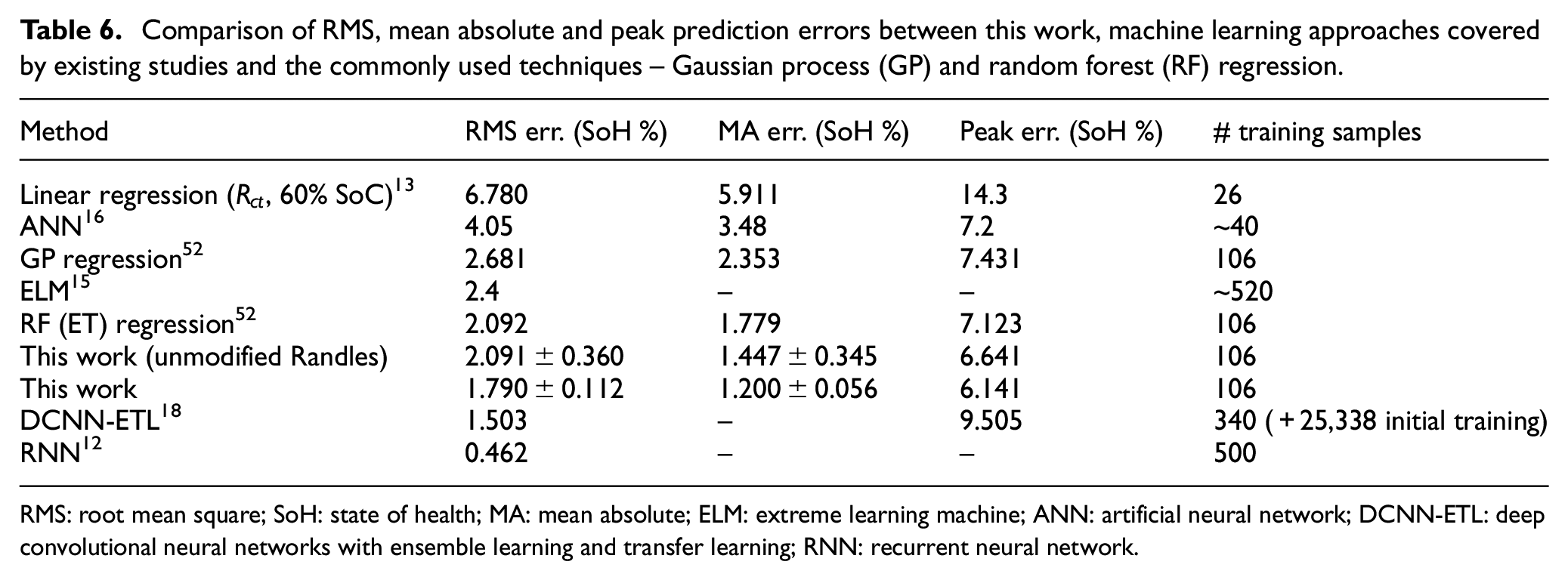
Table 6 summarises the RMS, MA and peak errors of two alternative popular machine learning approaches for small datasets: GP and random forest (RF) ‘extra trees’ regression, using the implementations provided by Pedregosa et al. 52 to estimate SoH using the extracted ECM parameters in comparison with this work. Additionally shown are prediction errors for related SoH estimation schemes presented by previous works.12,13,15,16,18
Comparison of RMS, mean absolute and peak prediction errors between this work, machine learning approaches covered by existing studies and the commonly used techniques – Gaussian process (GP) and random forest (RF) regression.
RMS: root mean square; SoH: state of health; MA: mean absolute; ELM: extreme learning machine; ANN: artificial neural network; DCNN-ETL: deep convolutional neural networks with ensemble learning and transfer learning; RNN: recurrent neural network.
For linear regression, the errors were obtained by application of linear regression of the charge transfer resistance for this work’s dataset as proposed by Wang et al. 13 in this case for data at 60% SoC. For the ELM approach in Densmore and Hanif, 15 the number of training samples is calculated based on the samples available in the open source NASA Ames dataset used. For the ANN approach in Yang et al., 16 the values for RMS error and MA error are calculated from the published test dataset SoH prediction errors, while the number of samples is obtained based on the author quoted value of five cells used for training. The peak error is the maximum quoted error by each of these studies; for this work, it is the maximum error recorded over sixfold cross-validation as shown in Table 5, and provides an indication of the maximum error expected from the SoH estimation method in comparison with related works. As a further comparison, the cross-validation results from the optimised model using the original Randles circuit model introduced in Figure 2 are presented. This ECM describes the impedance data less accurately, increasing the uncertainty in the extracted parameters; this demonstrates how the model predictions are influenced by a suboptimal choice of ECM with additional error on the extracted parameters.
The results of cross-validation trials as shown in Table 6 suggest that a linear regression of the charge transfer resistance is insufficient in this case to accurately predict the battery SoH. The optimised NN model proposed in this work is shown to surpass the performance of well-established regression schemes for the dataset used, while also presenting a reasonable improvement of ∼2.26% over a similar ECM parameter approach 16 for estimating battery SoH, even when considering the smaller dataset used. In this case, the similar performance of the model in this work to that of Yang et al. 16 demonstrates that an ECM approach based on EIS can be directly applied with an ANN model to estimate SoH reliably in spite of the uncertainty introduced by the SoC dependence and the fitting process for the values of extracted ECM parameters. This is corroborated by results for the optimised model presented in this work using the unmodified Randles ECM. Here, there is an increase in 0.301% in the model RMS error compared with the optimised model using the modified Randles circuit, which is most likely caused by the additional fitting error introduced, leading to a less informative set of SoH predictors. However, even in this case, the model still outperforms the original baseline model, RF (ET) and GP regression, even when these approaches are trained with the modified Randles circuit parameters, suggesting the model is able to reduce the influence of fitting error on the overall SoH prediction. Based on the variation of model performance with availability of training data established (Figure 12), it is likely that with a larger dataset of ∼200 samples, the technique proposed reaches parity with the most performant NN approaches such as those by Shen et al. 18
A principal limitation of this work is that the temperature dependence of impedance data has not been considered in this study, and therefore a larger training dataset would be required including temperature as a parameter to make the model robust to temperature changes, or measurements would need to be carried out in a climate-controlled environment. The former could be achieved either by including the temperature directly as a learnable parameter, as with SoC, or normalised to a standard state as proposed by Wang et al. 13 to address this limitation. There is also scope to further reduce the uncertainty inherent in application of non-linear least squares fitting of the raw impedance data imparted to the ECM parameter values obtained. This uncertainty can potentially be reduced by application of a parameter search algorithm, such as those applied by Wang et al. 13 and Tröltzsch et al. 27 Currently, this approach also requires an appropriate choice of ECM based on knowledge of the cell impedance response.
Reduction of measurement times
The primary area of improvement afforded by an ECM parameter–based SoH estimation scheme is additional insight into the battery condition than made available by most SoH monitoring schemes. 6 Another area for potential improvement is improving measurement times associated with collection of impedance data to a level to achieve parity with previous related works such as Bonfitto et al., 17 which operate on 60-s cell I–V profiles to predict SoH. To achieve this, it is possible to target specific frequencies corresponding to regions of interest in an impedance spectrum, such as the double-layer capacitive loop. This particular region of the spectrum in this case lies in the frequency range 1–200 Hz. Such schemes have previously been applied in time critical scenarios such as quality control of fresh batteries, 26 and represent a powerful tool for reduction of measurement times. As a guideline, given a minimum of six probing cycles at each frequency point 26 at six points per decade, it is estimated that measurement times could be reduced to as little as 30 s. To demonstrate this is feasible, fits to the same ECM were performed on the existing dataset using the reduced frequency range as presented in Figure 14, and the optimised model retrained on the extracted parameters.
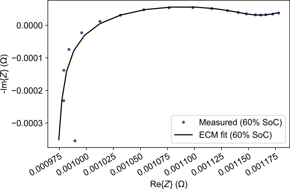
Fit to equivalent circuit model in Figure 4 with experimental impedance data obtained at 60% SoC, 25 °C over the red and white terminals of module 1 of 13, capacity 54.9 A h, limited to the frequency range 1–200 Hz.
The results of further cross-validation trials as summarised in Table 7 suggest that there is potential to greatly improve measurement times with only a small detriment (0.16%) to RMS prediction error. One area of improvement, however, is that the peak prediction error is significantly increased. It is possible that such errors could be reduced by employing ensemble learning techniques as with Shen et al., 18 where the predictions of multiple models were combined to the benefit of accuracy. However, this was considered out of scope for the current work due the constraints of the project to maintain a level of model simplicity, as this further increases the required time to train and evaluate the model.
Sixfold cross-validated RMS, mean absolute and peak prediction errors of state of health estimation for the optimised neural network model using parameters extracted from a reduced frequency range.
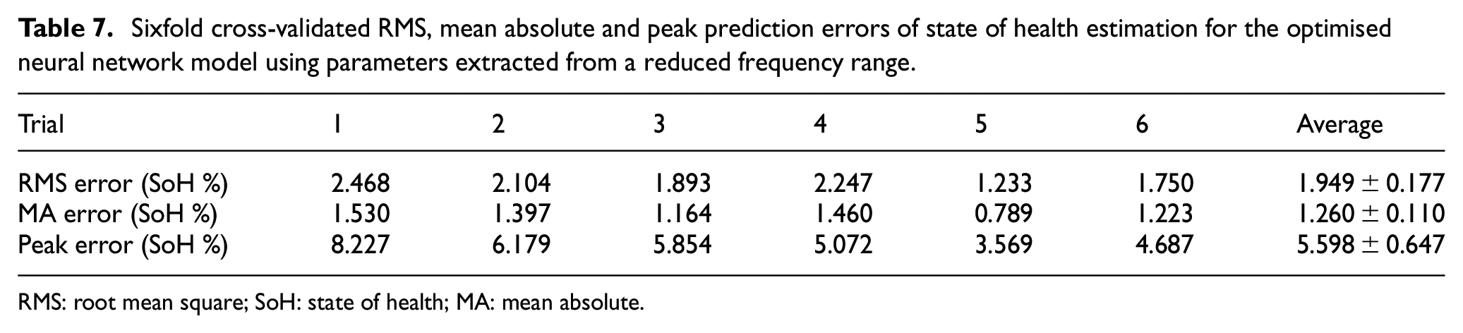
RMS: root mean square; SoH: state of health; MA: mean absolute.
Conclusion
An NN model has been developed to estimate the SoH of 2P arrangements of high-power Lithium Manganese cells based on parameters extracted from impedance spectroscopy data by non-linear least squares fitting to a modified Randles ECM, using a library of impedance and capacity data extracted from 13 Nissan Leaf 2011 battery modules. Starting with a single hidden layer baseline model, an optimised NN was generated by a GP hyperparameter optimisation scheme, which was demonstrated to exceed the performance of the baseline model for training datasets of ∼50 samples. The model cross-validated RMS, MA and peak SoH prediction errors of (1.790 ± 0.112)%, (1.200 ± 0.056)%, and 6.141%, respectively, were demonstrated to be competitive with alternative SoH estimation schemes and exceeds the performance of existing approaches based on extraction of ECM parameters. While the SoC dependence was successfully accounted for by the NN model proposed, a principal limitation of this work is that the temperature dependence of the battery impedance data has not been considered, which ultimately must either be controlled or accounted for by inclusion of temperature as an additional predictor for the SoH or normalisation to a standard state as proposed in previous works. To reduce the measurement times associated with the collection of impedance data, the model performance was assessed based on ECM parameters extracted from a reduced frequency range of 1–200 Hz associated with the capacitive impedance response of the cell. Re-evaluation of the NN model under this condition suggests that there is potential for measurement times to be reduced to as little as 30 s with limited (0.16%) increase in the RMS prediction error, but an increase in the peak prediction error to 8.227%.
Footnotes
Appendix 1
Acknowledgements
The authors would like to thank our partners Dr Musbahu Muhammad, Dr Pierrot Attidekou and the team at Newcastle University for their collaboration and work on the dataset applied in this study.
Data availability statement
The data that support the findings of this study are openly available in Figshare with DOI (10.6084/m9.figshare.12227282). 53
Declaration of conflicting interests
The author(s) declared no potential conflicts of interest with respect to the research, authorship, and/or publication of this article.
Funding
The author(s) disclosed receipt of the following financial support for the research, authorship, and/or publication of this article: This research was conducted as part of the project called ‘Reuse and Recycling of Lithium-Ion Batteries’ (RELIB). This work was supported by the Faraday Institution (grant number: FIRG005).